Distributed Detection with Empirically Observed Statistics
Haiyun He, Lin Zhou, Vincent Y. F. Tan

TL;DR
This paper investigates distributed detection when the underlying distributions are unknown, using noisy empirical statistics, deriving optimal error exponents, and showing that a single channel becomes optimal as training length increases.
Contribution
It introduces a framework for distributed detection with empirically observed statistics and derives the optimal error exponents, extending classical detection results to unknown distributions.
Findings
Optimal type-II error exponent derived for binary detection.
Using one channel is optimal as training length ratio tends to infinity.
Numerical evidence suggests one channel remains optimal for finite training lengths.
Abstract
Consider a distributed detection problem in which the underlying distributions of the observations are unknown; instead of these distributions, noisy versions of empirically observed statistics are available to the fusion center. These empirically observed statistics, together with source (test) sequences, are transmitted through different channels to the fusion center. The fusion center decides which distribution the source sequence is sampled from based on these data. For the binary case, we derive the optimal type-II error exponent given that the type-I error decays exponentially fast. The type-II error exponent is maximized over the proportions of channels for both source and training sequences. We conclude that as the ratio of the lengths of training to test sequences tends to infinity, using only one channel is optimal. By calculating the derived exponents numerically, we…
Click any figure to enlarge with its caption.
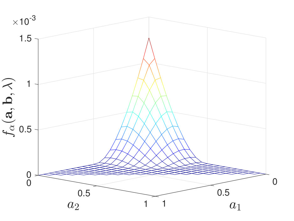 Figure 1
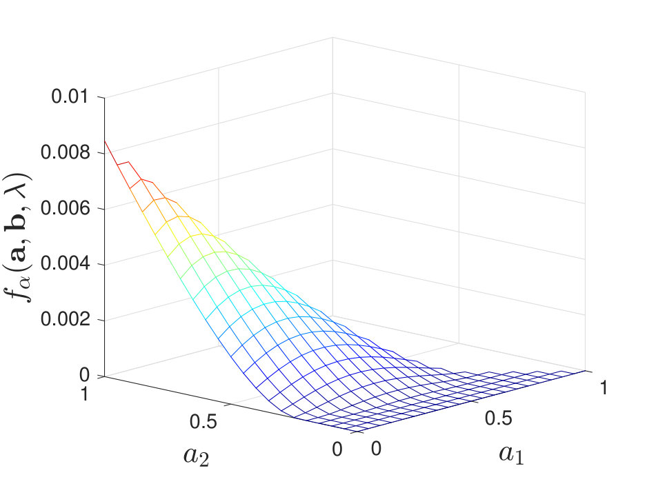 Figure 2
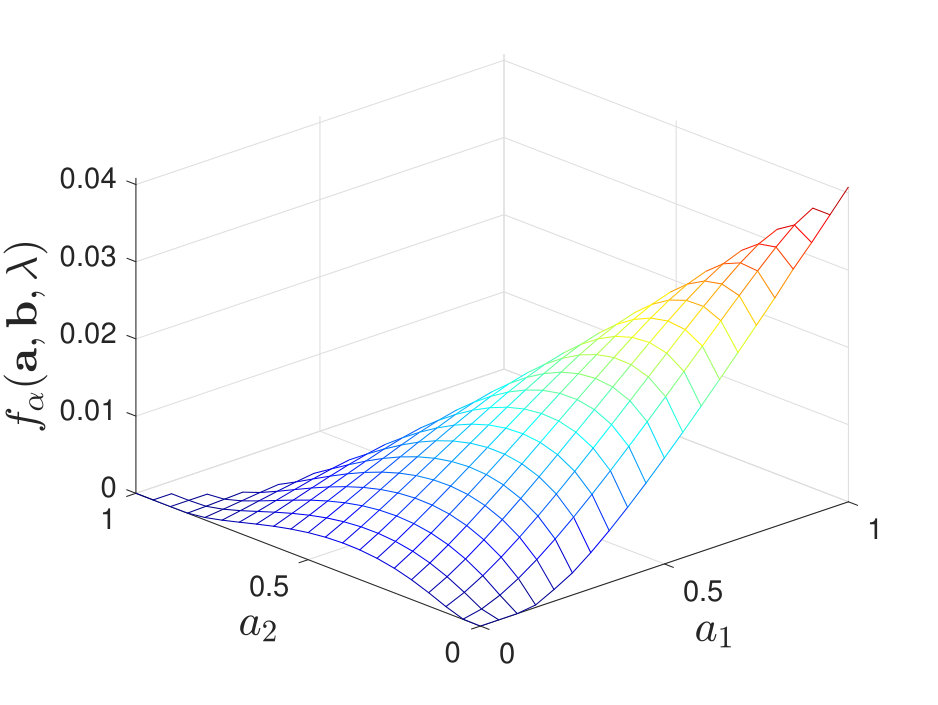 Figure 3
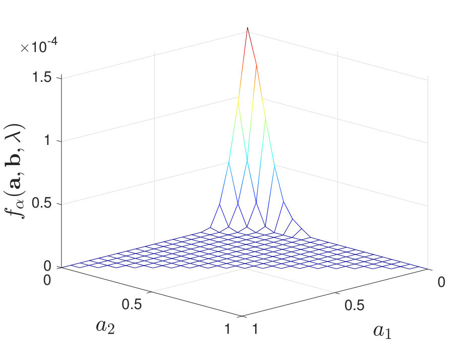 Figure 4
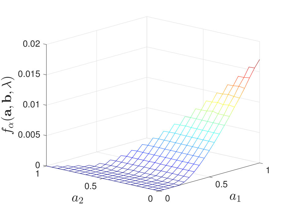 Figure 5
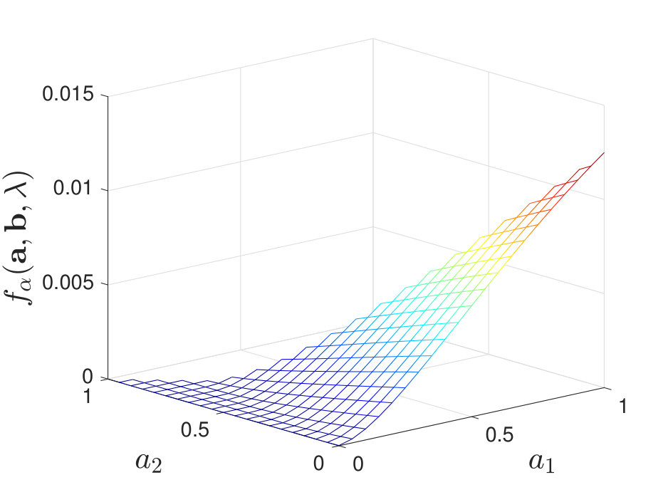 Figure 6
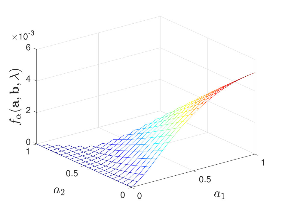 Figure 7
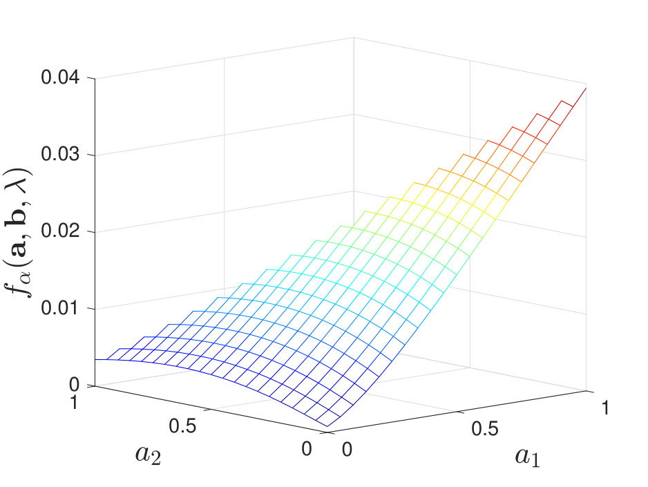 Figure 8
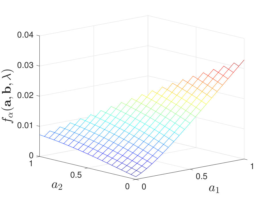 Figure 9
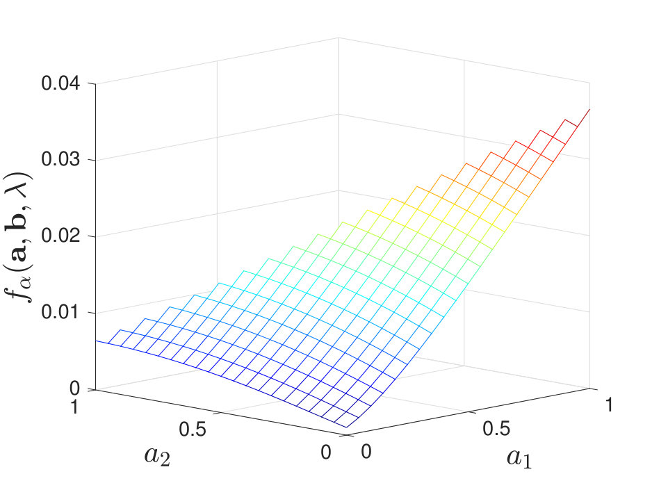 Figure 10
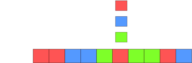 Figure 11
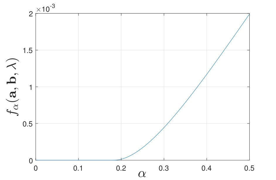 Figure 12
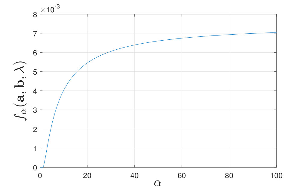 Figure 13
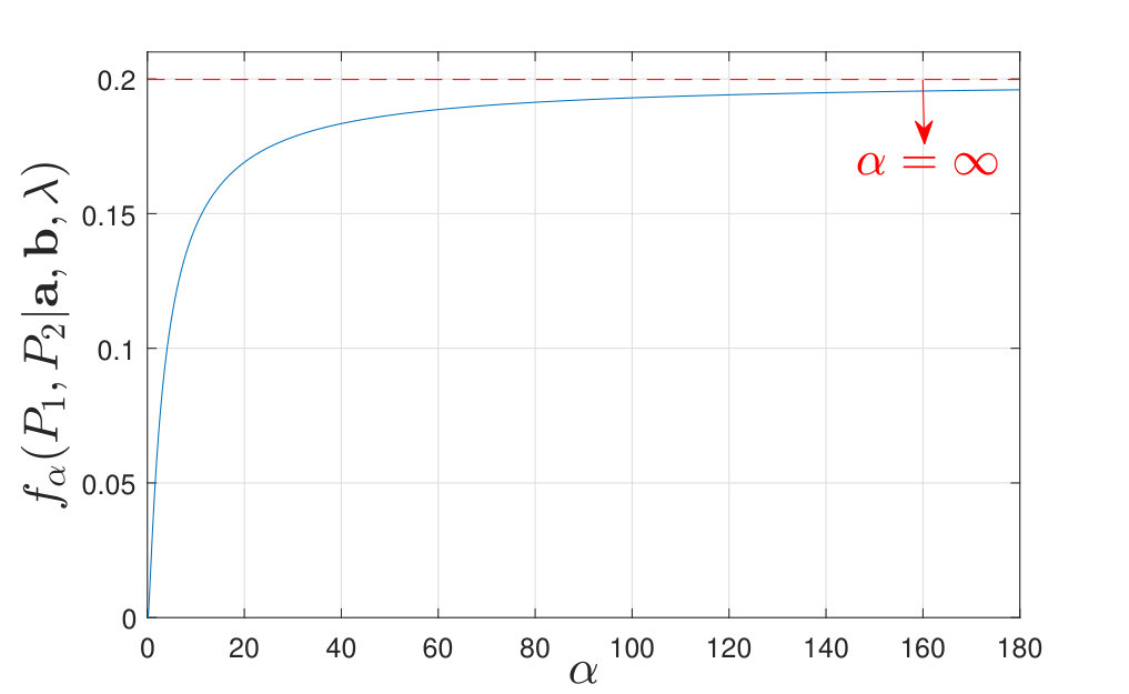 Figure 14
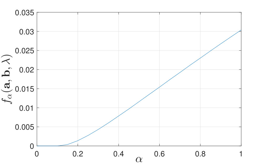 Figure 15
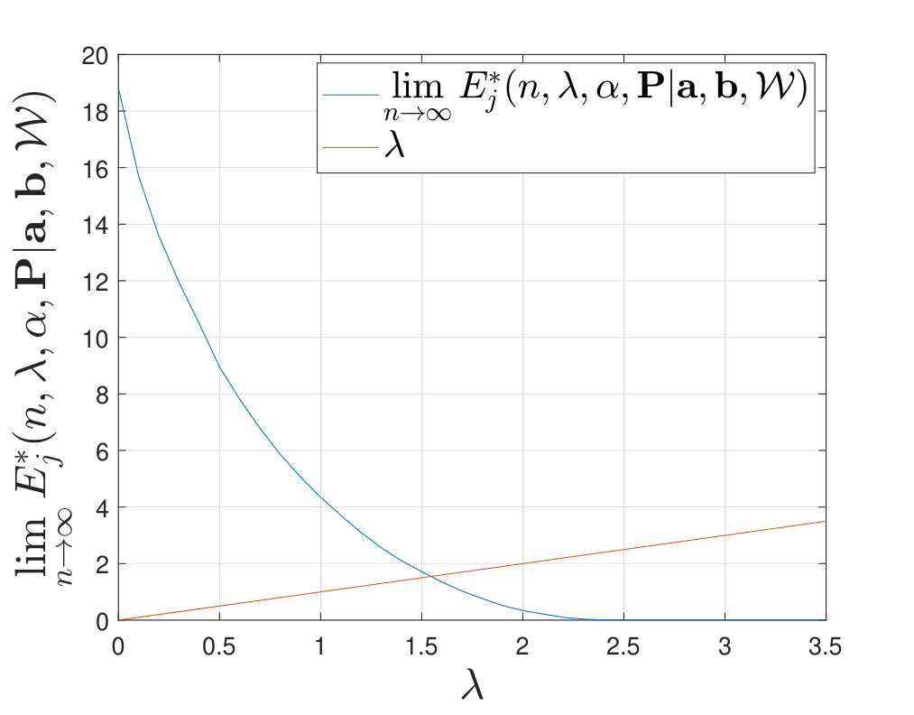 Figure 16
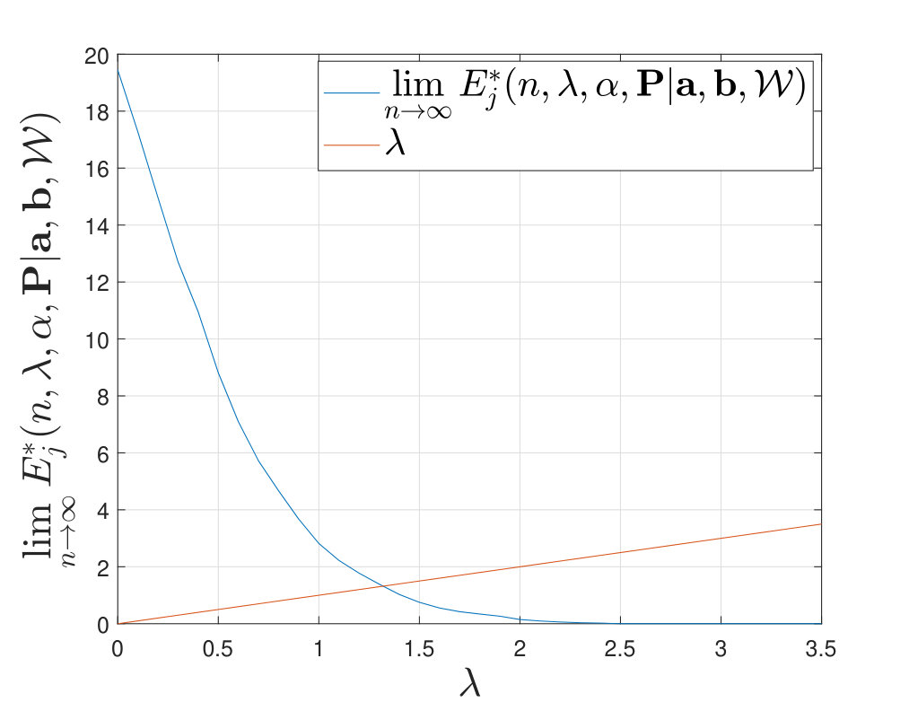 Figure 17
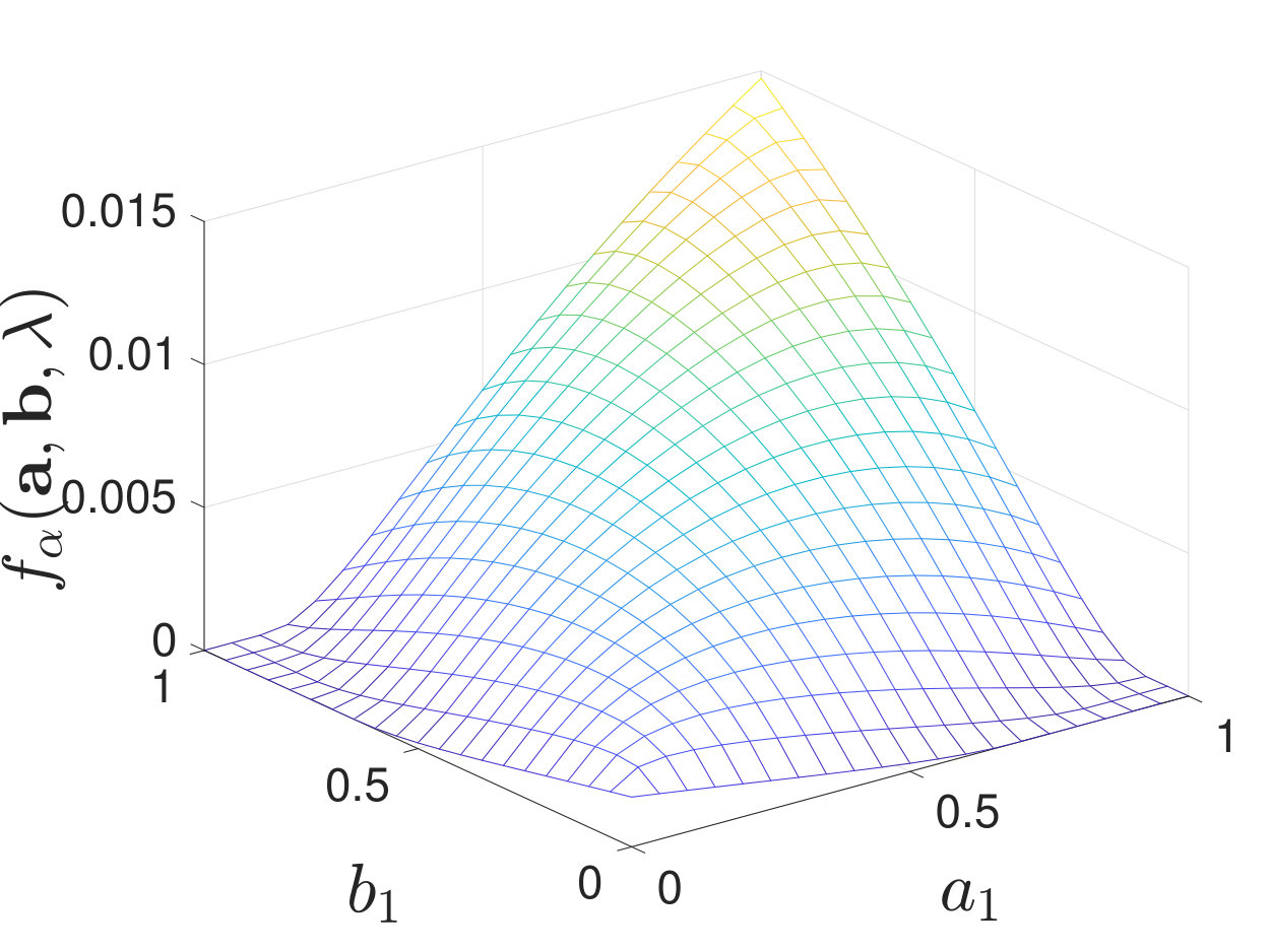 Figure 18
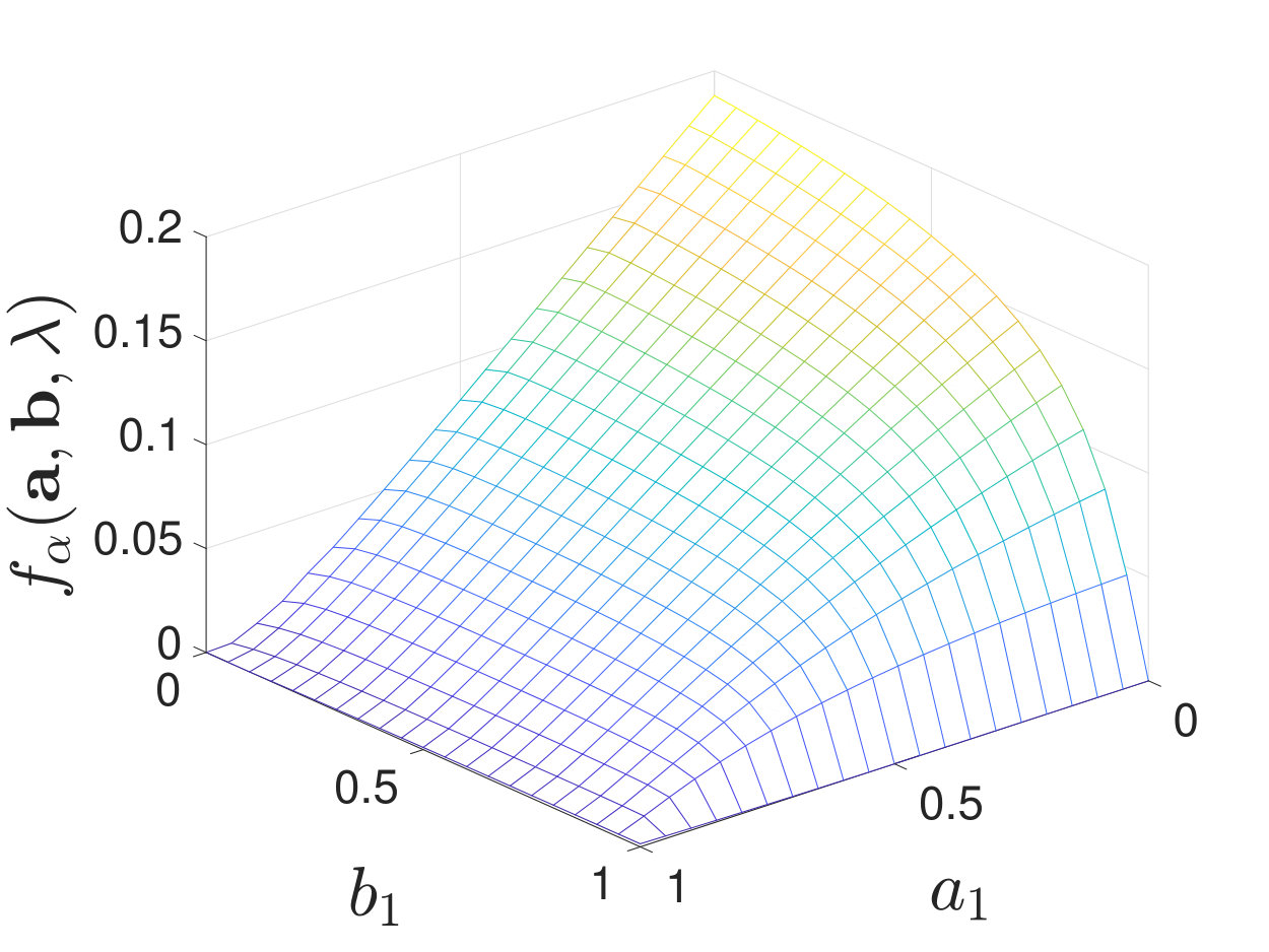 Figure 19
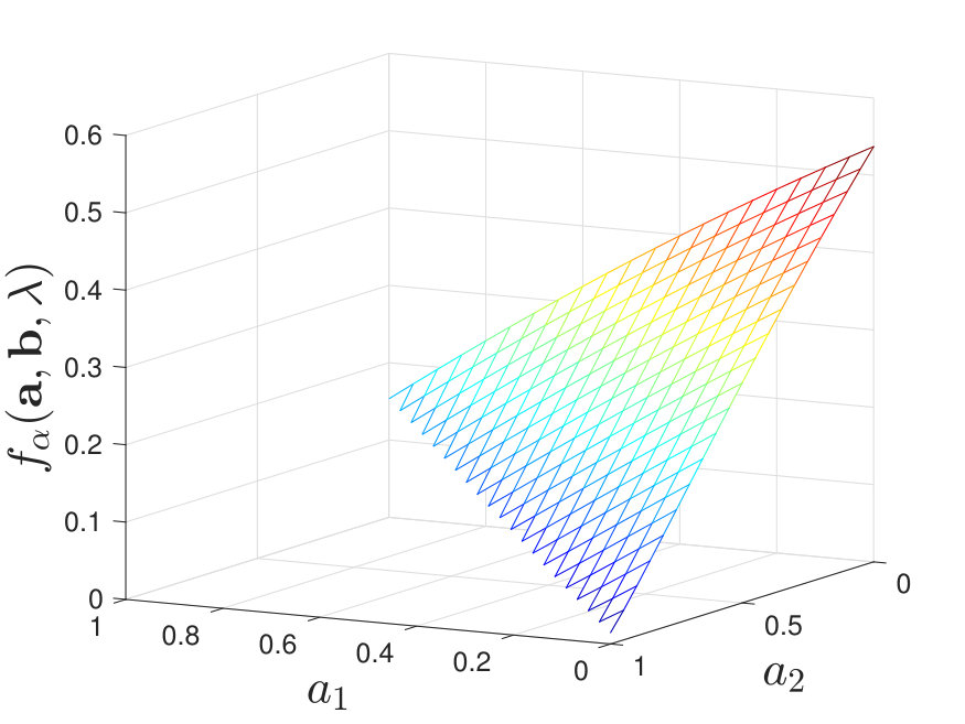 Figure 20
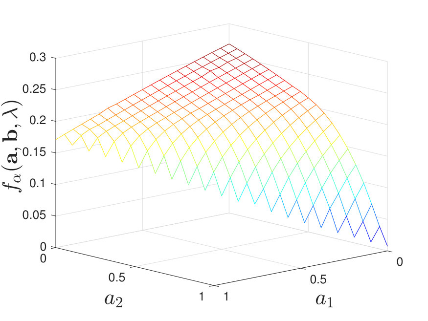 Figure 21
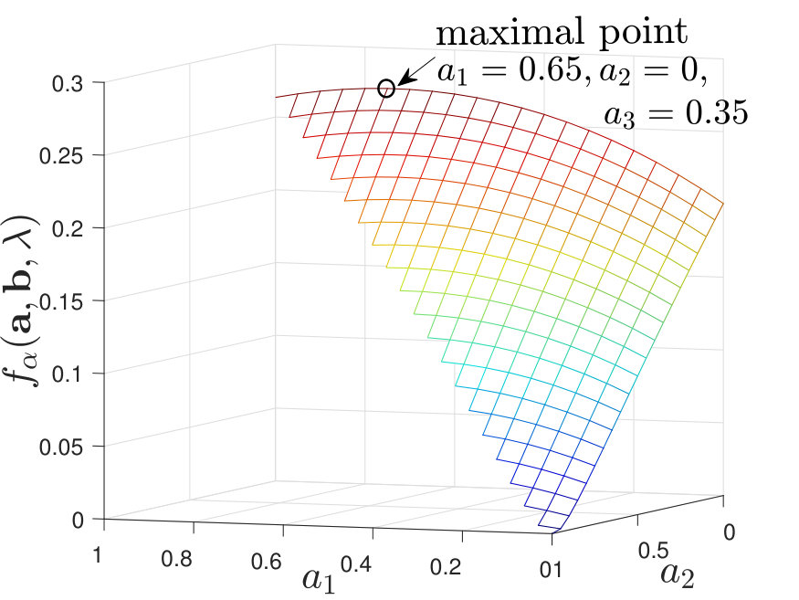 Figure 22
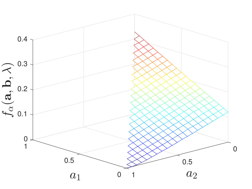 Figure 23
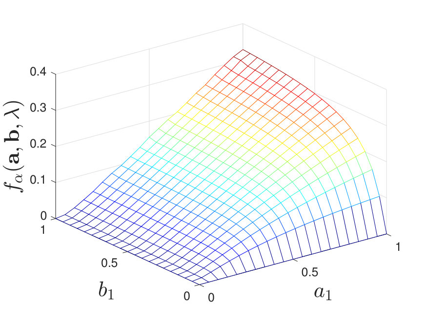 Figure 24
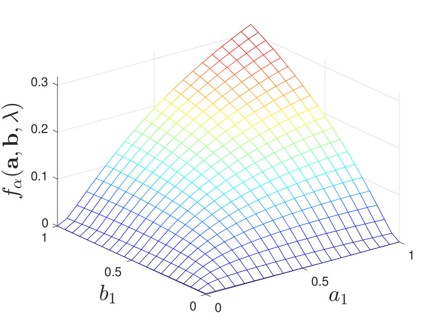 Figure 25
Peer Reviews
No public reviews on file for this paper yet. If you reviewed it on a platform where reviews are public (OpenReview, ICLR, NeurIPS, ICML), you can paste yours below so the community can read it here.
Videos
No videos yet. Explain this paper in a talk, walkthrough, or lecture? Add one.
Distributed Detection with
Empirically Observed Statistics
Haiyun He, Student Member, IEEE Lin Zhou, *Member, IEEE * Vincent Y. F. Tan, Senior Member, IEEE This work is funded by a Singapore National Research Foundation Fellowship (R-263-000-D02-281) and the Research Scholar Budget (RSB) from NUS (C-261-000-207-532 and C-261-000-005-001).This paper was presented in part at the IEEE Information Theory Workshop in Visby, Gotland, Sweden, 2019.H. He and V. Y. F. Tan are with the Department of Electrical and Computer Engineering, National University of Singapore (NUS) (Emails: [email protected] and [email protected]). V. Y. F. Tan is also with the Department of Mathematics, NUS. L. Zhou is with the Department of Electrical Engineering and Computer Science, University of Michigan, Ann Arbor (Email: [email protected]).Copyright (c) 2017 IEEE. Personal use of this material is permitted. However, permission to use this material for any other purposes must be obtained from the IEEE by sending a request to [email protected].
Abstract
Consider a distributed detection problem in which the underlying distributions of the observations are unknown; instead of these distributions, noisy versions of empirically observed statistics are available to the fusion center. These empirically observed statistics, together with source (test) sequences, are transmitted through different channels to the fusion center. The fusion center decides which distribution the source sequence is sampled from based on these data. For the binary case, we derive the optimal type-II error exponent given that the type-I error decays exponentially fast. The type-II error exponent is maximized over the proportions of channels for both source and training sequences. We conclude that as the ratio of the lengths of training to test sequences tends to infinity, using only one channel is optimal. By calculating the derived exponents numerically, we conjecture that the same is true when is finite under certain conditions. We relate our results to the classical distributed detection problem studied by Tsitsiklis, in which the underlying distributions are known. Finally, our results are extended to the case of -ary distributed detection with a rejection option.
Index Terms:
Distributed detection, Error exponents, Training samples, Hypothesis testing
I Introduction
The problem of distributed detection [1, 2] has a plethora of applications, such as in distributed radar and sensor networks; see [3] and references therein for an overview. In these examples, the observed information at local sensors (processors) needs to be quantized before being sent to a fusion center. The fusion center then performs a specific inference task such as hypothesis testing.
In the traditional distributed detection problem as studied in [1, 2, 3, 4], the underlying generating distributions are available at the fusion center and one is tasked to design a test based on observations as well as the known distributions. However, in practical applications, the fusion center has no knowledge of the underlying distributions and may only be given quantized or noisy observations and labelled training sequences (in place of the generating distributions). This leads to new challenges in designing optimal tests.
Motivated by these practical issues and inspired by [5, 2], in this paper, we adopt a contemporary statistical learning approach and consider the distributed detection problem as shown, for the binary case, in Figure 1 in which the distributions of sensor observations are unknown. We term this problem as distributed detection with empirically observed statistics. We assume that the sensor observations are transmitted to the fusion center via different channels, which can also be regarded as compressors. Labelled training sequences generated from the different underlying distributions are pre-processed then provided to the fusion center. Our aim is to derive fundamental performance limits of the classification problem as well as to potentially come up with the same conclusions as Tsitsiklis did in [2], i.e., to conclude that a small number of distinct channels or local decision rules suffices to attain the optimal error exponent.
I-A Main Contributions
In this paper, our main contributions are as follows.
Firstly, for the binary distributed detection problem, we derive the asymptotically optimal type-II error exponent when the type-I error exponent is lower bounded by a positive constant. In the achievability proof, we introduce a generalized version of Gutman’s test in [5] and prove that the so-designed test is asymptotically optimal.
Secondly, again restricting ourselves to the binary case, we discuss the optimal proportions of different channels that serve as pre-processors of the training and source sequences. Let , a constant, denote the ratio between the length of the training sequence and the length of the source sequence. When , we provide a closed-form expression for the type-II error exponent and prove that using only one identical channel for both training and source sequences is asymptotically optimal. This mirrors Tsitsiklis’ result [2]. On the other hand, if is sufficiently small, the type-II error exponent is identically equal to zero. When does not take extreme values, by calculating the derived exponent numerically, we conjecture that using one channel for the training sequence and another (possibly the same one) for the source sequence is optimal under certain conditions.
Thirdly, we relate our results to the classical distributed detection problem in Tsitsiklis’ paper [2]. When , the true distributions can be estimated to arbitrary accuracy and we naturally recover the results in [2] for both the Neyman-Pearson and Bayesian settings.
Finally, we extend our analyses to consider an -ary distributed detection problem with rejection. We derive the asymptotically optimal type- rejection exponent for each under the condition that all (undetected) error exponents are lower bounded by a positive constant . In the achievability proof, we introduce a generalized version of Unnikrishnan’s test [6] by identifying an appropriate test statistic.
I-B Related Works
The distributed detection literature is vast and so it would be futile to review all existing works. This paper, however, is mainly inspired by [5] and [2]. In [5], Gutman proposed an asymptotically optimal type-based test for the binary classification problem. In [2], Tsitsiklis showed that using distinct local decision rules is optimal for -ary hypotheses testing in standard Bayesian and Neyman-Pearson distributed detection settings. Ziv [7] proposed a discriminant function related to universal data compression in the binary classification problem with empirically observed statistics. Chamberland and Veeravalli [8] considered the classical distributed detection in a sensor network with a multiple access channel, capacity constraint and additive noise. Liu and Sayeed [9] extended the type-based distributed detection to wireless networks. Chen and Wang [10] studied the anonymous heterogeneous distributed detection problem and quantified the price of anonymity. Tay, Tsitsiklis and Win studied tree-based variations of the distributed detection problem in the Bayesian [4] and Neyman-Pearson settings [11]. The authors also studied Bayesian distributed detection in a tandem sensor network[12]. The aforementioned works assume that the distributions are known.
Nguyen, Wainwright and Jordan[13] proposed a kernel-based algorithm for the nonparametric distributed detection problem with communication constraints. Similarly, Sun and Tay[14] also studied nonparametric distributed detection networks using kernel methods and in the presence of privacy constraints. While the problem settings in [13] and [14] involve training samples, the questions posed there are algorithmic in nature and hence, different. In particular, they do not involve fundamental limits in the spirit of this paper.
I-C Paper Outline
The rest of this paper is organized as follows. In Section II, we formulate the distributed detection problem with empirically observed statistics. We also present the optimal type-II error exponent and analyze the optimal proportion of channels and recover analogues of the results in [2] both for Neyman-Pearson and Bayesian settings. In Section III, we extend our results to the case in which there are hypotheses and the rejection option is present. We conclude our discussion and present avenues for future work in Section IV. The proofs of our results are provided in the appendices.
I-D Notation
Random variables and their realizations are in upper (e.g., ) and lower case (e.g., ) respectively. All sets are denoted in calligraphic font (e.g., ). We use to denote the complement of . Let be a random vector of length . All logarithms are base . Given any two integers , we use to denote the set of integers and use to denote . The set of all probability distributions on a finite set is denoted as and the set of all conditional probability distributions from to is denoted as . Given and , we use to denote the marginal distribution on induced by and . We denote the support of as . Given a vector , the type or empirical distribution [15] is denoted as where . We interchangeably use and to denote the type class of . Let denote the set of types with denominator . For two positive sequences and , we write if . The notations and are defined similarly. For a given vector , we let denote the support of .
II Binary Distributed Detection with Training Samples
In this section, we formulate the problem in which there are two hypotheses and instead of distributions, only training samples are available.
II-A Problem Formulation
We assume that there are fixed compressors or channels (these are called local decision rules in [2]), where for each , the -th channel is . This channel has input alphabet and output alphabet . For notational simplicity, we assume that but our results go through for uncountably infinite as well. We let be a fixed set of channels. Furthermore, let and to be functions that map the index of the test/training sample to the channel index.
The system model is as follows (see Figure 1). There are sensors and a source/test sequence generated i.i.d. according to some unknown distribution defined on . For each , the -th sensor observes and maps it to using the channel . The ’s from all local sensors are transmitted to a fusion center. In addition to ’s, the fusion center observes two noisy versions of training sequences which are generated i.i.d. according to some unknown but fixed distributions . The fusion center observes noisy sequences , where and for all . With and , the fusion center uses a decision rule to discriminate between the following two hypotheses:
- •
: the source sequence and the training sequence are generated according to the same distribution;
- •
: the source sequence and the training sequence are generated according to the same distribution.
We assume for some .111We ignore the integer constraints of and write . For each , we use and to denote the proportions of and in which the channel is used to process the source and training sequences respectively, i.e.,
[TABLE]
An example is given in Figure 2. Furthermore, we let and . We assume that the following limits exist:
[TABLE]
To avoid clutter in subsequent mathematical expressions, we abuse notation subsequently and drop the superscript in and in all non-asymptotic expressions, with the understanding that (resp. ) appearing in a non-asymptotic expression should be interpreted as (resp. ).
Given any decision rule at the fusion center and any pair of distributions according to which the training sequences are generated, the performance metrics we consider are the type-I and type-II error probabilities
[TABLE]
where for , we use to denote the joint distribution of and under hypothesis . In the remainder of this paper, we use to denote if there is no risk of confusion.
Inspired by [5], in this paper, we are interested in the maximal type-II error exponent with respect to a pair of target distributions for any decision rule at the fusion center whose type-I error probability decays exponentially fast with a certain fixed exponential rate for all pairs of distributions, i.e., given any , the optimal non-asymptotic type-II error exponent is
[TABLE]
II-B Definitions
To state our results succinctly, we begin by stating some somewhat non-standard definitions. Given any pair of distributions and any , the generalized Jensen-Shannon divergence [16, Eqn. (3)] is defined as
[TABLE]
Let and where be three collections of distributions. Given any , any , any , any pair , define the following linear combination of divergences
[TABLE]
and furthermore, given any , define the following set of collections of distributions
[TABLE]
Finally, define the following minimum linear combination of divergences over the collections of distributions in as
[TABLE]
II-C Main Results
The following theorem is our main result and presents a single-letter expression for the optimal type-II exponent.
Theorem 1**.**
Given any , any pair of target distributions ,
[TABLE]
The proof of Theorem 1 is given in Appendix -A. Several remarks are in order.
Firstly, in the achievability proof of Theorem 1, we make use of the following test at the fusion center
[TABLE]
where we suppressed the dependence of on and for each , we use to denote the collection of where satisfies and similarly for for . Furthermore, we use to denote the vector of types and use for similarly. Theorem 1 indicates that the test in (II-C) is asymptotically optimal. The test in (II-C) basically compares a certain distance between and plus a bias term related to to a threshold . When the distance is small enough, we declare that and are generated according to the same distribution; otherwise, we declare that they are not.
Secondly, the test in (II-C) is a generalization of Gutman’s test in [5]. To see this, we note that if we let , and consider the deterministic channel denoted as , the test in (II-C) reduces to Gutman’s test using since
[TABLE]
and the exponent in Theorem 1 reduces to the type-II exponent for binary classification [5, Thm. 3], i.e.,
[TABLE]
and
[TABLE]
Finally, to better understand the effect of not knowing the true distributions, we numerically plot the optimal type-II exponent (defined in (8)) in Figure 3. As shown in Figure 3, the optimal type-II exponent increases as increases and converges to a threshold as . This threshold is the optimal error exponent when the true distributions are known [2, Theorem 2]. The gap thus quantifies the loss due to the fact that the generating distributions are unknown and only training samples are available to the learner.
II-D Further Discussions on the Impact of the Proportions of Local Decision Rules on the Exponent
In this subsection, we discuss the choices of the proportion of local decision rules, denoted by , to achieve the optimal type-II exponent . Throughout the section, we fix a pair of target distributions . For brevity, we define
[TABLE]
Since the type-II error exponent depends on , inspired by the result in [2] which states that one local decision rule is optimal for binary hypotheses testing (in the Neyman-Pearson and Bayesian settings), we can further optimize the type-II error exponent with respect to the design of the proportion of channels (encoded in and ) and thus study
[TABLE]
and the corresponding optimizers and for different values of . For this purpose, given any vector and any distribution , define
[TABLE]
Note that and if , then for all .
Furthermore, given any , any and any pair , let
[TABLE]
Lemma 2**.**
The function satisfies
[TABLE]
The proof of Lemma 2 is provided in Appendix -B.
We say that is deterministic if there exists a such that . Let be the -th standard basis vector in , i.e., the vector equals in the -th location and [math] in other locations.
Corollary 3**.**
*Given any , we have *
[TABLE]
and thus the maximizers for satisfy that are both deterministic and .
The proof of Corollary 3 is provided in Appendix -C. Corollary 3 says that when the length of the training sequence is much longer than the test sequence, it is optimal to use a single local decision rule or channel to pre-process the training data and source sequence; this is analogous to [2, Theorem 1].
Given any and any , let
[TABLE]
Given any , let be the solution (in ) to the following equation
[TABLE]
Since is an increasing function of and , for any , we have unless .
Lemma 4**.**
Given any and any , if , then
[TABLE]
We verified Lemma 4 numerically by plotting as a function of when is small for certain values of in Figure 4. The proof of Lemma 4 is straightforward since when , where , and and thus . The intuition is that when is small enough, for any , the decision rule in (II-C) always declares , which means that , so the corresponding exponent is identically [math].
II-E * Numerical Study on Optimal Proportions of Local Decision Rules*
In the following, we present numerical results to illustrate the properties of the optimal proportions of local decision rules when ; that is, is moderate.
When , regardless of the stochasticity of the channels in , we find that the maximal value of always lies at a corner point of the feasible set of . See Figure 5 for numerical examples. When , we find that the results are more involved and it is not necessarily optimal to use only one local decision rule. To clarify our observations, we first describe cases where our numerical calculations of the exponent suggest that it is optimal to use only one local decision rule to achieve the optimal type-II error exponent; this is analogous to [2, Theorem 2]. We then consider other cases and briefly discuss why it is not always optimal to use one local decision rule.
II-E1 When One Local Decision Rule is Optimal
In most practical distributed detection systems, the local decision rule at each sensor is a deterministic compressor or quantizer. However, under certain conditions, randomized local decision rules can be used to provide privacy [17, 18, 19] or to satisfy power constraints [20, Sec. IV]. We now describe a class of local decision rules for which the exponent can be simplified and numerical calculations of the exponents suggest that full diversity of local decision rules is unnecessary.
Let be the set of stochastic matrices (channels) with rows and columns whose rows contain a permutation of the rows of , the identity matrix. The set includes all deterministic mappings (e.g., Figure 6(b)) and a subset of stochastic mappings as long as for each , there exists an that maps directly to it, as illustrated in Figure 6(a). Note that Tsitsiklis [2] considers only deterministic local decision rules, which certainly falls into the class . The definition is extended in the obvious way if (i.e., for all , there exists such that ).
We assume that the second training sequence is pre-processed by one local decision rule , i.e., for all . The channels that are used to pre-process the test sequence and the first training sequence are arbitrary. Under such a setting, we can simplify the asymptotically optimal error exponent and test (cf. (9) and (II-C)) as follows:
[TABLE]
where \mathcal{Q}_{\lambda,{\mathcal{V}_{\mathrm{I}}}}(\alpha,\mathbf{a},\mathbf{b},\mathcal{W}):=\big{\{}(\mathbf{Q},\tilde{\mathbf{Q}})\in\mathcal{P}([L])^{K}:\min_{\tilde{P}\in\mathcal{P}(\mathcal{X})}\sum_{k\in[K]}\big{(}a_{k}D(Q_{k}\|\tilde{P}W_{k})+\alpha b_{k}D(\tilde{Q}_{k}\|\tilde{P}W_{k})\big{)}\leq\lambda\big{\}}, and is given in (30) at the top of the next page.
By calculating for various and , we find that when is moderate (i.e., neither nor ), the maximal value of always lies at a corner point of the feasible set of , as shown in Figure 7. Additional numerical results are shown in Appendix -D. Inspired by these numerical results, we present the following conjecture:
Conjecture 5**.**
For all , the vectors and that maximize are deterministic if the second training sequence is pre-processed by a single channel .
II-E2 Results without Assumptions on Channels
In this subsection, we discuss the general case where there is no assumption (e.g., deterministic or membership in ) on local decision rules used to pre-process , and .
By calculating for various and , we find that when and is moderate, the maximal value of does not always lie at a corner point; instead, it may occur at non-corner points within the feasible set of . We illustrate this in Figure 8 for the case of stochastic and for some .
Our numerical results suggest that without the knowledge of true distributions, it is not always optimal to use only one identical channel to process the test and training samples, which differs from the result in Tsitsiklis’ paper [2]. The difference can be explained intuitively as follows. First, in [2], deterministic decision rules are considered while in our setting, we allow the channels to be stochastic. Second, when is moderate, we are not able to estimate the true distributions with arbitrary accuracy using the training samples. Thus, to combat the randomness induced by the channels and to compensate for the loss of (full) knowledge of the true distributions, the fusion center may require more information; hence the need for more diversity in the local decision rules.
II-F Connections to Results in Distributed Detection
We discuss the connections between Theorem 1 and [2], which concerns distributed detection when the underlying distributions are known. Throughout this subsection, to emphasize the dependence of error probabilities on , we use to denote the type- error probability with respect to distributions when test is used at the fusion center.
We first consider the Neyman-Pearson setting [21, Sec. 11.8]. Given any , let be the set of tests satisfying that for all ,
[TABLE]
Let the optimal type-II error probability subject to (31) be
[TABLE]
Note that depends on , and but this dependence is suppressed for the sake of brevity.
Corollary 6**.**
Given any and any ,
[TABLE]
Proof sketch of Corollary 6.
The direct parts of the result are corollaries of Theorem 1, Lemma 2 and Corollary 3 by letting . The converse parts follow from [2, Theorem 2] where the distributions are known since one can never obtain better (larger) exponents with unknown distributions than with known distributions. Since the justifications are straightforward, we omit the details for the sake of brevity. ∎
We also consider the Bayesian setting. Assume the prior probabilities for and are and respectively. Clearly, . Given any and any , let the Bayesian error probability be
[TABLE]
Furthermore, let the maximum Chernoff information between and be
[TABLE]
and let be the set of tests at the fusion center satisfying that for all ,
[TABLE]
Finally, let the optimal Bayesian error probability be
[TABLE]
Again depends on both and .
Corollary 7**.**
Given any and any ,
[TABLE]
Proof sketch of Corollary 7.
The direct parts of the following results are corollaries of Theorem 1, Lemma 2 and Corollary 3 by solving . The (strong) converse parts follow from [2]. ∎
Under the Bayesian setting, the exponents of the type-I and type-II error probabilities are equal [21, Thm. 11.9.1].
Note that Corollaries 6 and 7 are analogous to distributed detection [2] for the binary case under the Neyman-Pearson and Bayesian settings respectively where the true distributions are known. The intuition is that when the lengths of the training sequences are much longer than that of the source sequence (i.e., ), we can estimate the true distributions to arbitrary precision, i.e., as accurately as desired.
III -ary Distributed Detection with the Rejection Option and Training Samples
In this section, we generalize the binary distributed detection problem to the scenario in which we desire to discriminate between hypotheses with the rejection option. Our main contribution here is the identification of an appropriate test statistic and test that achieves the optimal rejection exponent for a fixed lower bound on all error exponents.
III-A Problem Formulation
In the -ary distributed detection problem, there are training sequences , each generated i.i.d. according to an unknown distribution . There are sensors. Each sensor observes a source symbol and compress/processes it into a noisy version just as in the binary distributed detection problem. Given noisy training sequences and the compressed source sequence , in which for all and , the fusion center uses a decision rule to discriminate among the following hypotheses:
- •
: the source sequence and the -th training sequence are generated according to the same distribution;
- •
: the source sequence is generated according to a distribution different from those which the training sequences are generated from and hence we reject all .
Thus, the decision rule partitions the sample space into disjoint regions: acceptance regions , where favors hypothesis , i.e.,
[TABLE]
and one rejection region which favors hypothesis . Note that here we assume that all training sequences are processed with channels in using the same index mapping function . That is, all the first components are passed through the same channel, which is one element from . The same is true for all the other components.
For conciseness, we set and use similarly. Furthermore, we set and use and similarly. Recall the definition of and the assumption that . Given any decision rule at the fusion center and any tuple of distributions , the performance metrics we consider are the error probabilities and the rejection probabilities for each , i.e.,
[TABLE]
We use and in place of and respectively if there is no risk of confusion. For this setting, we are interested in tests that can simultaneously ensure exponential decay of the error probabilities under any hypothesis for any tuple of distributions and exponential decay of the rejection probabilities under each hypothesis for a particular tuple of distributions. To be concrete, given any tuple of distributions and any , we are interested in the following optimal exponent of the rejection probability under hypothesis :
[TABLE]
We emphasize that in this formulation, under each hypothesis, the error exponent is at least for all tuples of distributions.
III-B Main Results
Before presenting the main result, we present some preliminary definitions. Recall that for each , we use to denote the collection of satisfying , use to denote and use to denote the vector of types . Similarly, for each and , we use the notations , and . Given any tuple of distributions and any , define the following linear combination of divergences
[TABLE]
and furthermore, let
[TABLE]
Note that is a slight generalization of in (6).
In the following, we will see that is an appropriate test statistic that will be used in the achievability proof and an optimized version of is the corresponding exponent. Finally, given any satisfying , we define the following set of the collections of distributions:
[TABLE]
Note that if we choose such that and for any , then for all , we have
[TABLE]
and
[TABLE]
which implies that for all . Thus, is non-empty for any .
Our main result in this section is the following asymptotic characterization of .
Theorem 8**.**
Given any and any tuple of target distributions , for all , we have
[TABLE]
The proof of Theorem 8 is given in Appendix -E.
First, as shown in Fig. 9, there exists such that , which implies that the type- rejection exponents can be designed to be smaller than all the error exponents with an appropriate choice of . This scenario is reminiscent of practical communication scenarios [22, 23] (automatic repeat request or ARQ) where the rejection probability is designed to be much larger than the (undetected) error probability as declaring a rejection is typically much less costly than a genuine mistake being made.
Second, let us describe the test that is used in the achievability proof of Theorem 8. This test is a generalized version of Unnikrishnan’s test [6]. Given any tuple of types , we define the indices of the minimum and the second minimum of over all as
[TABLE]
and
[TABLE]
respectively. If the index of the right hand side of (50) is not unique, we define as the smallest index of all such that the value of is second smallest. In the achievability proof of Theorem 8, we make use of the following test
[TABLE]
In words, we declare that is true if the minimum of occurs when and the second largest exceeds a certain threshold . The latter condition intuitively indicates that our decision that the true hypothesis is is made with high enough confidence. If there are at least two test statistics that are no larger than (i.e., ), our confidence in the quality of the training and test data is low or that our confidence that is generated from one of the distributions that generated is low, and as such, a rejection event should be declared.
Third, when , the test in (III-B) specializes to the test given in (54) presented at the top of the next page
and the type- rejection exponent in (8) simplifies to
[TABLE]
Note that here we consider binary classification with rejection, which is in contrast to the case of binary classification without a rejection option (cf. (9) and (II-C)).
Fourthly, let us compare the exponents obtained for in Theorems 1 and 8. For the binary distributed detection problem without rejection (Theorem 1), the acceptance region for hypothesis is (cf. (7)). In this section, when , the rejection region is (cf. (III-B)). For any , we have
[TABLE]
which implies that . With this observation, we see that
[TABLE]
which indicates that the type-II rejection exponent in (8) is not smaller than the type-II error exponent in (9) when restricted to the binary setting. The rough intuition here is that for the same , if it happens that the optimal test for binary distributed detection with rejection in (54) decides on rejecting the two hypotheses, this implies that the optimal test for binary distributed detection without rejection in (II-C) necessarily declares that is true, thus resulting in a type-II error. The reverse implication, however, is not true.
Finally, if we let and consider all channels to be deterministic, the test in (54) reduces to one presented in (60) at the top of the next page
For the -ary hypotheses testing problem with rejection in [5], Gutman used presented at (61) on the next page
It can be seen that the rejection regions for both the tests are the same. However, the acceptance regions for are not symmetric for different hypotheses. In contrast, Unnikrishnan’s test in (60) is symmetric in the hypotheses. Thus, it is more convenient to use the generalized Unnikrishnan’s test in (III-B) to analyze the error and rejection exponents.
III-C Further discussions on
We have the following corollary of Theorem 8.
Corollary 9**.**
For each , the type- rejection exponent satisfies
[TABLE]
where was defined in (20).
The proof of Corollary 9 is similar to that of Lemma 2 and hence is omitted.
We remark that when is smaller than a certain threshold , the type- rejection exponent in (9) is infinite. This is because if , the two constraint sets defined by and are disjoint for all distinct pairs of and , and thus, the minimization in (9) is infeasible.
Let denote the right-hand-side of (9). When is chosen such that for all , we have the following corollary concerning the optimizers of when there are only two hypotheses, i.e., .
Corollary 10**.**
For the binary distributed detection problem with rejection, given each , we have
[TABLE]
and thus the optimizers are deterministic and satisfy .
The proof of Corollary 10 is similar to that of Corollary 3 and hence is omitted.
Corollary 10 implies that when the length of the training sequences are much longer than the length of test sequence, it is optimal to use identical local decision rules at each sensor to pre-process the training sequences. It is natural to wonder whether there is a generalization of Corollary 10 for larger . Numerical optimization of the rejection exponent in (9) over shows that when and , in general, it is optimal to use all local decision rules or channels to randomize the test and training sequences. When , however, it is optimal to use all channels in general. This differs from the main finding in Tsitsiklis’ paper [2], in which local decision rules suffice to achieve optimality. If the result were analogous, one would expect that for any , only local decision rules suffice. This difference can be intuitively explained as follows. With the rejection option, the fusion center needs to partition the sample space into more regions compared to the case without rejection. Roughly speaking, this means that the fusion center needs more information or diversity from the training and test samples to attain optimality. Hence, more channels or local decision rules (compared to [2]) are needed.
IV Conclusion and Future Work
This work has taken a first step at considering the distributed detection problem à la Tsitsiklis [2] when the underlying distributions are unknown but in place of them, we have noisy training samples. We adopted the Gutman formulation [5] in (4) and derived asymptotically optimal exponents for the binary and -ary cases with and without rejection. While results as conclusive as those in Tsitsiklis’ paper [2] were not obtained, we have several important contributions, including the identification of optimal tests and the conclusion that in the binary case (with and without rejection) and when the number of training samples far exceeds test samples, one decision rule suffices for achieving the optimal error exponent.
In the future, one can consider the following avenues for future work. First, a resolution of Conjecture 5 would be desirable as it would allow us to parallel the main results in [2] for arbitrary and finite . Second, we can consider deriving second-order asymptotic results in the spirit of Zhou, Tan, and Motani [16]. This would shed further insights into the finite-length behavior of the proposed tests. Finally, it would be fruitful to study the statistical learning versions of other distributed detection formulations, e.g., the anonymous heterogeneous version proposed by Chen and Wang [10].
-A Proof of Theorem 1
Recall the definitions of , and in Section II-C. Define the following set of types
[TABLE]
and the following set of sequences
[TABLE]
Note that is the set (defined in (64)) but restricted to types.
-A1 Achievability
In the achievability part, given any pair , we assume that the test at the fusion center is given by (II-C), but is replaced by , where . Then for all pairs , the type-I error probability can be upper bounded as follows:
[TABLE]
where (70) follows from the definition of in (64).
For any , the type-II error probability can be upper bounded as follows:
[TABLE]
Thus, using the definition of in (6) and the result in (-A1), we have the following lower bound on the type-II error exponent:
[TABLE]
-A2 Converse
Our converse proof proceeds by showing (i) type-based tests (i.e., tests that depend only on the types or partial types of the data ) are almost optimal, (ii) the test in (II-C) is an asymptotically optimal type-based test.
The following lemma extends that of [16, Lemma 7].
Lemma 11**.**
For any deterministic test , , and , we can construct a type-based test such that
[TABLE]
Proof of Lemma 11.
For and with proportions and respectively and any , let (Z^{n},\tilde{Y}_{1}^{N},\tilde{Y}_{2}^{N})\sim\big{(}\{W_{h(i)}(\cdot|x_{i})\}_{i\in[n]},\{W_{g(i)}(\cdot|y_{1,i})\}_{i\in[N]},\{W_{g(i)}(\cdot|y_{2,i})\}_{i\in[N]}\big{)}. Let denote the set \big{(}\prod_{k\in[K]}\mathcal{P}_{na_{k}}([L])\times\mathcal{P}_{Nb_{k}}([L])^{2}\big{)} and let . For any , we use to denote the set of sequence triples such that for all , , and .
Given any test , define the following acceptance region:
[TABLE]
Fix any . Given any , we can then construct the following type-based test :
- •
If an fraction of sequence triples in favors hypothesis , i.e. , then ;
- •
Otherwise, .
For any and , we can relate the error probabilities of the two tests as in (80)–(85) and (86)–(91) at the top of the next page,
where (83) follows since the elements in are equally likely (under any product distribution) for any .
∎
Let \delta_{n}:=\frac{1}{n}\big{(}L\sum_{k\in[K]}(\log(na_{k}+1)+2\log(Nb_{k}+1))\big{)}=o(1) and fix an arbitrary sequence to be such that .
Lemma 12**.**
Given any and any , for any type-based test satisfying that for all pairs of distributions ,
[TABLE]
we have that for any pair of distributions ,
[TABLE]
Proof of Lemma 12.
Let . In other words, Lemma 12 claims that for any type-based test satisfying (92), if any satisfies
[TABLE]
then we have .
This claim can be proved by contradiction. Suppose there exists such that
[TABLE]
and . For all , we have
[TABLE]
where (97) follows since (cf. [15, Ch. 2]) and similar lower bounds hold for and . However, if we choose such that
[TABLE]
then we have
[TABLE]
where (100) follows from the definition of in (6); (101) follows from (94) and the strict inequality in (102) follows because for all . The result in (102) contradicts the assumption that (92) is satisfied for all . ∎
Corollary 13**.**
Given any and any , for any test satisfying that for all ,
[TABLE]
we have that for any pair of distributions ,
[TABLE]
Corollary 13 can be directly obtained from Lemma 11 and Lemma 12 by letting . Using Corollary 13, we have
[TABLE]
Note that the union of the set of types (where is defined in (64)) is dense in the set of distributions (defined in (7)); this follows from the continuity of . Also , . As a result, for any test satisfying (103), the type-II error exponent can be upper bounded as follows
[TABLE]
Combining the lower and upper bounds in (76) and (-A2) respectively, we conclude that the optimal type-II error exponent is given by (9) in Theorem 1, completing the proof.
-B Proof of Lemma 2
Given any vector and any distributions , define the following set of distributions
[TABLE]
Recall in (6) and in (17). As , the objective function of tends to infinity unless .
Lemma 14**.**
For any and any , we have
[TABLE]
Proof.
Given any , let
[TABLE]
For any and any ,
[TABLE]
so we have . Since for , we have .
Note first that is jointly continuous, and is compact. As such, the function
[TABLE]
with domain is continuous in (cf. [24, Lemma 14]). Let
[TABLE]
Thus,
[TABLE]
Since where for any , we have for any
[TABLE]
If , then , which violates (-B). So and
[TABLE]
This concludes the proof. ∎
Thus, for any and any , we have
[TABLE]
where (119) follows from Lemma 14, (120) follows since for all , (121) follows from the definition of in (19) and (122) is due to the definition of in (20).
Combining above results, we have the desired result in Lemma 2.
-C Proof of Corollary 3
From Lemma 2, we know that as , given any and any , converges to
[TABLE]
For any , we define
[TABLE]
Recalling the definition of in (20) and noting that , given any such that , we have that
[TABLE]
On the other hand, for any such that , we have that
[TABLE]
Note that for any , there exists such that (e.g., ); on the other hand, there also exists such that , e.g., when and when . Thus, combining (125) and (126), we have that for any ,
[TABLE]
For each , given , let achieve , i.e.,
[TABLE]
Given any such that , from (130), we know that
[TABLE]
and thus
[TABLE]
Combining (128) and (135), we have that
[TABLE]
On the other hand, it is easy to verify that
[TABLE]
The proof of Corollary 3 is completed by combining (136) and (137).
-D Numerical Evaluations of when
In this subsection, we present further numerical evidence for Conjecture 5 in Figs. 10 and 11. See the captions for descriptions of the figures.
-E Proof of Theorem 8
Recall the definitions of in (49) and in (50). Given any tuple of distributions , we use to denote if there is no risk of confusion.
-E1 Achievability
We use the test in (III-B) with replaced by , where . Given any , for any tuple of types , for each , the type- error and rejection probabilities for the test in (III-B) are respectively
[TABLE]
For each and for all , we upper bound the type- error probability as follows:
[TABLE]
where (141) follows since \bigcap_{i\neq i_{1},i_{1}\neq j}\big{\{}\widetilde{\mathrm{LD}}_{i}>\tilde{\lambda}\big{\}}\subset\big{\{}\widetilde{\mathrm{LD}}_{j}>\tilde{\lambda}\big{\}} and (145) follows from the definition of in (44).
Similarly, for each , we upper bound the type- rejection probability as follows:
[TABLE]
Using (-E1) and the definition of in (43), we arrive at the following lower bound on the type- rejection exponent:
[TABLE]
-E2 Converse
Similar to the binary case, the converse proof proceeds by showing (i) type-based tests (i.e., tests that depend only on the types or partial types of the sequences , i.e., and ), are almost optimal and (ii) the test in (III-B) is an asymptotically optimal type-based test.
Lemma 15**.**
For any test , , any and any tuple of distributions , we can construct a type-based test such that for each ,
[TABLE]
where and .
The proof of Lemma 15 is similar to the proof of Lemma 11 and thus omitted.
Before starting the next result, let , and fix an arbitrary sequence be such that .
Lemma 16**.**
Given any , any , for any type-based test satisfying that for all tuples of distributions ,
[TABLE]
we have that for any ,
[TABLE]
Proof.
The lemma is proved by showing that for any type-based test satisfying (155), if any satisfies
[TABLE]
then we have .
To prove this claim, it suffices to show by contradiction that there exists such that i) for some , and ii) there exists such that and
[TABLE]
In the following analysis, fix such that . We can then lower bound the type- error probability as follows:
[TABLE]
If we set
[TABLE]
then we have
[TABLE]
where (166) follows from the definition of in (44). Thus, the inequality in (168) contradicts the conditions in (155) and the proof of Lemma 16 is completed. ∎
Using Lemmas 15 and 16, we obtain the following corollary, which provides a lower bound on the rejection probability for any test whose error probabilities decay exponentially fast under all hypotheses for all tuples of distributions.
Corollary 17**.**
Given any , any , for any test satisfying that for all tuples of distributions ,
[TABLE]
we have that for any ,
[TABLE]
Since
[TABLE]
using Corollary 17, we have
[TABLE]
Using (174), for each , given any tuple of distributions , the type- rejection exponent can be upper bounded as follows
[TABLE]
Acknowledgments
The authors would like to thank Nicolas Gillis and I-Hsiang Wang for helpful discussions.
The reference list from the paper itself. Each links out to its DOI / PubMed record.
- 1[1] R. R. Tenney and N. R. Sandell, “Detection with distributed sensors,” IEEE Transactions on Aerospace and Electronic Systems , no. 4, pp. 501–510, 1981.
- 2[2] J. N. Tsitsiklis, “Decentralized detection by a large number of sensors,” Mathematics of Control, Signals and Systems , vol. 1, no. 2, pp. 167–182, 1988.
- 3[3] J.-F. Chamberland and V. V. Veeravalli, “Wireless sensors in distributed detection applications,” IEEE Signal Processing Magazine , vol. 24, no. 3, pp. 16–25, 2007.
- 4[4] W. P. Tay, J. N. Tsitsiklis, and M. Z. Win, “Bayesian detection in bounded height tree networks,” IEEE Transactions on Signal Processing , vol. 57, no. 10, pp. 4042–4051, 2009.
- 5[5] M. Gutman, “Asymptotically optimal classification for multiple tests with empirically observed statistics,” IEEE Transactions on Information Theory , vol. 35, no. 2, pp. 401–408, 1989.
- 6[6] J. Unnikrishnan, “Asymptotically optimal matching of multiple sequences to source distributions and training sequences,” IEEE Transactions on Information Theory , vol. 61, no. 1, pp. 452–468, 2015.
- 7[7] J. Ziv, “On classification with empirically observed statistics and universal data compression,” IEEE Transactions on Information Theory , vol. 34, no. 2, pp. 278–286, 1988.
- 8[8] J.-F. Chamberland and V. V. Veeravalli, “Decentralized detection in sensor networks,” IEEE Transactions on Signal Processing , vol. 51, no. 2, pp. 407–416, 2003.