One-Shot Randomized and Nonrandomized Partial Decoupling
Eyuri Wakakuwa, Yoshifumi Nakata

TL;DR
This paper introduces a new quantum information task called partial decoupling, providing bounds on state closeness after applying random unitaries and channels, generalizing the one-shot decoupling theorem.
Contribution
It generalizes the one-shot decoupling theorem to partial decoupling with a direct-sum-product decomposition, offering bounds based on smooth conditional entropies.
Findings
Derived bounds on the average distance between states
Provided a generalization of the one-shot decoupling theorem
Applicable to quantum information theory and physics
Abstract
We introduce a task that we call partial decoupling, in which a bipartite quantum state is transformed by a unitary operation on one of the two subsystems and then is subject to the action of a quantum channel. We assume that the subsystem is decomposed into a direct-sum-product form, which often appears in the context of quantum information theory. The unitary is chosen at random from the set of unitaries having a simple form under the decomposition. The goal of the task is to make the final state, for typical choices of the unitary, close to the averaged final state over the unitaries. We consider a one-shot scenario, and derive upper and lower bounds on the average distance between the two states. The bounds are represented simply in terms of smooth conditional entropies of quantum states involving the initial state, the channel and the decomposition. Thereby we provide…
Click any figure to enlarge with its caption.
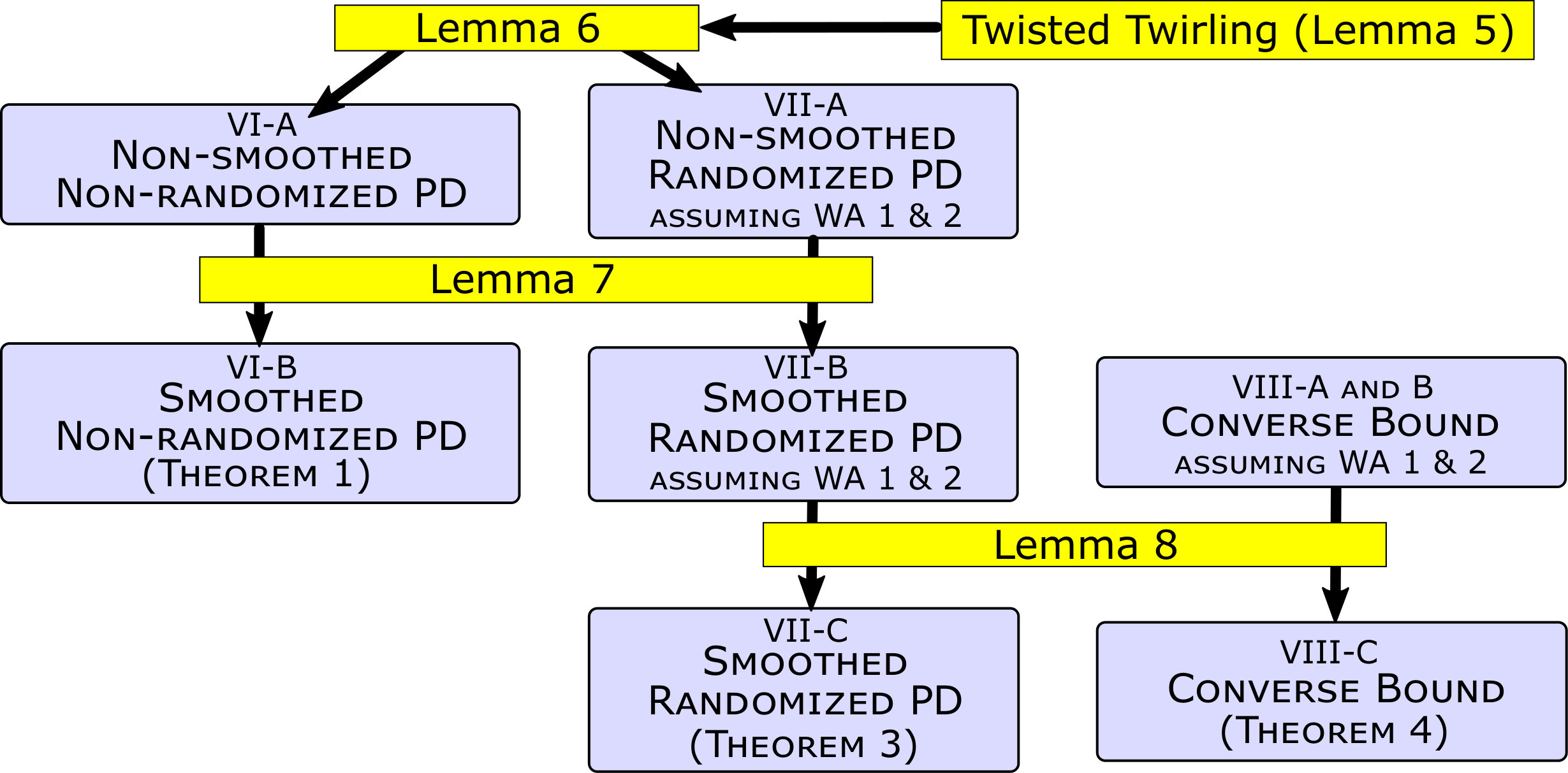 Figure 1
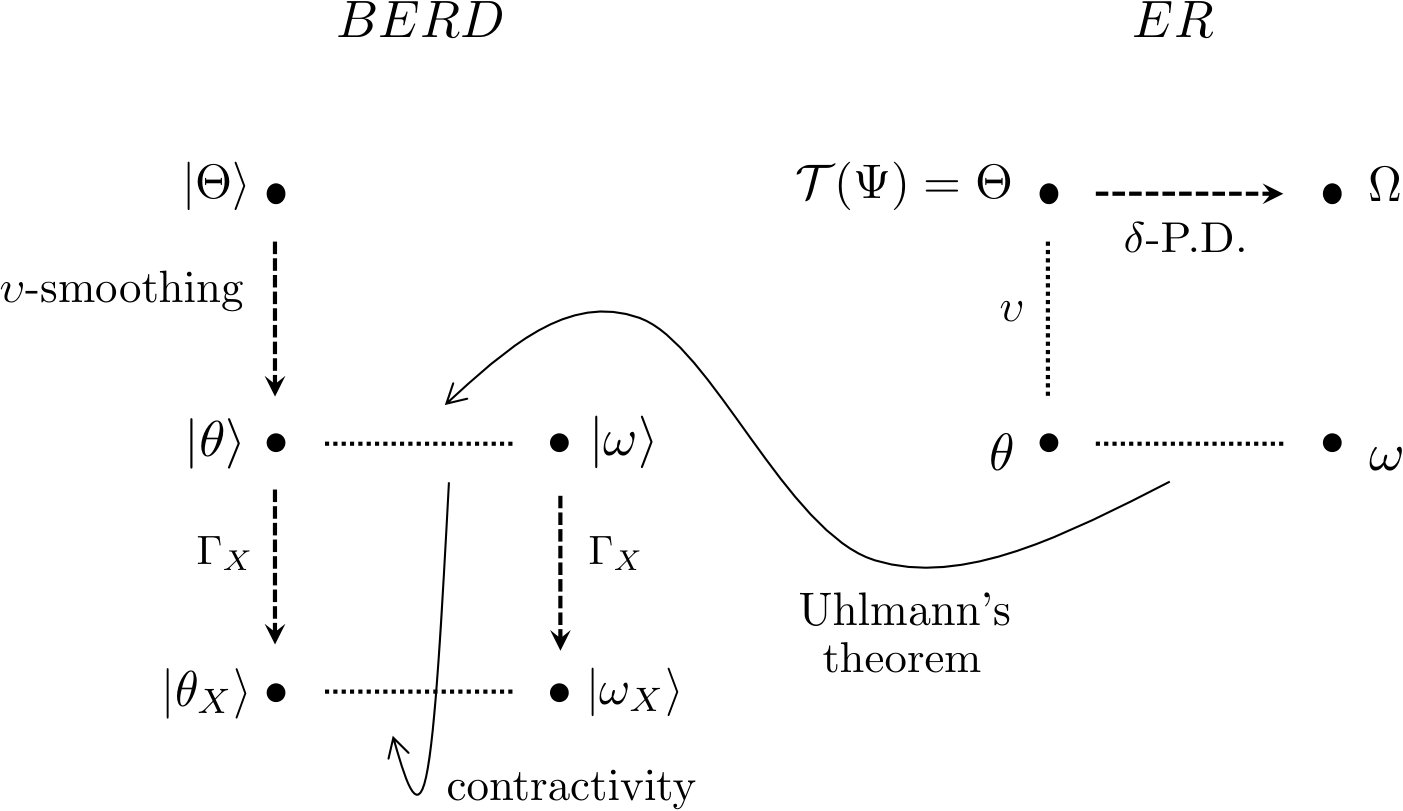 Figure 2
| General notation | |
|---|---|
| The set of linear operators on | |
| The set of linear operators from to | |
| The set of CP maps from to | |
| The set of trace non-increasing CP maps from to | |
| The set of trace preserving CP maps from to | |
| A subnormalized (resp. normalized) state on in Theorem 1 and 3 (resp. Theorem 4) | |
| A completely-positive superoperator from to (trace-preserving in Theorem 4) | |
| A complementary superoperator of | |
| Maximally entangled state between and () | |
| , | The Choi-Jamiołkowski state of and : |
| , | |
| Unitary group of degree | |
| Norms and distances | |
| The trace norm of a linear operator : | |
| The Hilbert-Schmidt norm of a linear operator : | |
| for | |
| Generalized fidelity between subnormalized states : | |
| Purified distance between subnormalized states : | |
| The -ball of a subnormalized state : | |
| Conditional Entropies for and | |
|---|---|
| for | |
| for | |
| Notations when a Hilbert space is decomposed into (Theorem 1) | |
| and | and , respectively |
| The projection onto | |
| , | Maximally entangled states on and (, ) |
| Maximally entangled state between and : | |
| A quantum system represented by a Hilbert space | |
| () | |
| A linear operator from to : | |
| An unnormalized state on : | |
| The maximally mixed state on | |
| The Haar measure on | |
| A product measure on | |
| A subnormalized state on : | |
| The DSP-diamond norm of a supermap from to : | |
Peer Reviews
No public reviews on file for this paper yet. If you reviewed it on a platform where reviews are public (OpenReview, ICLR, NeurIPS, ICML), you can paste yours below so the community can read it here.
Videos
No videos yet. Explain this paper in a talk, walkthrough, or lecture? Add one.
One-Shot Randomized and Nonrandomized Partial Decoupling
Eyuri Wakakuwa
Department of Communication Engineering and Informatics, Graduate School of Informatics and Engineering, The University of Electro-Communications, Tokyo 182-8585, Japan
Yoshifumi Nakata
Photon Science Center, Graduate School of Engineering, The University of Tokyo, Bunkyo-ku, Tokyo 113-8656, Japan
Yukawa Institute for Theoretical Physics, Kyoto university, Kitashirakawa Oiwakecho, Sakyo-ku, Kyoto, 606-8502, Japan
JST, PRESTO, 4-1-8 Honcho, Kawaguchi, Saitama, 332-0012, Japan
Abstract
We introduce a task that we call partial decoupling, in which a bipartite quantum state is transformed by a unitary operation on one of the two subsystems and then is subject to the action of a quantum channel. We assume that the subsystem is decomposed into a direct-sum-product form, which often appears in the context of quantum information theory. The unitary is chosen at random from the set of unitaries having a simple form under the decomposition. The goal of the task is to make the final state, for typical choices of the unitary, close to the averaged final state over the unitaries. We consider a one-shot scenario, and derive upper and lower bounds on the average distance between the two states. The bounds are represented simply in terms of smooth conditional entropies of quantum states involving the initial state, the channel and the decomposition. Thereby we provide generalizations of the one-shot decoupling theorem. The obtained result would lead to further development of the decoupling approaches in quantum information theory and fundamental physics.
I Introduction
Decoupling refers to the fact that we may destroy correlation between two quantum systems by applying an operation on one of the two subsystems. It has played significant roles in the development of quantum Shannon theory for a decade, particularly in proving the quantum capacity theorem HHWY2008 , unifying various quantum coding theorems ADHW2009 , analyzing a multipartite quantum communication task horo05 ; HOW07 and in quantifying correlations in quantum states GPW2005 ; berta2018conditional . It has also been applied to various fields of physics, such as the black hole information paradox HP2007 , quantum many-body systems brandao2015exponential and quantum thermodynamics dRARDV2011 ; dRHRW2014 . Dupuis et al. DBWR2010 provided one of the most general formulations of decoupling, which is often referred to as the decoupling theorem. The decoupling approach simplifies many problems of our interest, mostly due to the fact that any purification of a mixed quantum state is convertible to another reversibly uhlmann1976transition .
All the above studies rely on the notion of random unitary, i.e., unitaries drawn at random from the set of all unitaries acting on the system, which leads to the full randomization over the whole Hilbert space. In various situations, however, the full randomization is a too strong demand. In the context of communication theory, for example, the full randomization leads to reliable transmission of quantum information, while we may be interested in sending classical information at the same time devetak2005capacity , for which the full randomization is more than necessary. In the context of quantum many-body physics, the random process caused by the complexity of dynamics is in general restricted by symmetry, and thus no randomization occurs among different values of conserved quantities. Hence, in order that the random-unitary-based method fits into broader context in quantum information theory and fundamental physics, it would be desirable to generalize the previous studies using the full-random unitary, to those based on random unitaries that are not fully random but with a proper structure.
As the first step toward this goal, we consider a scenario in which the unitaries take a simple form under the following direct-sum-product (DSP) decomposition of the Hilbert space:
[TABLE]
Here, the superscripts and stand for “left” and “right”, respectively, and is the index of the diagonal subspaces. This decomposition often appears in the context of quantum information theory, such as information-preserving structure robin10 ; robin08 , the Koashi-Imoto decomposition koashi02 , data compression of quantum mixed-state source mixcomp1 , quantum Markov chains hayden04 ; wakakuwa2017markovianizing and simultaneous transmission of classical and quantum information devetak2005capacity . Also, quantum systems with symmetry are represented by the Hilbert spaces decomposed into this form (see e.g. bartlett07 ), in which case is the label of irreducible representations of a compact group , is the representation space and is the multiplicity space for each .
In this paper, we introduce and analyze a task that we call partial decoupling. We consider a scenario in which a bipartite quantum state on system is subject to a unitary operation on , followed by the action of a quantum channel (CP map) . The unitary is assumed to be chosen at random, not from the set of all unitaries on , but from the subset of unitaries that take a simple form under the DSP decomposition. Thus, partial decoupling is a generalization of the decoupling theorem DBWR2010 that incorporates the DSP decomposition. Along the similar line as DBWR2010 , we analyze how close the final state is, on average over the unitaries, to the averaged final state .
The main result in this paper is that we derive upper and lower bounds on the average distance between the final state and the averaged one. The bounds are represented in terms of the smooth conditional entropies of quantum states involving the initial state, the channel and the decomposition. For a particular case where and , the obtained formulae are equivalent to those given by the decoupling theorem DBWR2010 .
The result in this paper is applicable for generalizing any problems within the scope of the decoupling theorem by incorporating the DSP structure. Some of the applications are investigated in our papers wakakuwa2020randomized ; nakata2020one ; wakakuwa2020oneshothybrid ; nakata2020black .
In Refs. wakakuwa2020randomized ; wakakuwa2020oneshothybrid ; nakata2020one , we investigate communication tasks between two parties in which the information to be transmitted has both classical and quantum components. In this case, the Hilbert space in (1) is assumed to be a one-dimensional space , and to be the spaces with the same dimension for all :
[TABLE]
Here, and correspond to the degrees of freedom related to classical and quantum components of the information to be transmitted, respectively. We investigate the tasks of channel coding in wakakuwa2020randomized ; nakata2020one and source coding in wakakuwa2020oneshothybrid in the one-shot regime. Based on the result in this paper, we obtain general trade-off relations among the resources of classical communication, quantum communication and entanglement for those tasks.
In Ref. nakata2020black , we apply the result of partial decoupling to investigate the information paradox of quantum black holes with symmetry. Our analysis is based on the framework of Hayden-Preskill model HP2007 , where a decoupling technique is used under the postulate that the internal dynamics of the system is given by a fully random unitary. This postulate should be modified when the system has symmetry since the dynamics cannot be fully random due to a conserved quantity. By letting be the labeling of the conserved quantity, the internal dynamics randomizes only the multiplicity spaces and should be in the form of
[TABLE]
where is the identity on and is a random unitary on . Hence, this case is also in the scope of partial decoupling with a DSP decomposition given by the symmetry. Similarly, all physical phenomena investigated based on decoupling HP2007 ; brandao2015exponential ; dRARDV2011 ; dRHRW2014 ; DBWR2010 can be lifted up by partial decoupling to the situation with symmetry. We think that further significant implications on various topics will be obtained beyond these examples.
This paper is organized as follows. In Section II, we introduce notations and definitions. In Section III, we present formulations of the problem and the main results. Before we prove our main results, we provide discussions about implementations of our protocols by quantum circuits in Section IV. Section V describes the structure of the proofs of the main results, and provides lemmas that will be used in the proofs. The detailed proofs of the main theorems are provided in Section VI-VIII. Conclusions are given in Section IX. Some technical lemmas and proofs are provided in Appendices.
II Preliminaries
We summarize notations and definitions that will be used throughout this paper. See also Appendix H for the list of notations.
II.1 Notations
We denote the set of linear operators and that of Hermitian operators on a Hilbert space by and , respectively. For positive semidefinite operators, density operators and sub-normalized density operators, we use the following notations, respectively:
[TABLE]
A Hilbert space associated with a quantum system is denoted by , and its dimension is denoted by . A system composed of two subsystems and is denoted by . When and are linear operators on and , respectively, we denote as for clarity. In the case of pure states, we often abbreviate as . For , represents . We denote simply by . The maximally entangled state between and , where , is denoted by \mbox{|\Phi\rangle}^{AA^{\prime}} or . The identity operator is denoted by . We denote (M^{A}\otimes I^{B})\mbox{|\psi\rangle}^{AB} as M^{A}\mbox{|\psi\rangle}^{AB}, and as .
When is a supermap from to , we denote it by . When , we use for short. We also denote by . The set of linear completely-positive (CP) supermaps from to is denoted by , and the subset of trace non-increasing (resp. trace preserving) ones by (resp. ). When a supermap is given by a conjugation of a unitary or an isometry , we especially denote it by its calligraphic font such as
[TABLE]
Let be a quantum system such that the associated Hilbert space is decomposed into the DSP form as
[TABLE]
For the dimension of each subspace, we introduce the following notation:
[TABLE]
We denote by the projection onto a subspace for each . For any quantum system and any , we introduce a notation
[TABLE]
which leads to .
II.2 Norms and Distances
For a linear operator , the trace norm is defined as , and the Hilbert-Schmidt norm as . The trace distance between two unnormalized states is defined by . For subnormalized states , the generalized fidelity and the purified distance are defined by
[TABLE]
respectively tomamichel2010duality . The epsilon ball of a subnormalized state is defined by
[TABLE]
For a linear superoperator , we define the DSP norm by
[TABLE]
where the supremum is taken over all finite dimensional quantum systems and all subnormalized states such that the reduced state on is decomposed in the form of
[TABLE]
Here, is a probability distribution, is a set of subnormalized states on and is the maximally mixed state on . The epsilon ball of linear CP maps with respect to the DSP norm is defined by
[TABLE]
For quantum systems , , a linear operator and a subnormalized state , we introduce the following notation:
[TABLE]
This includes the case where is a trivial (one-dimensional) system, in which case . We omit the superscript for when there is no fear of confusion.
II.3 One-shot entropies
For any subnormalized state and normalized state , define
[TABLE]
The conditional min-, max- and collision entropies (see e.g. T16 ) are defined by
[TABLE]
respectively. The smoothed versions are of the key importance when we are interested in the one-shot scenario. We particularly use the smooth conditional min- and max-entropies:
[TABLE]
for . Note that Expressions (17)-(22) can be generalized to the case where .
II.4 Choi-Jamiolkowski representation
Let be a linear supermap from to , and let be the maximally entangled state between and . A linear operator defined by is called the Choi-Jamiołkowski representation of J1972 ; C1975 . The representation is an isomorphism. The inverse map is given by, for an operator ,
[TABLE]
where denotes the transposition of with respect to the Schmidt basis of . When is completely positive, then is an unnormalized state on and is called the Choi-Jamiołkowski state of .
Note that the Choi-Jamiołkowski representation depends on the choice of the maximally entangled state , i.e., the Schmidt basis thereof. When is decomposed into the DSP form as (8), the isomorphic space is decomposed into the same form. In the rest of this paper, we fix the maximally entangled state , which is decomposed as
[TABLE]
where and are fixed maximally entangled states on and , respectively.
II.5 Random unitaries
Random unitaries play a crucial role in the analyses of one-shot decoupling. By using them, it can be shown that there exists at least one unitary that achieves the desired task. In particular, the Haar measure on the unitary group is often used. The Haar measure on the unitary group is the unique unitarily invariant provability measure, often called uniform distribution of the unitary group. When a random unitary is chosen uniformly at random with respect to the Haar measure, it is referred to as a Haar random unitary and is denoted by .
The most important property of the Haar measure is the left- and right-unitary invariance: for a Haar random unitary and any unitary , the random unitaries and are both distributed uniformly with respect to the Haar measure. This property combined with the Schur-Weyl duality enables us to explicitly study the averages of many functions on the unitary group over the Haar measure. In the following, the average of a function on the unitary group over the Haar measure is denoted by .
In this paper, however, we are interested in the case where the Hilbert space is decomposed into the DSP form: , and mainly consider the unitaries that act non-trivially only on such as the untiary in the form of , where is a unitary on . In this case, we can naturally introduce a product of the Haar measures by
[TABLE]
where is the Haar measure on the unitary group on for any . Hence, when we write below, it means that is in the form of and .
III Main Results
We consider two scenarios in which a bipartite quantum state is transformed by a unitary operation on and then is subject to the action of a quantum channel (linear CP map) . The unitary is chosen at uniformly random from the set of unitaries that take a simple form under the DSP decomposition (1).
In the first scenario, which we call non-randomized partial decoupling, the unitaries are such that they completely randomize the space for each , while having no effect on or the space . This scenario may find applications when complex quantum many-body systems are investigated based on the decoupling approach, in which case the DSP decomposition is, for instance, induced by the symmetry the system has. In the second scenario, which we refer to as randomized partial decoupling, we assume that and that does not depend on . The unitaries do not only completely randomize the space , but also randomly permute . This scenario may fit to the communication problems. For instance, one of the applications may be classical-quantum hybrid communicational tasks, where the division of the classical and quantum information leads to the DSP decomposition.
For both scenarios, our concern is how close the final state is, after the action of the unitary and the quantum channel, to the averaged final state over all unitaries. It should be noted that the averaged final state is in the form of a block-wise decoupled state in general. This is in contrast to the decoupling theorem, in which the averaged final state is a fully decoupled state.
III.1 Non-Randomized Partial Decoupling
Let us consider the situation where has the DSP form: . For any state , the averaged state obtained after the action of the random unitary is given by
[TABLE]
Here, is the maximally mixed state on , and is an unnormalized state on defined by
[TABLE]
Our interest is on the average distance between the state and the averaged state over all .
For expressing the upper bound on the average distance, we introduce a quantum system represented by a Hilbert space
[TABLE]
and a linear operator defined by
[TABLE]
where , and .
The following is our first main theorem about the upper bound:
** Theorem 1**
*[Main result 1: One-shot non-randomized partial decoupling] For any , any subnormalized state and any linear CP map , it holds that *
[TABLE]
Here, is the smooth conditional min-entropy for an unnormalized state , defined by with being the Choi-Jamiołkowski representation of . It is explicitly given by
[TABLE]
where is the set of -neighbourhoods of , defined by (15).
In the literature of chaotic quantum many-body systems, it is often assumed that the dynamics is approximated well by a random unitary channel, which is sometimes called scrambling HP2007 ; SS2008 ; LSHOH2013 . Despite the fact that a number of novel research topics have been opened based on the idea of scrambling, some of which are using the decoupling approach HP2007 ; dRARDV2011 ; dRHRW2014 , symmetry of the physical systems has rarely been taken into account properly. When the system has symmetry, the associated Hilbert space is naturally decomposed into a DSP form as
[TABLE]
where is the label of irreducible representations of a compact group of the symmetry, is the irreducible representation and corresponds to the multiplicity for each . Due to the conservation law, the scrambling dynamics in the system should be compatible with this decomposition and should be in the form of . Hence, Theorem 1 is applicable to the study of complex physics in chaotic quantum many-body systems with symmetry.
Theorem 1 reduces to a simpler form when the symmetry is abelian. In this case, all the irreducible representation one-dimensional, i.e., . The averaged output state is explicitly calculated to be
[TABLE]
The operator in (31) reduces to a direct sum of operators that are proportional to projectors, and the operator in Theorem 1 reduces to
[TABLE]
Theorem 1 implies that, if the smooth conditional min-entropy of the unnormalized state is sufficiently large, the final state is close to .
III.2 Randomized Partial Decoupling
Next we assume that
[TABLE]
The Hilbert space is then isomorphic to a tensor product Hilbert space , i.e., . Here, is a -dimensional Hilbert space with a fixed orthonormal basis , and is an -dimensional Hilbert space. We consider a random unitary on system of the form
[TABLE]
which we also denote by . In addition, let be the permutation group on , and be the uniform distribution on . We define a unitary for any by
[TABLE]
We denote the supermap given by conjugation of by the calligraphic font as . For the initial state, we use the notion of classically coherent states, defined as follows:
** Definition 2**** **(classically coherent states dupuis2014decoupling )
Let and be -dimensional quantum systems with fixed orthonormal bases and , respectively, and let be a quantum system. An unnormalized state is said to be classically coherent in if it satisfies \varrho\mbox{|k\rangle}^{K_{1}}\mbox{|k^{\prime}\rangle}^{K_{2}}=0 for any , or equivalently, if is in the form of
[TABLE]
where for each and .
We now provide our second main result:
** Theorem 3**
[Main result 2: One-shot randomized partial decoupling] Let , be a subnormalized state that is classically coherent in , and be a linear CP map such that the Choi-Jamiołkowski representation satisfies . It holds that
[TABLE]
where . The function is [math] for and for , and is [math] for and for . The exponents and are given by
[TABLE]
Here, is the completely dephasing channel on with respect to the basis , and is the Choi-Jamiolkowski representation of the complementary channel of .
Note that, since the subnormalized state is classically coherent in , the averaged state is explicitly given by
[TABLE]
Small error for one-shot randomized partial decoupling implies that the third party having the purifying system of the final state may recover both classical and quantum parts of correlation in . Thus, it will be applicable, e.g., for analyzing simultaneous transmission of classical and quantum information in the presence of quantum side information. In this context, in the above expression quantifies how well the total correlation in can be transmitted by the channel , whereas for only quantum part thereof (see wakakuwa2020randomized ; wakakuwa2020oneshothybrid ; nakata2020one ).
III.3 A Converse Bound
So far, we have presented achievabilities of non-randomized and randomized partial decoupling. At this point, we do not know whether the obtained bounds are “sufficiently tight”. To address this question, we prove a converse bound for partial decoupling. We assume the following two conditions for the converse:
- Converse Condition 1
,
- Converse Condition 2
the initial (normalized) state is classically coherent in .
Throughout the paper, we refer to the conditions as CC1 and CC2, respectively. The two conditions are always satisfied in the case of randomized partial decoupling, but not necessarily satisfied in the case of non-randomize one. Consequently, the converse bound we prove below is directly applicable to randomized partial decoupling, but is not applicable to non-randomized partial decoupling in general.
The converse bound is stated by the following theorem.
** Theorem 4**
[Main result 3: Converse for partial decoupling] Suppose that CC1 and CC2 are satisfied. Let be a purification of a normalized state , which is classically coherent in due to CC2, and be a trace preserving CP map with the complementary channel . Suppose that, for , there exists a normalized state \Omega^{ER}:=\sum_{j=1}^{J}\varsigma_{j}^{E}\otimes\Psi_{jj}^{R_{r}}\otimes\mbox{\mbox{}!\mbox{}}^{R_{c}}, where are normalized states on , such that
[TABLE]
Then, for any and , it holds that
[TABLE]
where is the completely dephasing channel on , and the smoothing parameters and are defined by
[TABLE]
and .
Note that, when a quantum channel achieves partial decoupling for a state within a small error, it follows from the decomposition of (see (43)) that
[TABLE]
where \hat{\tau}_{j}^{E}:={\mathcal{T}}^{A\rightarrow E}(\mbox{\mbox{}!\mbox{}}^{A_{c}}\otimes\pi^{A_{r}})=({\mathcal{H}}^{E}). This is in the same form as the assumption of Theorem 4.
Let us compare the direct part of randomized partial decoupling (Theorem 3) and the converse bound presented above. The first term in the R.H.S. of the achievability bound (41) is calculated to be
[TABLE]
On the other hand, the converse bound (45) yields
[TABLE]
where , with being a purification of and . Note that there exists a linear isometry from to that maps to uhlmann1976transition , and that the conditional max entropy is invariant under local isometry (see Lemma 21 below). A similar argument also applies to the second term in (41) and (46). Thus, when is the maximally mixed state, in which case and thus , the gap between the two bounds is only due to the difference in values of smoothing parameters and types of conditional entropies. By the fully quantum asymptotic equipartition property tomamichel2009fully , this gap vanishes in the limit of infinitely many copies. From this viewpoint, we conclude that the achievability bound of randomized partial decoupling and the converse bound are sufficiently tight.
III.4 Reduction to The Existing Results
We briefly show that the existing results on one-shot decoupling DBWR2010 and dequantization dupuis2014decoupling are obtained from Theorems 1, 3 and 4 as corollaries, up to changes in smoothing parameters. Thus, our results are indeed generalizations of these two tasks.
First, by letting in Theorem 3, we obtain the achievability of one-shot decoupling:
** Corollary 5**
[Achievability for one-shot decoupling (Theorem 3.1 in DBWR2010 )] Let , be a subnormalized state, and be a linear CP map such that the Choi-Jamiołkowski representation satisfies . Let be the Haar random unitary on . Then, it holds that
[TABLE]
Note that the duality of the conditional min and max entropies (tomamichel2010duality : see also Lemma 24 in Section V.2.2) implies , with being the Choi-Jamiolkowski representation of the complementary channel of . A similar bound is also obtained by letting and in Theorem 1. A converse bound for one-shot decoupling is obtained by letting in Theorem 4, and by using the duality of the conditional entropies, as follows:
** Corollary 6**
[Converse for one-shot decoupling (Theorem 4.1 in DBWR2010 )] Consider a normalized state and a trace preserving CP map . Suppose that, for , there exists a normalized state , such that . Then, for any and , it holds that
[TABLE]
where is a purification of , , and the smoothing parameter is defined by (47).
Next, we consider the opposite extreme for Theorem 3, i.e., we consider the case where . This case yields the dequantizing theorem:
** Corollary 7**
[Achievability for dequantization (Theorem 3.1 in dupuis2014decoupling )] Let be a quantum system with a fixed basis , and . Consider a subnormalized state that is classically coherent in , and a linear CP map such that the Choi-Jamiołkowski representation satisfies . Let be the random permutation on with the associated unitary G_{\sigma}:=\sum_{j=1}^{d_{A}}\mbox{\mbox{}!\mbox{}}. Then, it holds that
[TABLE]
where is the completely dephasing channel on with respect to the basis , and is the Choi-Jamiolkowski representation of the complementary channel of .
In the same extreme, Theorem 4 provides a converse bound for dequantization, which has not been known so far:
** Corollary 8**
[Converse for dequantization] Consider the same setting as in Corollary 7, and assume that is normalized, and that is trace preserving. Let be a purification of . Suppose that, for , there exists a normalized state \Omega^{ER}:=\sum_{j=1}^{J}p_{j}\varsigma_{j}^{E}\otimes\mbox{\mbox{}!\mbox{}}^{R}, where is an ensemble of normalized states on , such that . Then, for any and , it holds that
[TABLE]
where the smoothing parameter is defined by (47).
IV Implementing the random unitary with the DSP form
Before we proceed to the proofs, we here briefly discuss how the random unitaries that respect the DSP form can be implemented by quantum circuits. Since Haar random unitaries are in general hard to implement, unitary -designs, mimicking the -th statistical moments of the Haar measure on average DLT2002 ; DCEL2009 ; GAE2007 , have been exploited in many cases. Since the decoupling method makes use of the second statistical moments of the Haar measure, we could use the unitary -designs instead of the Haar measure for our tasks. Although a number of efficient implementations of unitary -designs have been discovered DLT2002 ; BWV2008a ; WBV2008 ; GAE2007 ; DCEL2009 ; HL2009 ; DJ2011 ; CLLW2015 ; NHMW2015-1 , and it is also shown that decoupling can be achieved using unitaries less random than unitary 2-designs BF2013 ; NHMW2015-2 , we here need unitary designs in a given DSP form, which we refer to as the DSP unitary designs. Thus, we cannot directly use the existing constructions, posing a new problem about efficient implementations of DSP unitary designs. Although this problem is out of the scope in this paper, we will briefly discuss possible directions toward the solution.
One possible way is to simply modify the constructions of unitary designs known so far. This could be done by regarding each Hilbert space , on which each random unitary acts, as the Hilbert space of “virtual” qubits. The complexity of the implementation, i.e. the number of quantum gates, is then determined by how complicated the unitary is that transforms the basis in each into the standard basis of the virtual qubits. Another way is to use the implementation of designs on one qudit NHKW2017 , where it was shown that alternate applications of random diagonal unitaries in two complementary bases achieves unitary designs. This implementation would be suited in quantum many-body systems because we can choose two natural bases, position and momentum bases, and just repeat switching random potentials in those bases under the condition that the potentials satisfy the DSP form. Finally, when the symmetry-induced DSP form is our concern, unitary designs with symmetry may possibly be implementable by applying random quantum gates that respects the symmetry.
In any case, the implementations of DSP unitary designs, or the symmetric unitary designs, and their efficiency are left fully open. Further analyses are desired.
V Structure of the Proof
In the rest of the paper, we prove the three main theorems, Theorem 1, Theorem 3 and Theorem 4 in Section VI, Section VII and Section VIII, respectively. For the sake of clarity, we sketch the outline of the proofs in Subsection V.1 (see also Fig. 1). We then list useful lemmas in Subsection V.2. See also Appendix H for the list of notations used in the proofs.
V.1 Key lemmas and the structure of the proofs
For the achievability statements (Theorem 1 and Theorem 3), the key technical lemma is the twisted twirling, which can be seen as a generalization of the twirling method often used in quantum information science. See Appendix A for the proof.
** Lemma 9**** **(Twisted Twirling)
Let be a -dimensional subspace of , and be the projector onto for each of . Let be , and be the swap operator defined by for any orthonormal basis \{\mbox{|a\rangle}\} in and . In addition, let and be and , respectively. For any , define
[TABLE]
Then, it holds that, for ,
[TABLE]
Moreover,
[TABLE]
Otherwise, {\mathbb{E}}_{U_{j},U_{k},U_{m},U_{n}}\bigl{[}(U_{j}^{A_{r}}\otimes U_{k}^{A_{r}^{\prime}})M^{A_{r}A_{r}^{\prime}BB^{\prime}}(U_{m}^{A_{r}}\otimes U_{n}^{A_{r}^{\prime}})^{\dagger}\bigr{]}=0.
The twisted twirling enables us to show the following lemma (see Appendix B).
** Lemma 10**
For any and any such that , the following inequality holds for any possible permutation :
[TABLE]
Here, denotes the transposition of with respect to the Schmidt basis of the maximally entangled state in (26), and the norm in the R.H.S. is defined by (16).
Based on this lemma, we can prove the non-smoothed versions of Theorem 1 and Theorem 3 in Subsections VI.1 and VII.1, respectively.
To complete the proofs of Theorem 1 and Theorem 3, smoothing the statements is needed, which is done in Subsections VI.2 and VII.2 based on the following lemma proven in Appendix C.
** Lemma 11**
Consider arbitrary unnormalized states and arbitrary CP maps . Let and be arbitrary CP maps such that . Let and be linear operators on , such that
[TABLE]
and that
[TABLE]
The following inequality holds for any possible permutation and for both and :
[TABLE]
Here, for and for .
The converse statements are proved independently in Section VIII.
When we prove the one-shot randomized decoupling theorem (Theorem 3) and the converse (Theorem 4), we first put the following two working assumptions:
WA 1
, where is a quantum system of dimension .
WA 2
The CP map is decomposed into
[TABLE]
in which is a linear supermap from to defined by {\mathcal{T}}_{jk}(\zeta)={\mathcal{T}}(\mbox{\mbox{}!\mbox{}}\otimes\zeta) for each .
These assumptions are finally dropped in Subsections VII.3 and VIII.3 using the following lemma (see Appendix D for a proof).
** Lemma 12**
Let be a linear CP map that does not necessarily satisfies WA 1 and WA 2. By introducing a quantum system with dimension , define an isometry Y^{A_{c}\rightarrow A_{c}E_{c}}:=\sum_{j}\mbox{|jj\rangle}^{A_{c}E_{c}}\mbox{\langle j|}^{A_{c}}, and a linear map by . Then, is a linear CP map and, for any that is classically coherent in , the following equalities hold:
[TABLE]
V.2 List of useful lemmas
We here provide several useful lemmas, some of which are in common with those in the proof of the one-shot decoupling theorem DBWR2010 . Proofs of Lemmas 16–20 and 29–35 will be provided in Appendix E.
V.2.1 Properties of Norms and Distances
** Lemma 13**** **(Lemma 3.6 in DBWR2010 )
For any , .
** Lemma 14**** **(Lemma 3.7 in DBWR2010 )
For any and , it holds that
[TABLE]
** Lemma 15**** **(Sec. II in tomamichel2010duality )
The purified distance defined by (11) satisfies the following properties:
triangle inequality: For any , it holds that . 2. 2.
monotonicity: For any and trace-nonincreasing CP map , it holds that . 3. 3.
Uhlmann’s theorem: For any and any purification of , where , there exists a purification of such that .
** Lemma 16**
The purified distance defined by (11) satisfies the following properties:
pure states: For any subnormalized pure state and any normalized pure state , . 2. 2.
relation to the trace distance: For any , . 3. 3.
Inequality for subnormalized pure states: For any subnormalized pure states \mbox{|\psi\rangle},\mbox{|\phi\rangle}\in{\mathcal{H}}, P(\psi,\phi)\leq\sqrt{1-|\mbox{\left\langle\psi|\phi\right\rangle}|^{2}}+\sqrt{1-\mbox{\left\langle\phi|\phi\right\rangle}}.
** Lemma 17**
Let be a normalized probability distribution, be a set of normalized states on , and be that of subnormalized ones. For \rho^{ABK}:=\sum_{k}p_{k}\rho_{k}^{AB}\otimes\mbox{\mbox{}!\mbox{}}^{K} and \hat{\rho}^{ABK}:=\sum_{k}p_{k}\hat{\rho}_{k}^{AB}\otimes\mbox{\mbox{}!\mbox{}}^{K}, the purified distance satisfies
[TABLE]
** Lemma 18**
Let and be subnormalized probability distributions, and and be sets of normalized states on . For \rho^{AK}:=\sum_{k}p_{k}\rho_{k}^{A}\otimes\mbox{\mbox{}!\mbox{}}^{K} and \varsigma^{AK}:=\sum_{k}q_{k}\varsigma_{k}^{A}\otimes\mbox{\mbox{}!\mbox{}}^{K}, it holds that
[TABLE]
** Lemma 19**
*The DSP norm defined by (13) satisfies the triangle inequality, i.e., for any superoperators and from to , . *
** Lemma 20**
Let be a set of orthogonal projectors on such that . For any , .
V.2.2 Properties of Conditional Entropies
** Lemma 21**** **(Corollary of Lemma 13 in tomamichel2010duality )
For any , and any linear isometry , .
** Lemma 22**** **(Corollary of Lemma 15 in tomamichel2010duality )
For any , and any linear isometry , .
** Lemma 23**** **(Lemma A.1 in DBWR2010 )
For any and , it holds that
[TABLE]
** Lemma 24**** **(Definition 14, Equality (6) and Lemma 16 in tomamichel2010duality )
For any subnormalized pure state on system , and for any , .
** Lemma 25**** **(Lemma B.2 in DBWR2010 )
Let be a subnormalized pure state. For any full-rank state , it holds that , where
[TABLE]
** Lemma 26**** **(Lemma A.5 in DBWR2010 )
For any state in the form of
[TABLE]
where , \mbox{\left\langle k|k^{\prime}\right\rangle}=\delta_{k,k^{\prime}} and is a normalized probability distribution, it holds that
[TABLE]
(It is straightforward to show that the above equalities also hold for and , by noting that and that .)
** Lemma 27**** **(Lemma A.7 in DBWR2010 )
For any state in the form of
[TABLE]
where the notations are the same as in Lemma 26, and for any it holds that
[TABLE]
(Note that, although Lemma A.7 in DBWR2010 assumes that is normalized, the condition is not used in the proof thereof.)
** Lemma 28**** **(Lemma A.1 in dupuis2014decoupling )
Let be a subnormalized state that is classically coherent in . For any , there exists that is classically coherent in , and that is decomposed as \varsigma=\sum_{k}\mbox{\mbox{}!\mbox{}}^{K_{2}}\otimes\varsigma_{k}^{B}, such that
[TABLE]
** Lemma 29**
In the same setting as in Lemma 27, it holds that
[TABLE]
** Lemma 30**
Let be a subnormalized state that is classically coherent in . For any , there exists that is classically coherent in , such that
[TABLE]
If is also diagonal in (i.e., if is in the form of (75)), there exists , satisfying the above conditions, that is diagonal in .
** Lemma 31**
Consider the same setting as in Lemma 26. For any such that , it holds that
[TABLE]
where .
V.2.3 Other Technical Lemmas
** Lemma 32**
Consider two linear operators and assume that , . Let \mbox{|\Phi\rangle}^{AA^{\prime}} and \mbox{|\Phi\rangle}^{BB^{\prime}} be maximally entangled states between and , and and , respectively. Then, {\rm Tr}[X^{T}Y]=\sqrt{d_{A}d_{B}}\mbox{\langle\Phi|}^{BB^{\prime}}(X\otimes Y)\mbox{|\Phi\rangle}^{AA^{\prime}}, where , and the transposition is taken with respect to the Schmidt bases of \mbox{|\Phi\rangle}^{AA^{\prime}} and \mbox{|\Phi\rangle}^{BB^{\prime}}.
** Lemma 33**
If is classically coherent in for a positive semidefinite operator , so is .
** Lemma 34**
Let be the maximally mixed state on system , and let be the completely dephasing operation on with respect to a fixed basis . For any , it holds that
[TABLE]
** Lemma 35**
For subnormalized pure states \mbox{|\psi\rangle},\mbox{|\phi\rangle}\in{\mathcal{H}} and a real number , suppose that there exists a normalized pure state \mbox{|e\rangle}\in{\mathcal{H}} that satisfies \mbox{\left\langle e|\psi\right\rangle}\geq c and \mbox{\left\langle e|\phi\right\rangle}\geq c. Then, |\mbox{\left\langle\psi|\phi\right\rangle}|\geq 2c^{2}-1.
** Lemma 36**
(Lemma 35 in wakakuwa2017coding ) Let be a constant, be a monotonically nondecreasing function that satisfies , and be a probability distribution on a countable set . Suppose satisfies , and for a given . Then we have
[TABLE]
VI Proof of The Non-Randomized Partial Decoupling (Theorem 1)
We now prove the non-randomized partial decoupling (Theorem 1). As sketched in Subsection V.1, we proceed the proof in two steps: showing the non-smoothed version in Subsection VI.1, and then smoothing it in Subsection VI.2.
VI.1 Proof of The Non-Smoothed Non-randomized Partial Decoupling
The non-smoothed version of Theorem 1 is given by
[TABLE]
where . Note that, due to the definition of the conditional collision entropy (19), (22) and its relation to the conditional min-entropy (see Lemma 23), we have
[TABLE]
for a proper choice of . In addition, it holds that
[TABLE]
We first show this relation.
Let be the projection onto a subspace for each . Due to the definition of given by (31), it holds that
[TABLE]
Using the property of the Hilbert-Schmidt norm (Lemma 20), we have
[TABLE]
Using Eq. (87) and the explicit form of , i.e. , each term in the summand is given by
[TABLE]
where the last line follows from Lemma 32. Thus, we obtain (86).
From Eqs. (85) and (86), it suffices to prove that
[TABLE]
for any . In the following, we denote the L.H.S. of Ineq. (90) by . Due to Lemma 14, for any , we have
[TABLE]
Using this and Jensen’s inequality, we obtain
[TABLE]
Noting that , we can apply Lemma 10 for and . This yields
[TABLE]
where the second line follows from the fact that for . To calculate the first term in (93), note that
[TABLE]
and that
[TABLE]
Thus, we simply apply Lemma 34 to obtain
[TABLE]
for each . Substituting this to (93), we arrive at Ineq. (90).
VI.2 Proof of The Smoothed Non-Randomized Partial Decoupling
We now smoothen the conditional min-entropy to complete the proof of Theorem 1. To this end, fix and so that
[TABLE]
Let be a purification of . Noting that is decomposed in the form of (28), by properly choosing a DSP decomposition for , it holds that
[TABLE]
where and is a purification of for each . Let and be linear operators on such that and that
[TABLE]
In addition, let and be superoperators such that
[TABLE]
which yields . Note that, in general, it does not necessarily imply that and .
We now apply Lemma 11 for the case where . To obtain the explicit forms, we compute
[TABLE]
where we have used the properties of , , and described above. The last line follows from the definition of the DSP norm. Furthermore, introducing a notation , we also have (see Lemma 11 for the definition and properties of )
[TABLE]
where the fourth line follows from the definition of the DSP norm (13), and the seventh line from the triangle inequality for the DSP norm (Lemma 19). Applying the non-smoothed version of the non-randomized partial decoupling (Ineq. (84)) to a state and a CP map , we have
[TABLE]
All together, Ineq. (63) in Lemma 11 leads to
[TABLE]
which, together with (97), concludes the proof of Theorem 1.
VII Proof of The Randomized Partial Decoupling (Theorem 3)
We here show Theorem 3. We first put the following two assumptions, which simplify the proof:
WA 1
, where is a quantum system of dimension
WA 2
The CP map is decomposed into
[TABLE]
in which is a linear supermap from to defined by {\mathcal{T}}_{jk}(\zeta)={\mathcal{T}}(\mbox{\mbox{}!\mbox{}}\otimes\zeta) for each .
We show the non-smoothed version in Subsection VII.1 and the smoothed version in Subsection VII.2. The above assumptions are then dropped in Subsection VII.3.
VII.1 Proof of The Non-Smoothed Randomized Partial Decoupling under WA 1 and WA 2
Under the assumptions WA 1 and WA 2, the non-smoothed version of the randomized partial decoupling is given by
[TABLE]
Note that, as we will describe in Subsection VII.3 for general cases, the min entropies and are equal to the max entropies and , respectively, due to the duality of the conditional entropies for pure states (Lemma 24). The proof of this inequality will be divided into three steps.
VII.1.1 Upper bound on the average trace norm
To prove Ineq. (106), we first introduce the following lemma that relates the average trace norm of an operator to the average Hilbert-Schmidt norm.
** Lemma 37**
Let be an arbitrary Hermitian operator such that X^{AR}=\sum_{j,k=1}^{J}\mbox{\mbox{}!\mbox{}}^{A_{c}}\otimes X_{jk}^{A_{r}R_{r}}\otimes\mbox{\mbox{}!\mbox{}}^{R_{c}}, and let and be arbitrary states that are decomposed as \zeta^{E}\!=\!\sum_{j}\mbox{\mbox{}!\mbox{}}^{E_{c}}\!\otimes\zeta_{j}^{E_{r}}, \xi^{R}\!=\!\sum_{j}\mbox{\mbox{}!\mbox{}}^{R_{c}}\!\otimes\xi_{j}^{R_{r}}, respectively. Then it holds that
[TABLE]
where the norm in the R.H.S. is defined by (16).
It should be noted that Lemma 37 provides a stronger inequality than that obtained simply using Lemma 14.
** Proof: **
We exploit techniques developed in dupuis2014decoupling . Recall that is in the form of \sum_{j=1}^{J}\mbox{\mbox{}!\mbox{}}^{A_{c}}\otimes U_{j}^{A_{r}}, and is defined by G_{\sigma}:=\sum_{j=1}^{J}\mbox{\mbox{}!\mbox{}}^{A_{c}}\otimes I^{A_{r}} for any .
We define a subnormalized state for each by \gamma_{\sigma}^{ER}:=\sum_{j=1}^{J}\mbox{\mbox{}!\mbox{}}^{E_{c}}\otimes\zeta_{\sigma(j)}^{E_{r}}\otimes\xi_{j}^{R_{r}}\otimes\mbox{\mbox{}!\mbox{}}^{R_{c}}. Further, by letting be a quantum system with an orthonormal basis , we define a subnromalized state by
[TABLE]
Using Lemma 14 and Jensen’s inequality, we obtain
[TABLE]
In the last line, we used the following relation:
[TABLE]
which can be observed from the fact that, due to the decomposition of from WA 2,
[TABLE]
Due to the fact that
[TABLE]
for all , we obtain
[TABLE]
Substituting this to (109), and by using Jensen’s inequality, we arrive at the desired result.
VII.1.2 Generalization of the dequantizing theorem
Our second step to prove the non-smoothed randomized partial decoupling is to generalize the non-smoothed version of the dequantizing theorem (Proposition 3.5 in dupuis2014decoupling ).
** Lemma 38**
In the same setting as in Theorem 3, it holds that
[TABLE]
where we have defined \Psi_{\rm dp}^{AR}:={\mathcal{C}}^{A}(\Psi^{AR})=\sum_{j=1}^{J}\mbox{\mbox{}!\mbox{}}^{A_{c}}\otimes\Psi_{jj}^{A_{r}R}.
Note that is [math] for and for .
** Proof: **
Since and are classically coherent in by assumption, we can apply Lemma 37 for to obtain
[TABLE]
Noting that , we can also apply Lemma 10 under the assumption that is a one-dimensional system, and . Then, we obtain, for any ,
[TABLE]
where we have used in the last line. Taking the case of into account, and noting that for any function , it follows that
[TABLE]
Here, we have used the definitions and in the sixth line, and Lemma 34 in the seventh line. Due the relation between the conditional collision entropy and the conditional min-entropy (Lemma 23), it is further bounded from above by .
Finally, we use the property of the the conditional min-entropy (Lemma 28). There exist normalized states and in the form of
[TABLE]
such that and . Thus, we obtain
[TABLE]
which, together with Ineq. (115), complete the proof of Lemma 38.
VII.1.3 Proof of The Non-Smoothed Randomized Partial Decoupling
We now prove the non-smoothed randomized partial decoupling, i.e.,
[TABLE]
under the assumptions WA 1 and WA 2. Note that is [math] for and for . By the triangle inequality, we have
[TABLE]
where we have used the fact that the unitary invariance of the Haar measure implies for any unitary . The first term is bounded by simply using Lemma 38.
To bound the second term in (121), we use Lemma 37, leading to
[TABLE]
Since by definition, we can apply Lemma 10 for . Noting that for , this yields
[TABLE]
Thus, similarly to the derivation around Eq. (117), we obtain
[TABLE]
Substituting this into Ineq. (122), and noting that if , we obtain an upper bound on the second term of the R.H.S. in Ineq. (121).
All together, we obtain Ineq. (120) as desired.
VII.2 Proof of The Randomized Partial Decoupling under The Conditions WA 1 and WA 2
We now show, under the conditions WA 1 and WA 2, the randomized partial decoupling:
[TABLE]
where . The function is [math] for and for , and is [math] for and for . The exponents and are given by
[TABLE]
Note that, the duality of the conditional smooth entropies for pure states (Lemma 24), implies and (see Subsection VII.3 for the detail).
To prove the statement, we again start with the triangle inequaltiy: By the triangle inequality, we have
[TABLE]
Below, we derive upper bounds on the two terms in the R.H.S. separately.
For an upper bound on the first term, fix and so that we have and . Let and be linear operators on such that
[TABLE]
and that
[TABLE]
Let and be superoperators such that
[TABLE]
which yields . From Lemma 11, the CP map having the Choi-Jamiołkowski state satisfies
[TABLE]
Due to Lemma 38, the first term in the R.H.S. of the above inequality is bounded as
[TABLE]
Similarly to (101) and (102), using (128) and (129), it turns out that the second and the third terms are bounded from above by
[TABLE]
and
[TABLE]
respectively. Hence, we obtain
[TABLE]
In the same way, we also have
[TABLE]
Substituting these inequalities into Eq. (127), we obtain the desired result (Ineq. (125)).
VII.3 Dropping Working Assumptions WA 1 and WA 2
We now drop the working assumptions WA 1 and WA 2, and show that Theorem 3 holds in general. To remind the working assumptions, we write them down here again:
- WA 1
, where is a quantum system of dimension
- WA 2
The CP map is decomposed into
[TABLE]
in which is a linear supermap from to defined by {\mathcal{T}}_{jk}(\zeta)={\mathcal{T}}(\mbox{\mbox{}!\mbox{}}\otimes\zeta) for each ,
To drop these assumptions, we use Lemma 12. Using the linear isometry , given by Y=\sum_{j}\mbox{|jj\rangle}^{A_{c}E_{c}}\mbox{\langle j|}^{A_{c}}, we define a new CP map by . Lemma 12 states that
[TABLE]
Let be the Choi-Jamiołkowski state of , i.e., . We denote by a purification of such that the reduced state is equal to , where is the complementary map of . Then, it is clear that , which implies that a purification of is given by . It is also straightforward to verify that .
The new CP map clearly satisfies WA 1 and WA 2. Hence, using Eq. (138) and achievability of the randomized partial decoupling under those assumptions (Ineq. (125)), we obtain
[TABLE]
Due to the duality of conditional smooth entropies (Lemma 24), we have
[TABLE]
Using the property of the conditional smooth entropy for classical-quantum states (Lemma 27), and noting that is classically coherent in , we also have
[TABLE]
Substituting these into (139), and noting that by assumption, we obtain Theorem 3.
VIII Proof of The Converse
We provide the proof of Theorem 4 under Converse Conditions 1 and 2, which are
CC 1
,
CC 2
the initial (normalized) state is classically coherent in .
The proof proceeds along the similar line as the proof of the converse part of the one-shot decoupling theorem (see Section 4 in DBWR2010 ). Suppose that there exists a normalized state \Omega^{ER}:=\sum_{j=1}^{J}\varsigma_{j}^{E}\otimes\Psi_{jj}^{R_{r}}\otimes\mbox{\mbox{}!\mbox{}}^{R_{c}}, where are normalized states on , such that, for ,
[TABLE]
We separately prove that, in this case, the following inequalities hold for any and :
[TABLE]
Here, and are given by
[TABLE]
and .
First, we prove these relations based on the working assumptions WA 1 and WA 2 in Subsection VIII.1 and VIII.2. We complete the proof of Theorem 4 by dropping these assumptions in Subsection VIII.3.
VIII.1 Proof of Ineq. (143) under WA 1 and WA 2
To prove Ineq. (143), we introduce the following notations:
- •
\mbox{|\Psi\rangle}^{ARD} : A purification of .
- •
: A Stinespring dilation of .
- •
\mbox{|\Theta\rangle}^{BERD} : A pure state on defined by \mbox{|\Theta\rangle}:=V\mbox{|\Psi\rangle}.
- •
\mbox{|\theta\rangle}^{BERD} : A subnormalized pure state on such that
[TABLE]
which is classically coherent in .
Note that the existence of satisfying the above condition follows from Lemma 30 about the property of the conditional max-entropy for classically coherent states. From the definition of the conditional max-entropy, and from the definitions of and , we have
[TABLE]
The proof of Ineq. (143) proceeds as follows. First, we prove that for any , we can construct a subnormalized pure state \mbox{|\theta_{X}\rangle}^{BERD} from and such that
[TABLE]
Second, we prove that if satisfies certain conditions, the satisfies
[TABLE]
Third, we prove that for a proper choice of satisfying the conditions for (150), Ineq. (149) implies
[TABLE]
Combining (148), (150) and (151), we arrive at (143).
Before we start, we remark that the partial decoupling condition (142) is used in the proof of (150), particularly when we evaluate the smoothing parameter .
VIII.1.1 Proof of Ineq. (149)
Define Due to Lemma 25, it holds that and thus
[TABLE]
Let be an arbitrary positive semidefinite operator, and define
[TABLE]
and \mbox{|\theta_{X}\rangle}^{BERD}:=\Gamma_{X}^{ER}\mbox{|\theta\rangle}^{BERD}. From (152), and the assumption that , it follows that
[TABLE]
and consequently,
[TABLE]
VIII.1.2 Proof of Ineq. (150)
Define a subnormalized probability distribution \bigl{\{}q_{k}:=\|\mbox{\langle k|}^{R_{c}}\mbox{|\theta\rangle}\|_{1}^{2}\bigr{\}}_{k=1}^{J}, and normalized pure states \mbox{|\theta_{k}\rangle}^{E_{r}R_{r}} by \mbox{|\theta_{k}\rangle}^{E_{r}R_{r}}:=q_{k}^{-1/2}\mbox{\langle k|}^{E_{c}}\mbox{\langle k|}^{R_{c}}\mbox{|\theta\rangle} for such that . Let be a subnormalized state defined by
[TABLE]
where and are reduced states of on and , respectively. Consider an arbitrary so that
[TABLE]
and
[TABLE]
As we prove in Appendix F, for any such , the state is a subnormalized pure state, and the partial decoupling condition (142) implies
[TABLE]
where is defined by (145). Due to the definition of and the invariance of min-entropy under local isometry (Lemma 21), we obtain
[TABLE]
VIII.1.3 Proof of Ineq. (151)
We choose a proper satisfying Conditions (157) and (158), and prove Ineq. (151) from (149). Define a normalized state
[TABLE]
where , and . Noting that is classically coherent in , it is straightforward to verify that
[TABLE]
Consequently, satisfies Conditions (157) and (158).
Using Ineq. (149), we have
[TABLE]
which implies, together from the definition of the conditional min-entropy and , that
[TABLE]
VIII.2 Proof of Ineq. (144) under WA 1 and WA 2
We prove (144), that is,
[TABLE]
under the assumptions WA 1 and WA 2. To show this, we introduce the following notations:
- •
\mbox{|\Psi\rangle}^{ARD} : A purification of , in the same way as in the previous subsection.
- •
: A trace preserving CP map defined by .
- •
: A normalized state on defined by .
- •
: A subnormalized state on such that and , which is classically coherent and diagonal in .
- •
: A normalized state on defined by .
The assumptions WA 1 and WA 2 imply that is classically coherent and diagonal in . Thus, the existence of satisfying the above condition follows from Lemma 30. By definition, we have
[TABLE]
The proof of Ineq. (165) proceeds as follows. First, we introduce a quantum state and a quantum channel , such that is close to the state . Second, we apply the converse inequality (143) to the channel and the state , which are obtained by restricting and to the -th subspace. The obtained inequalities are then averaged over all . Finally, by using the properties of the smooth entropies, we obtain Ineq. (165).
To explicitly define and , observe that, since is a normalized state, we have
[TABLE]
Thus, due to Uhlmann’s theorem, and noting that , there exists a normalized pure state such that and . It follows from the latter equality that there exists a trace preserving CP map satisfying .
VIII.2.1 Block-wise application of the converse inequality (143)
Define a normalized probability distribution \{r_{k}:=\|\mbox{\langle k|}^{R_{c}}\mbox{|\hat{\Psi}\rangle}\|_{1}^{2}\}_{k=1}^{J}, and let |\hat{\Psi}_{k}\rangle^{A_{r}R_{r}D}:=r_{k}^{-1/2}\mbox{\langle k|}^{E_{c}}\mbox{\langle k|}^{R_{c}}\mbox{|\hat{\Psi}\rangle} for such that . Since is classically coherent in , the are normalized states. Define also a CP map by
[TABLE]
which is trace preserving due to the assumptions WA1 and WA2. We apply the converse inequality (143) for and for each , by letting . We particularly choose , in which case Ineq. (143) leads to
[TABLE]
The smoothing parameter is given by
[TABLE]
A simple calculation yields
[TABLE]
VIII.2.2 Calculation of Averaged Entropies
Using the fact that is classically coherent and diagonal in , it is straightforward to verify that \hat{\theta}_{{\mathcal{C}}}^{ERD}=\hat{{\mathcal{T}}}_{{\mathcal{C}}}^{A\rightarrow E}(\hat{\Psi}^{ARD})=\sum_{k}r_{k}\hat{{\mathcal{T}}}_{{\mathcal{C}},k}^{A_{r}\rightarrow E}(\hat{\Psi}_{k}^{A_{r}R_{r}D})\otimes\mbox{\mbox{}!\mbox{}}^{R_{c}}. Thus, by using the property of the smooth conditional entropies (Lemmas 26 and 31) and , both sides of Ineq. (171) are calculated to be
[TABLE]
where . Combining these all together with Eq. (166), we obtain
[TABLE]
As we prove in Appendix G, the partial decoupling condition (142) implies
[TABLE]
where . A simple calculation then yields
[TABLE]
whose right-hand side is exactly given in (146). In addition, noting that is normalized, and by using the relation between the purified distance and the trace distance (Property 2 in Lemma 16), the last term in the R.H.S. of (174) is calculated to be
[TABLE]
Combining these all together, we arrive at
[TABLE]
VIII.3 Dropping the working assumptions WA 1 and WA 2
We here show that the working assumptions WA 1 and WA 2 can be dropped. The proof is based on Lemma 12. Since the CP map , defined in Lemma 12, satisfy both conditions, it satisfies Ineq. (143), which is
[TABLE]
Let be a Stinespring dilation of , and let be a linear isometry defined by Z:=\sum_{j}\mbox{|jj\rangle}^{R_{c}E_{c}}\mbox{\langle j|}^{R_{c}}. A purification of is given by , and satisfies . Hence, due to the duality for the conditional smooth entropy (Lemma 24), it holds that
[TABLE]
Combining this with (179), we conclude
[TABLE]
The map also satisfies Ineq. (144):
[TABLE]
Similarly to (180) and (141), by using the property of the conditional max entropy for classical-quantum states (Lemma 29), we have
[TABLE]
which leads to
[TABLE]
This concludes the proof of Theorem 4 for any trace preserving CP map .
IX Conclusion
In this paper, we have proposed and analyzed a task that we call partial decoupling. We have presented two different formulations of partial decoupling, and derived lower and upper bounds on how precisely partial decoupling can be achieved. The bounds are represented in terms of the smooth conditional entropies of quantum states involving the initial state, the channel and the decomposition of the Hilbert space. Thereby we provided a generalization of the decoupling theorem in the version of DBWR2010 , by incorporating the direct-sum-product decomposition of the Hilbert space. Applications of our result to quantum communication tasks and black hole information paradox are provided in Refs.wakakuwa2020randomized ; wakakuwa2020oneshothybrid ; nakata2020one and nakata2020black , respectively. A future direction is to apply the result to various scenarios that have been analyzed in terms of the decoupling theorem, such as relative thermalization dRHRW2014 and area laws brandao2015exponential in the foundation of statistical mechanics.
Acknowledgement
This work was supported by JST CREST, Grant Number JPMJCR1671 as well as by JST, PRESTO Grant Number JPMJPR1865, Japan, and by JSPS KAKENHI, Grant Number 18J01329.
Appendix A Proof of the twisted twirling
We here provide the proof of the twisted twirling (Lemma 9). The statement is as follows: let be a subspace of of dimension , and be the projector onto for . Let be , and be the swap operator defined by for any orthonormal basis \{\mbox{|a\rangle}\} in and . Further, let and be and , respectively. For any , define
[TABLE]
Then, it holds that, for ,
[TABLE]
Moreover,
[TABLE]
Otherwise, {\mathbb{E}}_{U_{j},U_{k},U_{m},U_{n}}\bigl{[}(U_{j}^{A_{r}}\otimes U_{k}^{A_{r}^{\prime}})M^{A_{r}A_{r}^{\prime}BB^{\prime}}(U_{m}^{A_{r}}\otimes U_{n}^{A_{r}^{\prime}})^{\dagger}\bigr{]}=0.
** Proof: **
The equation {\mathbb{E}}_{U_{j},U_{k},U_{m},U_{n}}\bigl{[}(U_{j}^{A_{r}}\otimes U_{k}^{A_{r}^{\prime}})M^{A_{r}A_{r}^{\prime}BB^{\prime}}(U_{m}^{A_{r}}\otimes U_{n}^{A_{r}^{\prime}})^{\dagger}\bigr{]}=0 for trivially follows from the fact that the random unitaries are independent and that .
Let us consider the case where and prove Eqs. (186) and (187). Note that any is decomposed into , where and . Using the fact that
[TABLE]
for any , which follows from the Schur-Weyl duality [46], we have
[TABLE]
Using this equality twice for and , we obtain Eq. (186). It also leads to Eq. (187) as follows:
[TABLE]
Here, we have used relations
[TABLE]
and used Eq. (186) in the last line.
We finally show Eq. (188). Consider the operator {\mathbb{E}}_{U_{j}\sim{\sf H}_{j}}\bigl{[}(U_{j}^{A_{r}}\otimes U_{j}^{A_{r}^{\prime}})\mbox{\mbox{}!\mbox{}}^{A_{r}}\otimes\mbox{\mbox{}!\mbox{}}^{A_{r}^{\prime}}(U_{j}^{A_{r}}\otimes U_{j}^{A_{r}^{\prime}})^{\dagger}\bigr{]}. Since this commutes with (), we obtain from the Schur-Weyl duality [46] that
[TABLE]
where and are determined by
[TABLE]
Note that the first equation is obtained by taking the trace of Eq. (192), and the second is by calculating the expectation of by both sides in Eq. (192). Solving these equalities, we obtain
[TABLE]
from which the equation (188) is obtained after a straightforward calculation.
Appendix B Proof of Lemma 10
We prove Lemma 10 based on the twisted twirling (Lemma 9) and the swap trick, a commonly used method in the context of decoupling given as follows:
** Lemma 39**** **(Swap trick (see e.g. [11]))
Let and be linear operators on , and be the swap operator between and defined by \sum_{i,j}\mbox{\mbox{}!\mbox{}}^{A}\otimes\mbox{\mbox{}!\mbox{}}^{A^{\prime}}, where \{\mbox{|i\rangle}\} is any basis of and . Then, .
For simplicity of notations in the proof, we embed a Hilbert space that has the DSP form to the tensor product of three Hilbert spaces. We explain the notation for this embedding in Subsection B.1 and then show Lemma 10 in Subsection B.2.
B.1 Embedding of the Hilbert Space
Let be a quantum system described by a finite dimensional Hilbert space , which is decomposed in the form of
[TABLE]
The dimension of each subspace is denoted by , . Let , and be Hilbert spaces such that
[TABLE]
and fix linear isometries , for each . We introduce the following linear isometry, by which the Hilbert space is embedded into :
[TABLE]
Here, is the projection onto a subspace , and \{\mbox{|j\rangle}\}_{j=1}^{J} is a fixed orthonormal basis of . The is indeed an isometry, because
[TABLE]
Noting that and , we have
[TABLE]
where is a one-dimensional subspace spanned by for each . Denoting the projection onto by and one onto by , we also have
[TABLE]
and thus
[TABLE]
Let be another quantum system represented by a finite dimensional Hilbert space . Any is decomposed by in the form of
[TABLE]
where
[TABLE]
Conversely, any such that , is mapped to . Note that is related to defined by (10) as \mbox{\mbox{}!\mbox{}}^{A_{c}}\otimes\tilde{X}_{jk}^{A_{l}A_{r}R}={\mathcal{W}}^{A\rightarrow A_{c}A_{l}A_{r}}(X_{jk}^{AR}). In the following, we denote by for simplicity of notations.
Let be a quantum system such that . It is straightforward to verify that the fixed maximally entangled state defined by (26) is decomposed by as
[TABLE]
where and are fixed maximally entangled states of rank and , respectively.
B.2 Proof of Lemma 10
We now prove Lemma 10. The statement is given as follows: for any and any such that , the following inequality holds for any possible permutation :
[TABLE]
Here, denotes the transposition of with respect to the Schmidt basis of the fixed maximally entangled state used to define the Choi-Jamiołkowski representation of .
** Proof: **
Introducing a notation , we have
[TABLE]
Thus, using the fact that and that for any function , we have
[TABLE]
where we have defined .
We first embed the operator into the space and . We introduce the following notations for the embedded map and the embedded operators:
[TABLE]
Using these notations, the operator is embedded to be
[TABLE]
Due to Lemma 9, the terms in the summation remain non-zero only in the following three cases: (i) and (), (ii) and (), and (iii) . In the following, we assume that , and separately investigate the three cases using Lemma 9. Our concern is then , and such that
[TABLE]
Note that .
In the case (i), from Lemma 9, we have
[TABLE]
where \Xi^{A_{l}RA_{l}^{\prime}R^{\prime}}_{{\rm(i)},jk}=\mathrm{Tr}_{A_{r}A_{r}^{\prime}}\bigl{[}{\mathbb{I}}_{jk}^{A_{r}A_{r}^{\prime}}\Upsilon_{\varsigma,jkjk}^{A_{l}A_{r}RA_{l}^{\prime}A_{r}^{\prime}R^{\prime}}\bigr{]}. It follows that
[TABLE]
and consequently, from the condition for , i.e. , that .
Let us next consider the case (ii), where (. This case yields
[TABLE]
where \Xi^{A_{l}RA_{l}^{\prime}R^{\prime}}_{{\rm(ii)},jk}=\mathrm{Tr}_{A_{r}A_{r}^{\prime}}\bigl{[}\Upsilon_{\varsigma,jkkj}^{A_{l}A_{r}RA_{l}^{\prime}A_{r}^{\prime}R^{\prime}}{\mathbb{F}}_{kj}^{A_{r}A_{r}^{\prime}}\bigr{]}. Denoting the part of and by , we have
[TABLE]
where the fourth line follows from the Choi-Jamiołkowski correspondence (25) and the last line from the swap trick (Lemma 39). Hence we obtain
[TABLE]
Finally, we investigate the case (iii). Lemma 9 leads to
[TABLE]
where
[TABLE]
Similarly to (214) and (216), we have
[TABLE]
and
[TABLE]
Combining this with (214), (216) and (219), we obtain
[TABLE]
Noting that is a Hermitian operator for each , and by using the property of the Hilbert-Schmidt norm (see Lemma 13), the above equality leads to
[TABLE]
Combining this with (218), we have
[TABLE]
Since , we can thus obtain from these evaluations that
[TABLE]
for any and . Combining this with Eq. (207) concludes the proof.
Appendix C Proof of Lemma 11
We prove Lemma 11. We start with recalling the statement: Consider arbitrary unnormalized states and arbitrary CP maps . Let and be arbitrary CP maps such that . Let and be linear operators on , such that
[TABLE]
and that
[TABLE]
The following inequality holds for any possible permutation and for both and :
[TABLE]
Here, for and for .
** Proof: **
By a recursive application of the triangle inequality, we have
[TABLE]
The expectation value of the first term is bounded as
[TABLE]
In the same way, the expectation value of the last term is bounded as
[TABLE]
For the second term, we have
[TABLE]
Similarly, the expectation value of the fourth term is bounded as
[TABLE]
Combining these all together, we obtain (227).
Appendix D Proof of Lemma 12
We prove Lemma 12, the statement of which is as follows: let be a CP map, and introduce a quantum system with dimension . Define an isometry Y:=\sum_{j}\mbox{|jj\rangle}^{A_{c}E_{c}}\mbox{\langle j|}^{A_{c}}, and a linear supermap by . Then, is a CP map and, for any that is classically coherent in , it holds that
[TABLE]
** Proof: **
Define by Z:=\sum_{j}\mbox{|jj\rangle}^{R_{c}E_{c}}\mbox{\langle j|}^{R_{c}}. Since is classically coherent in and the averaged state is given by \Psi_{\rm av}^{AR}=\sum_{j=1}^{J}\mbox{\mbox{}!\mbox{}}^{A_{c}}\otimes\pi^{A_{r}}\otimes\Psi_{jj}^{R_{r}}\otimes\mbox{\mbox{}!\mbox{}}^{R_{c}}, we have
[TABLE]
and
[TABLE]
Therefore, due to the invariance of the the trace distance under linear isometry, we obtain (233) and (234).
Appendix E Proof of Lemmas 16–20 and 29–35
Proof of Lemma 16:
Property 1 immediately follows from the definition of the purified distance.
To show Property 2, note that for any , we have (see Lemma 6 in [25])
[TABLE]
where is the generalized the trace distance defined by
[TABLE]
Noting that the second term in the above expression is no greater than the first term, we conclude the proof.
For Property 3, define \lambda_{\phi}:=\mbox{\left\langle\phi|\phi\right\rangle} and consider a normalized pure state \mbox{|\phi_{\rm n}\rangle}:=\lambda_{\phi}^{-1/2}\mbox{|\phi\rangle}. Due to the triangle inequality and the first statement of this lemma, we have
[TABLE]
which completes the proof.
Proof of Lemma 17: Since and are normalized, the purified distances are given by
[TABLE]
The latter equality leads to
[TABLE]
In addition, a simple calculation yields . Combining these relations with the first one in (240), and by using , we obtain the desired result.
Proof of Lemma 18: Define \varsigma^{\prime AK}:=\sum_{k}p_{k}\varsigma_{k}^{A}\otimes\mbox{\mbox{}!\mbox{}}^{K}. By the triangle inequality, we have
[TABLE]
We also have
[TABLE]
which implies the first inequality in (69). The second inequality simply follows from the monotonicity of the trace distance under discarding of system .
Proof of Lemma 19: Consider arbitrary finite dimensional quantum system and any subnormalized state on such that the reduced state on takes the form of . Due to the triangle inequality for the trace norm, it holds that
[TABLE]
By taking the supremum over all and in the first line, we obtain Lemma 19.
Proof of Lemma 20: Due to the completeness of the set of projectors, it holds that . This yields and completes the proof.
Proof of Lemma 29: Let \mbox{|\varphi_{k}\rangle}^{ABC} be a purification of for each . A purification of is given by \mbox{|\varphi\rangle}^{ABCK_{1}K_{2}K_{3}}:=\sum_{k}\sqrt{p_{k}}\mbox{|\varphi_{k}\rangle}^{ABC}\mbox{|k\rangle}^{K_{1}}\mbox{|k\rangle}^{K_{2}}\mbox{|k\rangle}^{K_{3}}. Due to the duality of the conditional entropies (Lemma 24), Lemma 27 and isometric invariance (Lemma 22), we have
[TABLE]
which completes the proof.
Proof of Lemma 30: Consider such that . Introduce a projector \Pi^{K_{1}K_{2}}:=\sum_{k}\mbox{\mbox{}!\mbox{}}^{K_{1}}\otimes\mbox{\mbox{}!\mbox{}}^{K_{2}}, and define . Using the monotonicity of purified distance under trace non-increasing CP map (Property 2 in Lemma 15), and noting that by assumption, we have , which yields . Due to the operator monotonicity of the square root function (see e.g. [47]) and , we have, for any ,
[TABLE]
Recalling the definition of the conditional max entropy (18), (21) and (24), this implies
[TABLE]
and consequently, . If is also diagonal in , we may, without loss of generality, assume that is diagonal in (see Proposition 5.8 in [48]), which completes the proof.
Proof of Lemma 31: Let be such that for each , and define a subnormalized state \hat{\rho}^{ABK}:=\sum_{k}p_{k}\hat{\rho}_{k}^{AB}\otimes\mbox{\mbox{}!\mbox{}}^{K}. From Lemma 26, we have . Due to the property of the purified distance (Lemma 17), we also have , where . This completes the proof.
Proof of Lemma 32: Let \{\mbox{|i\rangle}\}_{i=1}^{d_{A}} and \{\mbox{|j\rangle}\}_{j=1}^{d_{B}} be the Schmidt bases of \mbox{|\Phi\rangle}^{AA^{\prime}} and \mbox{|\Phi\rangle}^{BB^{\prime}}, respectively, and suppose that X=\sum_{i,j}x_{ij}\mbox{\mbox{}!\mbox{}} and Y=\sum_{i,j}y_{ij}\mbox{\mbox{}!\mbox{}}. The statement follows by noting that .
Proof of Lemma 33: Suppose that is classically coherent. For any , it holds that
[TABLE]
which implies \mbox{\langle x|}^{X}\mbox{\langle y|}^{Y}\varrho\mbox{|x\rangle}^{X}\mbox{|y\rangle}^{Y}=0 and completes the proof.
Proof of Lemma 34: The first inequality is proved as
[TABLE]
Similarly, we obtain the second one as
[TABLE]
which concludes the proof.
Proof of Lemma 35: There exist normalized state vectors \mbox{|\psi^{\prime}\rangle},\mbox{|\phi^{\prime}\rangle}\in{\mathcal{H}} such that
[TABLE]
where the coefficients and are given by
[TABLE]
Since \mbox{\left\langle e|\psi\right\rangle}\geq c, and \mbox{\left\langle e|\phi\right\rangle}\geq c, we have , which implies
[TABLE]
This completes the proof.
Appendix F Proof of Ineq. (159)
We prove Ineq. (159), i.e.
[TABLE]
under the following conditions that are presented in Section VIII:
- (i).
The -partial decoupling condition is satisfied, that is, there exists a state
[TABLE]
where are normalized states on , such that
[TABLE] 2. (ii).
The operator satisfies
[TABLE]
and
[TABLE]
where is a subnormalized state defined by
[TABLE]
and
[TABLE]
To this end, we evaluate the distances between purifications of and , in addition to a normalized pure state and subnormalized pure states , and on . Recall that and are defined as follows:
- •
\mbox{|\Theta\rangle}:=V\mbox{|\Psi\rangle}, where \mbox{|\Psi\rangle}^{ARD} is a purification of and is a Stinespring dilation of .
- •
: A subnormalized pure state such that
[TABLE]
which is classically coherent in .
With being a linear operator
[TABLE]
the subnormalized pure states and are define by
[TABLE]
Due to the operator monotonicity of the inverse function (see e.g. [47]), we have
[TABLE]
Consequently, is contractive, and thus and are indeed subnormalized states. Relations among these states are depicted in Figure 2.
F.1 Application of triangle inequality
Consider a subnormalized state defined by (258). Due to Uhlmann’s theorem (Lemma 15), there exists a purification of such that
[TABLE]
By the triangle inequality for the the purified distance, it holds that
[TABLE]
Here, the third line follows from the monotonicity of the purified distance under partial trace (see Lemma 15); the fourth line from the monotonicity of the purified distance under the trace-nonincreasing CP map and from the condition for given by (260); the fifth line due to Eq. (264); and the last line again from (260). Noting that we have from the definition of , and by using the partial decoupling condition (255) as well as the relation between the purified distance and the the trace distance (Lemma 16), we have
[TABLE]
for the second term in (265). In the following, we prove that the first and the third term in (265) are bounded as
[TABLE]
respectively. Combining these all together, we arrive at (253).
F.2 Evaluation of
We first evaluate by using the partial decoupling condition (255). From the normalized state , define
[TABLE]
From the condition that is classically coherent in and is trace-preserving, it follows that
[TABLE]
Consequently, the state defined by (254) is represented as
[TABLE]
Thus, from the definition of given by (258) and (259), and by using the property of the trace distance (Lemma 18),we have
[TABLE]
Noting that and are both diagonal in \{\mbox{|k\rangle}\}_{k}, the first term is equal to . By using Lemma 18 again, the third and the fourth terms are bounded as and , respectively. In addition, denoting by the completely dephasing operation on with respect to the basis \{\mbox{|k\rangle}\}_{k}, the second term is bounded as
[TABLE]
where we used in the last line. Substituting all these inequalities to (272), we arrive at
[TABLE]
where the last line follows from the partial decoupling condition (255) and . From the relation between the trace distance and the purified distance (see Lemma 15), and from the definition of , the first term is bounded as
[TABLE]
Substituting this to (274), and again using Lemma 15, it follows that
[TABLE]
which implies (267).
F.3 Evaluation of
Due to the property of the purified distance for subnormalized pure states (Property 3 in Lemma 16), we have
[TABLE]
where \chi_{\omega}:=1-\mbox{\left\langle\omega|\omega\right\rangle} and the last line follows from the definition of given by (262). To bound the first term, define
[TABLE]
where
[TABLE]
Note that due to the condition . As we prove below, is a normalized pure state. In addition, since is a contraction, is a subnormalized pure state. Hence, we can apply Lemma 35 for subnormalized pure states \mbox{|\omega\rangle},(\Gamma_{X}^{ER})^{\dagger}|\omega\rangle and a normalized pure state to bound the first term in (277).
Due to the definition of in (278) and , we have
[TABLE]
In addition, we have
[TABLE]
Here, the second line follows from the definition of by (261), the third line from the commutativity of and , given by (256), and the fourth line due to and the matrix monotonicity of the square root function. Thus, Lemma 35 yields
[TABLE]
Combining this with (277), and by using , we obtain
[TABLE]
Noting that is a normalized state, the triangle inequality for the trace norm and the relation between the trace distance and the purified distance (Lemma 16) lead to
[TABLE]
Substituting this to (283), we arrive at (268).
To prove that is a normalized pure state, we observe, from the definition of in (261) and that of in (278), that
[TABLE]
Noting that is classically coherent in due to Lemma 33, we obtain from the property (257) of that
[TABLE]
Substituting this to (285), we obtain
[TABLE]
Note that we have from the definition of the conditional max-entropy and the definition of . Thus, using the definition of in (279), we arrive at .
Appendix G Proof of Ineq. (175)
We prove Ineq. (175), that is,
[TABLE]
under the partial decoupling condition (142). Recall that is defined by , and that and are given by
[TABLE]
where
[TABLE]
and
[TABLE]
We introduce similar notations for and as follows:
[TABLE]
Note that . It is straightforward to verify that the states and are represented by
[TABLE]
Since is assumed to be classically coherent in (Converse Condition 2), the partial decoupling condition (142) implies that there exists () satisfying
[TABLE]
where \Omega^{ER}:=\sum_{j=1}^{J}\varsigma_{j}^{E}\otimes\Psi_{jj}^{R_{r}}\otimes\mbox{\mbox{}!\mbox{}}^{R_{c}}=\sum_{j=1}^{J}p_{j}\varsigma_{j}^{E}\otimes\Psi_{j}^{R_{r}}\otimes\mbox{\mbox{}!\mbox{}}^{R_{c}}.
From (289) and the definition of , we have . Noting that by the definition of the trace distance, and that by Jensen’s inequality, where , we can apply Lemma 36 for , and to obtain
[TABLE]
The can further be calculated as follows. By the triangle inequality, we have
[TABLE]
where the last line follows from the monotonicity of the trace distance under partial trace.
Using the property of the trace distance (Lemma 18 and 16), and Eqs. (293) and (294), the first term in (297) is bounded as
[TABLE]
Noting that and from the definitions of and , and recalling Ineq. (167), we have . Whereas, noting that the total variation distance is no greater than 2, the second term is calculated to be
[TABLE]
where the fourth line follows from the similar argument to show the bound of the first term, and the last line follows from the partial decoupling condition (295).
Combining these all together, we obtain . Substituting this to (296), we arrive at
[TABLE]
Appendix H List of Notations
The followings are the lists of notations used in the proofs of the main theorems.
The reference list from the paper itself. Each links out to its DOI / PubMed record.
- 1[1] P. Hayden, M. Horodecki, A. Winter, and J. Yard. A decoupling approach to the quantum capacity. Open Syst. Inf. Dyn. , 15:7, 2008.
- 2[2] A. Abeyesinghe, I. Devetak, P. Hayden, and A. Winter. The mother of all protocols : Restructuring quantum information’s family tree. Proc. R. Soc. A , 465:2537, 2009.
- 3[3] M. Horodecki, J. Oppenheim, and A. Winter. Partial quantum information. Nature , 436:673–676, 2005.
- 4[4] M. Horodecki, J. Oppenheim, and A. Winter. Quantum state merging and negative information. Comm. Math. Phys. , 269:107–136, 2007.
- 5[5] B. Groisman, S. Popescu, and A. Winter. Quantum, classical, and total amount of correlations in a quantum state. Phys. Rev. A , 72(3):032317, 2005.
- 6[6] Mario Berta, Fernando GSL Brandão, Christian Majenz, and Mark M Wilde. Conditional decoupling of quantum information. Phys. Rev. Lett. , 121(4):040504, 2018.
- 7[7] P. Hayden and J. Preskill. Black holes as mirrors: quantum information in random subsystems. J. High Energy Phys. , 2007(09):120, 2007.
- 8[8] F. GSL Brandão and M. Horodecki. Exponential decay of correlations implies area law. Comm. Math. Phys. , 333(2):761–798, 2015.