On non-unique solutions in mean field games
Bruce Hajek, Michael Livesay

TL;DR
This paper investigates the non-uniqueness of solutions in mean field games, focusing on a simple symmetric two-state model, and explores the relationship between finite-player Nash equilibria and mean field game solutions.
Contribution
It characterizes all equilibria in a symmetric two-state mean field game and links finite-player Nash equilibria to mean field game solutions through fluid limits.
Findings
All equilibria in the symmetric two-state game are identified.
Finite-player Nash equilibria converge to mean field game equilibria as N increases.
Stable fixed points of the mean field best response are likely the limits of finite-player equilibria.
Abstract
The theory of mean field games is a tool to understand noncooperative dynamic stochastic games with a large number of players. Much of the theory has evolved under conditions ensuring uniqueness of the mean field game Nash equilibrium. However, in some situations, typically involving symmetry breaking, non-uniqueness of solutions is an essential feature. To investigate the nature of non-unique solutions, this paper focuses on the technically simple setting where players have one of two states, with continuous time dynamics, and the game is symmetric in the players, and players are restricted to using Markov strategies. All the mean field game Nash equilibria are identified for a symmetric follow the crowd game. Such equilibria correspond to symmetric -Nash Markov equilibria for players with converging to zero as goes to infinity. In contrast to the mean…
Click any figure to enlarge with its caption.
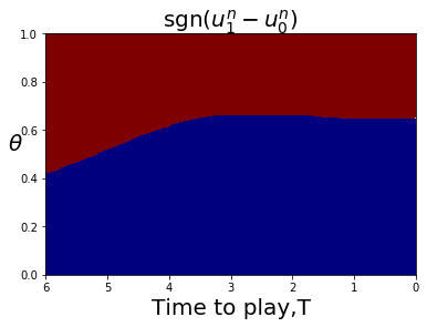 Figure 1
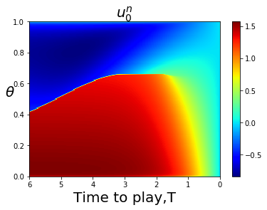 Figure 2
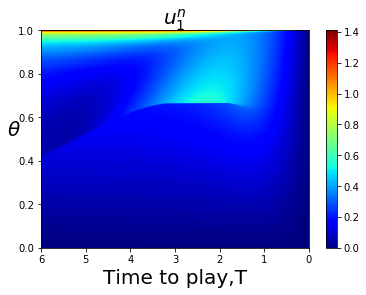 Figure 3
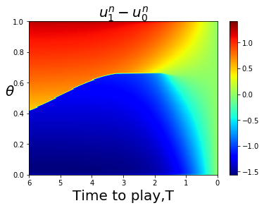 Figure 4
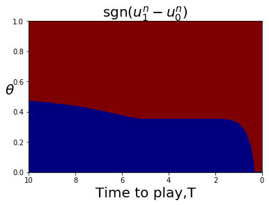 Figure 5
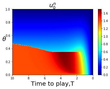 Figure 6
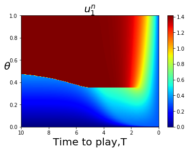 Figure 7
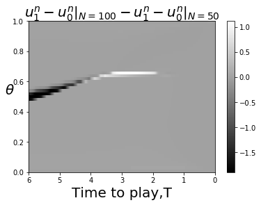 Figure 8
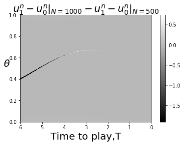 Figure 9
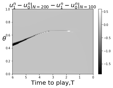 Figure 10
 Figure 11
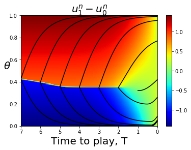 Figure 12
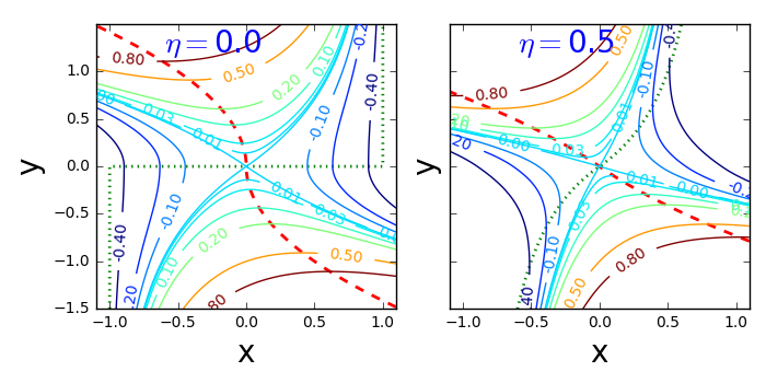 Figure 13
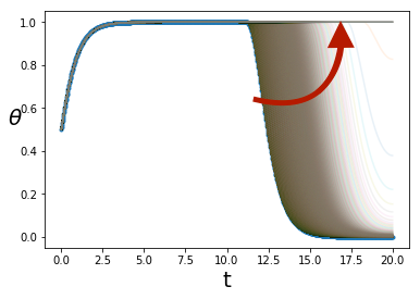 Figure 14
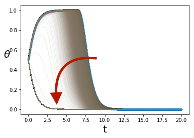 Figure 15
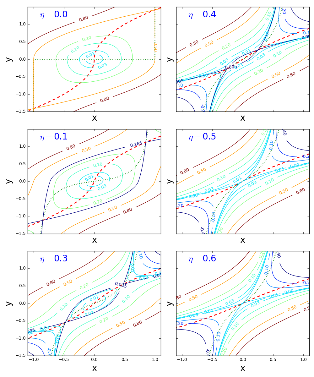 Figure 16
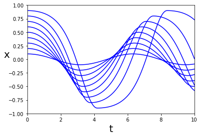 Figure 17
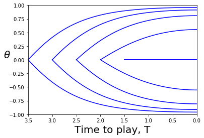 Figure 18
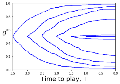 Figure 19
Peer Reviews
No public reviews on file for this paper yet. If you reviewed it on a platform where reviews are public (OpenReview, ICLR, NeurIPS, ICML), you can paste yours below so the community can read it here.
Videos
No videos yet. Explain this paper in a talk, walkthrough, or lecture? Add one.
On non-unique solutions in mean field games
Bruce Hajek and Michael Livesay
Department of Electrical and Computer Engineering and Coordinated Science Laboratory
University of Illinois, Urbana, IL 61801, USA
Email: {b-hajek, mlivesa2}@illinois.edu
Abstract
The theory of mean field games is a tool to understand noncooperative dynamic stochastic games with a large number of players. Much of the theory has evolved under conditions ensuring uniqueness of the mean field game Nash equilibrium. However, in some situations, typically involving symmetry breaking, non-uniqueness of solutions is an essential feature. To investigate the nature of non-unique solutions, this paper focuses on the technically simple setting where players have one of two states, with continuous time dynamics, and the game is symmetric in the players, and players are restricted to using Markov strategies. All the mean field game Nash equilibria are identified for a symmetric follow the crowd game. Such equilibria correspond to symmetric -Nash Markov equilibria for players with converging to zero as goes to infinity.
In contrast to the mean field game, there is a unique Nash equilibrium for finite It is shown that fluid limits arising from the Nash equilibria for finite as goes to infinity are mean field game Nash equilibria, and evidence is given supporting the conjecture that such limits, among all mean field game Nash equilibria, are the ones that are stable fixed points of the mean field best response mapping.
I Introduction and related work
The theory of mean field games was initiated independently by Huang, Caines, and Malhamé [4] and Lasry and Lions [5]. The setting of Huang et al. is linear quadratic Gaussian (LQG) control and the setting of Lasry and Lions is continuous state Markov diffusion processes. The work of Gomes, Mohr, and Souza [3] translates much of the theory of [5] into the context of continuous time finite state Markov processes. The LQG and finite state settings are technically simpler than the setting of continuous state Markov processes. All three of these works impose assumptions implying uniqueness of solutions to the mean field game equations.
The notion of Markov perfect equilibrium was introduced in [6]. It is basically a Nash equilibrium in a controlled Markovian dynamics framework, such that each player can use a strategy that selects control actions based on the current states of all players. In particular, the constraint on strategies for Markov perfect equilibria rules out trigger strategies such that some player can be punished for past actions. Given a game and , a strategy profile is defined to be an -equilibrium (or Nash equilibrium) if it is not possible for any player to gain more than in expected payoff by unilaterally deviating from his/her strategy.
The paper [4] establishes -Nash equilibrium properties for strategy profiles consisting of the decentralized individual control laws that result as responses to the collective mass trajectory. Condition H1 of [4] is a key to guaranteeing uniqueness of the mean field equations, In particular, for the other parameters fixed, the value of in the term for control cost, , should not be too small. In essence, condition H1 restricts the level of coupling among the players. The mean field game (MFG) equations are expressed as a fixed point of an operator in [4]. Proposition 4.5 of [4] states that the fixed point for is globally attracting under condition H1 in the paper. Section VI of [4] illustrates a cost gap between individual and global based controls. This is an example of the fact that the social welfare at a Nash equilibrium in game theory does not need to equal the maximum social welfare achievable if the players were to cooperate.
The paper [3] studies the continuous-time, finite state version of mean field game theory. Assumption 3, p. 110, gives a monotonicity condition that ensures uniqueness of solutions to the mean field game equations. Proposition 4 of [3], on the existence of a mean field game Nash equilibrium is proved by using Brouwer’s fixed point theorem applied to the map which is analogous to the map of [4]. The domain of is the set of uniformly Lipschitz continuous functions on the interval
In contrast, multiple solutions of the mean field equations naturally arise in [10], where synchronization of coupled oscillators requires solutions that depart from the incoherence solution. The setup is similar to the discrete-state setting we consider in that it is in continuous time, the players are coupled through their running costs, and players can take actions depending on their own states and on the states of the other players. But the setup in [10] is different in that the state space is continuous – specifically it is the unit circle, and the focus is on infinite horizon average cost. The running cost for player , is join the crowd type; it is smaller if the states are closer together. It is similar to flocking of birds or synchronization of fireflies. The separate Brownian motions of different players tend to make them drift apart, and it requires cost for them to try to stick together. If the coefficient for the cost is large enough it is not worth the players trying to stick close together, and for the MFG limit they will stay uniformly distributed over the circle (i.e. the incoherence solution). As crosses below some critical value the incoherence solution still exists but it becomes unstable and additional solutions appear. We find an equivalent phenomena for the simpler discrete state model in this paper. In addition, our setting is considerably simpler than that of [10], allowing us to examine the stability of the mean field map for a finite time horizon.
Some related papers with discrete state models The paper [9] introduces the notion of oblivious equilibrium and compares it to the stronger equilibrium notion of Markov perfect equilibrium. In a Markov perfect equilibrium, the actions of any player can depend on the current states of all players. In contrast, for an oblivious equilibrium, the actions of any player can depend only on the state of the player itself. This limits the abilities of players to react to fluctuations in population dynamics for a finite number of players. However, in the mean field limit, the population dynamics becomes deterministic, in which case the difference between the two equilibrium concepts diminishes in the large number of players limit. That is the notion explored in [9]. An approximation theory of [9] shows that an oblivious equilibrium under certain technical conditions can be approximated by a Markov perfect equilibrium, while the converse direction is not necessarily true. The setting of [9] is discrete time throughout.
Papers [1] and [8] discuss MFG for discrete state Markov processes. Paper [8] considers a so-called Markov decision evolutionary game. It is similar to the classical evolutionary dynamics setting, but in contrast to the classical setting, players have both a type (that doesn’t change) and an internal state (that evolves in a Markov fashion). The number of players involved in an event at a discrete time point is stochastically bounded, so as the number of players converges to infinity, time is sped up and a continuous time limit results. A mean field limit for fixed Markov policies exists by a Kurtz type theorem. The setting of [1] is also a discrete state Markov process for each player, The models of both [1] and [8] assume the players use so-called stationary policies, such that the action of a player depends on the type of the player and internal state of the player, but not on the states of other players. Thus, the equilibrium concept is oblivious equilibrium.
II Problem formulation
The model we adopt is almost a special case of the model of [4]. We consider players with each having state space The state of a given player evolves as a controlled Markov process with predictable control , such that the jump probabilities of the state process are given by
[TABLE]
for The parameter represents a background jump rate, so if then the process has minimum jump rate The background jumping is similar in spirit to the Brownian motions that work against coherence of the coupled oscillators in [10]. The objective function of the reference player is to select to solve
[TABLE]
where is the fraction of other players in state 0 at time The running costs are assumed to have the form such that the residence costs per unit time, and , and terminal costs, are all bounded, and uniformly Lipschitz continuous in
Hamilton Jacobi Bellman (HJB) equation for player system
A state feedback control for a given player is a nonnegative function such that represents the current state of the player, represents the number of other player in state 0, and Suppose the reference player uses a state feedback control , and the other players use state feedback control Then forms a controlled Markov process on where represents the state of the reference player and represents the number of other players in state 0. The transition rates are as follows:111If then itself is one of the “other players” for player
[TABLE]
Denote the cost-to-go function for the reference player by The HJB equations for it are:
[TABLE]
where the corresponding control policy is
[TABLE]
The HJB equations (1)-(3) can be viewed in two different ways.
- •
For policy of the other players fixed, (1) - (3) determine the best response policy for the reference player. i.e.
- •
To find a symmetric Nash equilibrium, replace and by in the definition of and (1)- (3). This yields a dimensional ode with terminal boundary condition and Lipschitz continuous right hand side that uniquely determines the functions and, hence also, the feedback control law The strategy profile such that all players use is a Markov perfect Nash equilibrium, because is determined backwards from the terminal condition yielding a best response for any interval of the form Moreover, the Markov perfect equilibrium is the unique Nash equilibrium among all Markov type (i.e. state feedback) strategy profiles, because the similar HJB equations for a more detailed model description with state space still has a unique solution and it is necessarily invariant under permutation of the players.
Mean field game equilibria and map
A mean field game Nash equilibrium for the finite horizon problem with initial value is any solution to the following equations.222Note the double use of notation “” We write for associated with mean field game solutions and for associated with the player Markov perfect equilibrium.
[TABLE]
Note that the boundary conditions (6) include both initial and terminal values. The mean field equations (4)-(6) can be written as a fixed point equation, , where maps a collective mass trajectory to another trajectory. It is determined by first computing the decentralized individual control laws for the players. Then by the uniform law of large numbers (see Appendix B), if each of the players follows the same decentralized individual control law, their state processes will be independent and the empirical average of such processes will converge to an expected that is the output collective mass trajectory. More concretely, is defined as follows. First, cost-to-go functions are determined by the HJB terminal value problem for a single player, in response to the collective mass trajectory
[TABLE]
Then the probability a single player using the decentralized state-feedback control is in state [math] at time , is determined by the initial value problem (Kolmogorov forward equation):
[TABLE]
Motivated by the law of large numbers, is defined to be the new collective mass trajectory, i.e.
The mean field game equations (4) and (5), with the addition of an average cost per unit time term on the right-hand side of (5) correspond to an infinite horizon game for average cost per unit time. (See [3], Section 2.12, p. 117.) In that case the value functions represent realative cost to go. The boundary conditions (6) are replaced by the condition that be constant in time or be periodic.
Fluid limits of Markov perfect equilibrium
As noted in the introduction, there can be multiple mean field game Nash equilibria, even for a finite horizon problem with given boundary conditions. A mean field game Nash equilibrium yields a decentralized player strategy For finite , the strategy profile such that every player uses is easily seen to be an -Nash equilibria such that as (See Appendix B.)
However, for finite there is a unique Markov perfect Nash equilibrium strategy profile, so for a given initial condition, the distribution of the finite system is uniquely determined. It is natural, therefore, to single out collective mass trajectories that arise as limits of the mass trajectories for Markov perfect equilibria.
Definition II.1**.**
Let denote the number of players in state 0 at time under the unique symmetric Markov perfect equilibrium for the player game, and for some initial condition depending on Then is a fluid limit Markov perfect trajectory (FLMP trajectory) if for some sequence of initial states with the following holds for any ,
[TABLE]
Proposition 1**.**
Suppose An FLMP trajectory is a mean field game Nash equilibrium.
See Appendix A for a proof. We conjecture the proposition is also true for but a change of probability measure argument in the proof breaks down if Proposition 1 raises the question of how to identify which mean field Nash equilibria are FLMP trajectories.
Contributions of the paper
Proposition 1 is new and its proof extends to the general setting of [3]. It shows that the search for FLMP trajectories can be limited to the mean field game Nash equilibria. The next contribution of this paper is to identify all of the MFG equilibria for a natural special case of the two state model called follow the crowd. This model is analogous to the model of synchronization of oscillators game [10], but considerably simpler, so we can identify the finite horizon solutions as well as the infinite horizon ones. The third contribution is to offer the following conjecture, and give evidence for it:
Conjecture 1**.**
The FLMP trajectories are the stable fixed points of the MFG mapping
A similar type of conjecture is implicit in [10] based on a notion of stability for constant, long-term average cost infinite horizon solutions, called linear asymptotic stability. The paper [10] identifies the critical cost threshold at which the incoherence solution becomes unstable. In addition to giving evidence for Conjecture 1 in the setting of finite horizon games, we also show that the results of [10] for constant, long-term average cost infinite horizon solutions, carry over to the setting of two state Markov processes. For the infinite horizon framework, we show asymptotic stability of certain fixed points for the nonlinear dynamics in Section III-C, and Appendix D gives an analysis based on the notion of linear asymptotic stability introduced in [10]. Additional results are given in the appendix of this paper, including, for contrast, a similar analysis for an avoid the crowd model with unique mean field game solutions, and a description of a partial differential equation (PDE) (given for more general model in [3]) that can be considered to be an extension of the notion of mean field game.
III MFG equilibria for follow the crowd
The follow the crowd model corresponds to the following cost per time spent in state :
[TABLE]
In particular, if (more than half of the other players in state 0), then state 0 has smaller cost per unit time than state 1.
Letting the mean field equations (4)- (6) can be written as:
[TABLE]
with the boundary conditions and Once a solution to (12) is found for the finite horizon problem over , a corresponding solution to the mean field game equations can be found by simply integrating (4)- (5) because the righthand sides of (4)- (5) are determined by
A useful fact is that the equations (12) form a Hamiltonian system, for the Hamiltonian function :
[TABLE]
In other words, (12) has the form and where and represent partial derivatives of Consequently, the value of is constant along the solutions of (12), because so the trajectories trace out level contours of This model is a special case of potential mean field games defined in [3], Section 5, for which Hamiltonians exist.
Contour maps of are shown in Fig. 1 for various values of
For small values of the quadratic terms in dominate the cubic term, and for , constant gives elliptical orbits of in the clockwise direction.
III-A Finite time horizon mean MFG solutions
For the finite horizon mean field game with zero terminal cost (i.e. terminal boundary condition ), and initial state , correspond to paths that begin on the axis (so the initial condition is satisfied) and end on the axis. One solution is for Let denote the angle of from the positive axis. The angular velocity of is given by
[TABLE]
It is negative along the axis, indicating clockwise motion. If then along the line , indicating that is never reached. Thus, if , the trajectory is the only MFG equilibrium.
If then for in a neighborhood of the origin, indicating clockwise movement. Moreover, for fixed, is an increasing function of the distance of to the origin (decreasing angular speed because angular velocity is negative). Thus, the time for to traverse a contour across the first quadrant is increasing in for As the dynamics is given, to first order, by the MFG linearized about , given by
[TABLE]
with solution of the form (setting and ):
[TABLE]
The time it takes the linear system to traverse the first quadrant is Hence, as the traversal time for the quadrant converges to Thus, for and is the unique solution to the MFG. For there is one more solution that remains in, and traverses, the first quadrant, and the negative of that solution remains in, and traverses, the third quadrant. For large enough there are solutions that traverse contours of through three quadrants, five quadrants, and so on. A similar radial velocity analysis for the pair (see Appendix C) establishes that the entire periods of the dynamical system are increasing with amplitude, as illustrated in Fig. 2. Since the dynamics is symmetric under rotation by we conclude that for any odd number , starting on the positive axis, the time required to rotate through quadrants is increasing in the initial condition Therefore, as increases from 0, the number of solutions starts at one and jumps up by two when crosses times of the form for Equivalently, the number of solutions is
III-B Infinite horizon constant or periodic MFG solutions
The equilibrium points of the dynamics (12) are the critical points of the Hamiltonian function (i.e. ), and are given as follows. If is an equilibrium point and there are also exactly two nonzero equilibrium points, given by , where
[TABLE]
If is the unique equilibrium point.
Regarding infinite horizon periodic solutions, examination of and the equations for angular velocity, (14) and similar equation for angle of , lead to the following conclusions. If there is a two-dimensional family of periodic solutions that can be indexed by the peak amplitude of (ranges over and phase. The period of the solutions increases continuously over as the peak amplitude of increases over . If there are no periodic solutions of (12).
III-C *Infinite horizon convergent transient MFG solutions, and the asymptotically stable
constant solutions*
Consider the initial value problem over with some initial condition and dynamics (12). First, suppose For any initial condition such that , one of four cases holds: is periodic with a positive period, converges to , converges to , or exits in finite time. The following categorize the convergent solutions such that remains in
- •
For any initial value of , there exist two corresponding initial values of such that the solution of the initial value problem satisfies (i) for all and (ii) the solution converges to a limit as For the smaller value of the limit is and for the larger value of the limit is The value of the larger for example is such that the contour of through contains
- •
For an initial value there exists a unique value of such that the solution of the initial value problem satisfies for all That solution converges to as
- •
Similarly, for an initial value there exists a unique value of such that the solution of the initial value problem satisfies for all That solution converges to as
Second, suppose For any , there is a unique value of , such that the solution of the initial value problem for (12) satisfies for all Furthermore, has the same sign as , and the solution converges to as The value of is the root of (for fixed) that is closer to zero.
The above observations give a sense in which is an asymptotically stable equilibrium point of the dynamics (12) if and is an asymptotically stable equilibrium point if This sense of stability is not the usual definition of (Lyapunov) stability because we ask, for given , whether there exists an associated value of giving the desired convergence. The asymptotically stable limit points are saddlepoints of
As mentioned above, a related definition of stability, called linear asymptotic stability, is formulated in [10]. That definition and the results of [10] for it are translated to the model of this paper in Appendix D.
IV Evidence for Conjecture 1
In order to explore whether Conjecture 1 is true, it is natural to explore two sides of the question. One side is to identify the FLMP trajectories. Numerically that can be done by solving the dimensional HJB equation for the system with players to find the strategy players use for the Markov perfect equilibrium with players, and then either simulating the corresponding occupancy process through Monte Carlo simulation of players independently using that policy, or solving the Kolmogorov forward equations to find the marginal distribution, mean and variance of the number of players in state 0 vs. time.
The other side is to identify the stable fixed points of Two ways to explore which fixed points of are stable are to either numerically investigate the orbit trajectories as is repeatedly applied to some initial trajectory, or to examine the linearization of about a fixed point–this is the Gateaux derivative and it can be expressed as an integral operator. The eigenvalues can be computed numerically, and in rare cases, analytically. By abuse of notation, we use to denote the mean field map as a mapping obtained by the change of coordinates
Numerical identification of FLMP trajectories
For the symmetric follow the crowd model, numerical analysis strongly and consistently indicates which MFG solutions are FLMP trajectories. We find that for they coincide with the unique MFG equilibrium – namely, the (0,0) trajectory over And for there are two FLMP trajectories. Namely, the one that traverses the first quadrant in the x-y plane once, and the negative of it, which traverses the third quadrant in the x-y plane once. In particular, the solutions that wind around the origin through three or more quadrants do not appear to be FLMP solutions. See Fig. 3 for illustration.
For less symmetric examples it is less obvious where the bifurcation curve is that separates FLMP solutions that converge to a point closer to 1, or converge to a point closer to 0. The bifurcation curve often coincides with a line or curve of indifference for the player game with a large number of players, corresponding to upcrossings of zero by the mapping This is illustrated in Fig. 4.
Examination of orbits of
Recall that the fixed points of are the collective mass trajectories of mean field Nash equilibria. To numerically investigate the stability of fixed points of we generated sequences of iterates of trajectories defined by where the initial point is a perturbation of a fixed point. Figure 5 shows such sequences of iterates such that the initial trajectory is a perturbation of one of the two MFG Nash equilibria that cross zero one time, for the follow the crowd game and time horizon In both instances, the iterates converged to one of the two equilibria with no zero crossings.
However, overall we found it difficult to numerically verify that a given solution is not a stable fixed point. On one hand, some MFG solutions that we don’t expect to be stable, such as the trajectory that crosses zero once, numerically appear to be asymptotically stable for a very small basin of stability. On the other hand, we have found perturbations of MGF solutions that also numerically appear to be asymptotically stable, indicating numerical artifacts are possible.
Linearization of about
Given a fixed point , the Gateaux derivative , or the directional derivative of at in the direction is obtained by linearizing about This is particularly simple if is the zero trajectory. (Linearization about a nonzero trajectory is given in Appendix E.) In that case, the linearized MFG equations are:
[TABLE]
Given , , where and are linear operators defined as:
[TABLE]
These expressions can be combined to yield
[TABLE]
where for and for In other words, the Gateaux derivative is the integral operator with kernel
If , which is the covariance of Brownian motion, which has a well known Mercer series expansion. The eigenvalues of are with corresponding eigenfunctions for In particular, the largest eigenvalue is and if and only if where is the critical time horizon for the appearance of multiple MFG equilibria.
Here is an upper bound on the maximum eigenvalue of for The mappings and are both bounded operators in the supremum norm: with operator norm Thus, the Gateaux derivative is also a bounded operator in the supremum norm with operator bound 333A somewhat tighter bound is given by where , but the expression for is complicated. Hence, if , the linearized mapping is a contraction in the norm for all If it is a contraction if is small enough that
For we conjecture the largest eigenvalue of is greater than one precisely when there is a nonzero MFG equilibrium, namely, when We numerically found the largest eigenvalue of the matrix approximation of the kernel, for for and near and the calculations match the conjecture well.
Appendix A Proof of Proposition 1
This section proves Proposition 1, that if FLMP trajectories are mean field game equilibria. The proof is given after some initial notation is given and two lemmas are proved. Let be an FLMP trajectory and let be a corresponding sequence of initial conditions as in the definition of FLMP trajectory. For , let denote the controlled Markov process for players resulting for initial state when all players use the unique policy for the Markov perfect equilibrium for players. Since the functions and are bounded, for fixed, the cost to go functions determined by the HJB equations (1)- (34) are uniformly bounded for all and Therefore, the policy , determined by (3), is also uniformly bounded. Select such that for all and Suppose also that is large enough that for all for any decentralized policy resulting by responding to a deterministic collective mass trajectory.
Consider the following variation of the Markov perfect equilibrium. Suppose the reference player switches from using to some other policy, such that and is continuous for all Let denote the original probability distribution for the process and let denote the probability distribution of when the reference player switches to policy
Lemma 1**.**
(Insensitivity of FLMP trajectory to one player switching policies) The following holds for any ,
[TABLE]
Lemma 2**.**
Let and be probability distributions on the same measurable space such that (i.e. is absolutely continuous with respect to ) and let denote the Radon-Nikodym derivative. Suppose for some and Let be such that Then for any event ,
Proof of Lemma 2.
By Hölder’s inequality,
[TABLE]
∎
Proof of Lemma 1 .
Since and only differ by the change in the policy for player 1, the Radon-Nikodym derivative can be written explicitly as follows. Let denote the number of jumps of the state of the reference player during Then, by standard theory of change of probability measure for point processes (Girsanov type result for point processes, see [7], Theorem 4.1 for example), and the Radon-Nikodym derivative is given by
[TABLE]
where is short for is short for and is the fixed positive background jump rate.
Note that for , the expression for the Radon-Nikodym derivative to the power can be written as a product
[TABLE]
where is a probability measure corresponding to a similar Radon-Nikodym derivative with a factor in front of the log term, and Thus, Lemma 1 thus follows from Lemma 2 with equal to the complement of the event in (22). ∎
Proof of Proposition 1.
Consider the Markov perfect equilibrium for large In view of Lemma 1, if the reference player deviates from using , the normalized process for the rest of the population still follows arbitrarily closely as Thus, an asymptotically optimal policy for the reference player to switch to is the optimal response to deterministic collective mass trajectory Furthermore, it implies converges to zero uniformly in and , where is associated with the player MP equilibrium, and is the cost-to-go for the single reference player responding to the deterministic mass trajectory It follows that all players in the game are asymptotically effectively using the same policy as the alternate policy of the reference player. (in other words, Thus, the corresponding fluid limit is the same as the mean limit for the reference player with random initial state equal to 0 with probability ∎
Appendix B The uniform law of large numbers
Theorem 7.4 of [2] is repeated here for convenience.
Proposition 2**.**
Let be a centered, stochastically continuous uniformly bounded random process whose trajectories are right continuous and have left limits. Assume for some , some nondecreasing function and for all Then in
An implication of this theorem is that if all players use the same decentralized policy (assumed to be bounded and measurable in ) and if the initial conditions satisfy for some then as the population average converges to in probability in the supremum norm, where is determined by the Kolmogorov forward equation
[TABLE]
Therefore, the following are equivalent for a trajectory :
- (a)
Let denote the optimal response policy for a single player in response to In other words, where is determined by (7)- (8). Then for any and any sequence of finite player games with , the strategy profile of all players using is an -Nash equilibrium for sufficiently large . 2. (b)
is the population trajectory of a MFG equilibrium.
Appendix C Monotonicity of period with amplitude
Consider the follow the crowd dynamics (12), rewritten here for convenience:
[TABLE]
From (12) we find for all
[TABLE]
Equivalently, writing , yields
[TABLE]
The motion (25) admits the Hamiltonian If then is convex near the origin. Letting we find
[TABLE]
Note that is increasing in for any fixed ratio of to (decreasing angular speed). Hence, the period of the periodic trajectories increases with amplitude.
Appendix D Linear asymptotic stability for symmetric follow the crowd example
A definition of linear asymptotic stability was introduced in ([10], Section IV) for a constant in time solution to the infinite horizon long term average cost mean field game. We translate that definition to our setting. Roughly speaking, linear asymptotic stability is a variation, based on linearization, of the asymptotic stability properties delineated in Section III-C.
Definition 1**.**
Suppose is an equilibrium point for the ode (12). Seeking solutions of the form , we obtain a linear initial value problem for by linearizing (12) about The point is said to be linearly asymptotically stable if for any initial perturbation there exists a unique solution to the linearized equations (with the given initial condition for , some initial condition for , and satisfying the constraint ) and, furthermore,
With the definition in place we prove the following proposition.
Proposition 3**.**
The equilibrium point is linearly asymptotically stable if and only if The equilibrium points are linearly asymptotically stable if and only if
Proof.
For an equilibrium point , we have and
[TABLE]
So the linear initial value problem for can be written as
[TABLE]
where
[TABLE]
Since (so sum of eigenvalues is zero) and where is the Hessian of :
[TABLE]
the eigenvalues of are If then the eigenvalues are real valued and one is negative. If the eigenvalues are purely imaginary. For the follow the crowd game with Hamiltonian given in 13,
[TABLE]
Consider first the zero equilibrium, in which case A=\left(\begin{array}[]{cc}-2\eta&1\\ -1&2\eta\end{array}\right). This has eigenvalues and, for , corresponding eigenvectors If then the solutions to (26) have the following form, for some constants and ,
[TABLE]
The initial condition for and the constraint are satisfied if and only if and and the resulting solution converges to zero as Hence, the system is linearly asymptotically stable if If then the two eigenvalues of are purely imaginary, nonzero, and negatives of each other, so that all nonzero solutions to (26) are periodic. If all solutions have of the form So, combining the observations for and , we conclude that for there are no nonzero solutions satisfying the constraint. So for the zero equilibrium is not linearly asymptotically stable.
Now consider the equilibrium point and suppose Then, since we find that Therefore, by the analysis for the zero equilibrium point with replaced by , we see that again has two real-valued eigenvalues of opposite sign, so the system is linearly asymptotically stable. ∎
Note that the eigenvalues for the equilibrium point have qualitatively the same graph as in Figure 2(b) of [10], with and replaced by and
Remark 1**.**
Proposition 3 illustrates the notion of linear asymptotic stability for equilibrium points of the infinite horizon average cost mean field game, introduced in [10]. The two state Markov control problem we have considered is considerably simpler than the coupled oscillator problem considered in [10], so, as explained in Section III-C, we could observe asymptotic stability properties of equilibrium points directly, rather than considering the linearized dynamics.
Appendix E Kernel for Gateaux derivative of for nonzero
We give an expression for the kernel of the Gateaux derivative along a nonzero trajectory in case for follow the crowd cost function. Given , is found by first finding :
[TABLE]
and then
[TABLE]
Fix and sufficiently small. Suppose . Let , and Let be the solution to (27) with the respectively. Then, linearizing the equations for and yields
[TABLE]
so that
[TABLE]
and the kernel of is thus given by
[TABLE]
If over then yielding:
[TABLE]
Appendix F Avoid the crowd cost function
In contrast to the follow the crowd game focused on in this paper, the MFG equilibrium for the avoid the crowd game of this section has a unique solution. Suppose the cost per time spent in state is
[TABLE]
where is the fraction of other players in state 0.
The reduced dimension MFG equations become
[TABLE]
with associated Hamiltonian
[TABLE]
Contour maps of are shown in Fig. 6 for two values of
We observe that is the unique critical point of and for any there exists a unique value of such that the solution of the initial value problem with dynamics (31) over is such that for all Furthermore, such solution converges to . Also, and the unique equilibrium point of the infinite horizon average cost MFG is linearly asymptotically stable.
Appendix G On the difference of cost to go for players
Recall that using defined by yielded a reduction from three to two dimensions in the MFG equilibrium equations. Let us see if a similar reduction occurs for the Nash equilibrium equations for the player game. For convenience we restate the HJB cost-to-go equations (1) and (3) for the reference player in the player game:
[TABLE]
where the corresponding control policy is
[TABLE]
Suppose all players use policy , so in the definition of Let and Using the facts
[TABLE]
in (33) yields
[TABLE]
The RHS is not a function of alone. However, using and yields the approximation:
[TABLE]
Appendix H The MFG partial differential equation
An interpretation of a mean field game Nash equilibrium is that at each time , is the cost to go for a reference player in state , given that the fraction of players in state 0 is That picture can be embedded into a larger picture. Bt taking a limit of the HJB equations for players as we can derive a PDE for such that is the cost-to-go for a reference player in state given that the fraction of players in state 0 is for any This idea is described in [3] (see Proposition 8) and is attributed there to P. Lions. For simplicity, we derive the PDE for the avoid the crowd game and use the equations derived in Section G. We use notation instead of and instead of
Equations (36)-(37) suggest the following PDE, where now is treated as a continuous variable over rather than as an integer variable.
[TABLE]
Note that if we let be defined by the following initial value problem
[TABLE]
then by the chain rule and the PDE (38),
[TABLE]
Note that if we set and and consider the join-the-crowd cost function (so ), then (40) and (41) are equivalent to the MFG equations (12). This calculation is an instance of Proposition 8 of [3]. Figure 8 gives numerical evidence that , with normalized to , converges as Presumably the limit is the solution of the PDE.
The PDE (38)- (39) is a first order hyperbolic type. Equation (40) defines a characteristic curve for the PDE, which is why the PDE along the curve reduces to an ODE. The fact there are multiple MFG solutions indicates that solutions of the PDE are also not unique. The problem of identifying which MFG Nash equilibria are FLMP trajectories therefore can be extended to the problem of determining which solutions of the PDE are limits of the scaled cost-to-go functions
The reference list from the paper itself. Each links out to its DOI / PubMed record.
- 1[1] E. Altman, K. Avrachenkov, N. Bonneau, M. Debbah, R. El-Azouzi, and D. S. Menasche. Constrained cost-coupled stochastic games with independent state processes”. Oper. Res. Lett. , 36(2):160–164, 2008.
- 2[2] E. Giné and J. Zinn. Some limit theorems for empirical processes. The Annals of Probability , 12:929–989, 1984.
- 3[3] Diogo A Gomes, Joana Mohr, and Rafael Rigão Souza. Continuous time finite state mean field games. Applied Mathematics & Optimization , 68(1):99–143, 2013.
- 4[4] Minyi Huang, Peter E Caines, and Roland P Malhamé. Large-population cost-coupled LQG problems with nonuniform agents: Individual-mass behavior and decentralized ε 𝜀 \varepsilon -Nash equilibria. IEEE Transactions on Automatic Control , 52(9):1560–1571, 2007.
- 5[5] J.-M. Lasry and P.-L. Lions. Mean field games. Japanese Journal of Mathematics , 2(1):229–260, 2007.
- 6[6] Maskin and Tirole. A theory of dynamic oligopoly, I and II. Econometrica , 56:549–570, 1984.
- 7[7] Jan H. Van Schuppen and Eugene Wong. Transformation of local martingales under a change of law. The Annals of Probability , 2(5):879–888, 1974.
- 8[8] H. Tembine, J.-Y. Le Boudec, R. El-Azouzi, and E. Altman. Mean field asymptotics of markov decision evolutionary games and teams. In Proc. 1st ICST Int. Conf. Game Theory for Netw , pages 140–150, 2009.