Adiabatic quantum dynamics under decoherence in a controllable trapped-ion setup
Chang-Kang Hu, Alan C. Santos, Jin-Ming Cui, Yun-Feng Huang, Marcelo, S. Sarandy, Chuan-Feng Li, Guang-Can Guo

TL;DR
This paper investigates how adiabatic quantum processes behave under decoherence in a controllable trapped-ion setup, combining theoretical analysis and experimental implementation to understand robustness and optimize outcomes.
Contribution
It provides the first combined theoretical and experimental study of adiabatic quantum dynamics under decoherence in a trapped-ion system, highlighting conditions for robustness and practical quantum algorithm execution.
Findings
Decoherence can sometimes promote adiabaticity in open quantum systems.
Optimal time windows exist for successful adiabatic quantum computation under decoherence.
Experimental validation using a single trapped Ytterbium ion demonstrates controllable decoherence effects.
Abstract
Suppressing undesired nonunitary effects is a major challenge in quantum computation and quantum control. In this work, by considering the adiabatic dynamics in presence of a surrounding environment, we theoretically and experimentally analyze the robustness of adiabaticity in open quantum systems. More specifically, by considering a decohering scenario, we exploit the validity conditions of the adiabatic approximation as well as its sensitiveness to the resonance situation, which typically harm adiabaticity in closed systems. As an illustration, we implement an oscillating Landau-Zener Hamiltonian, which shows that decoherence may drive the resonant system with high fidelities to the adiabatic behavior of open systems. Moreover we also implement the adiabatic quantum algorithm for the Deutsch problem, where a distinction is established between the open system adiabatic density operator…
Click any figure to enlarge with its caption.
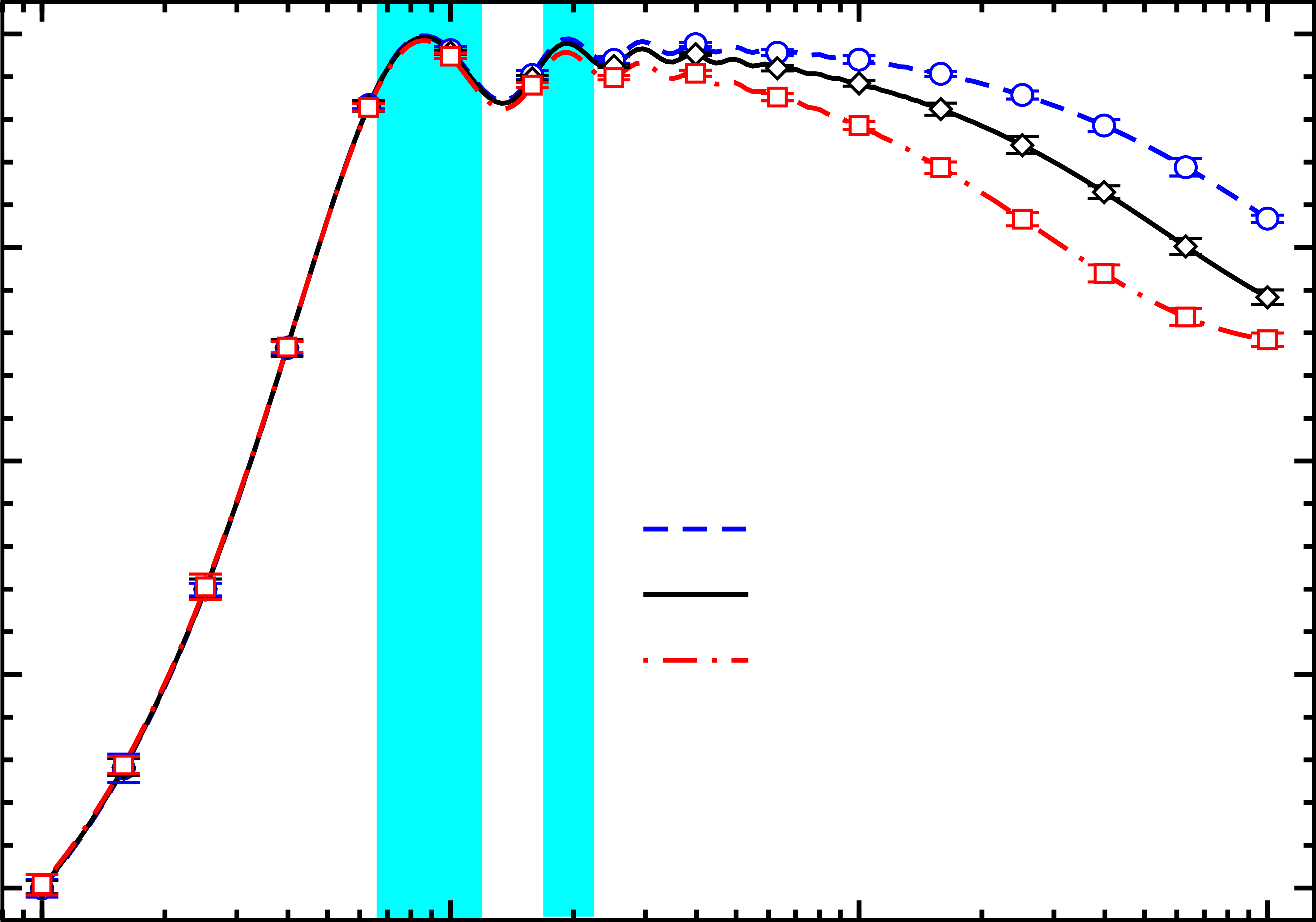 Figure 1
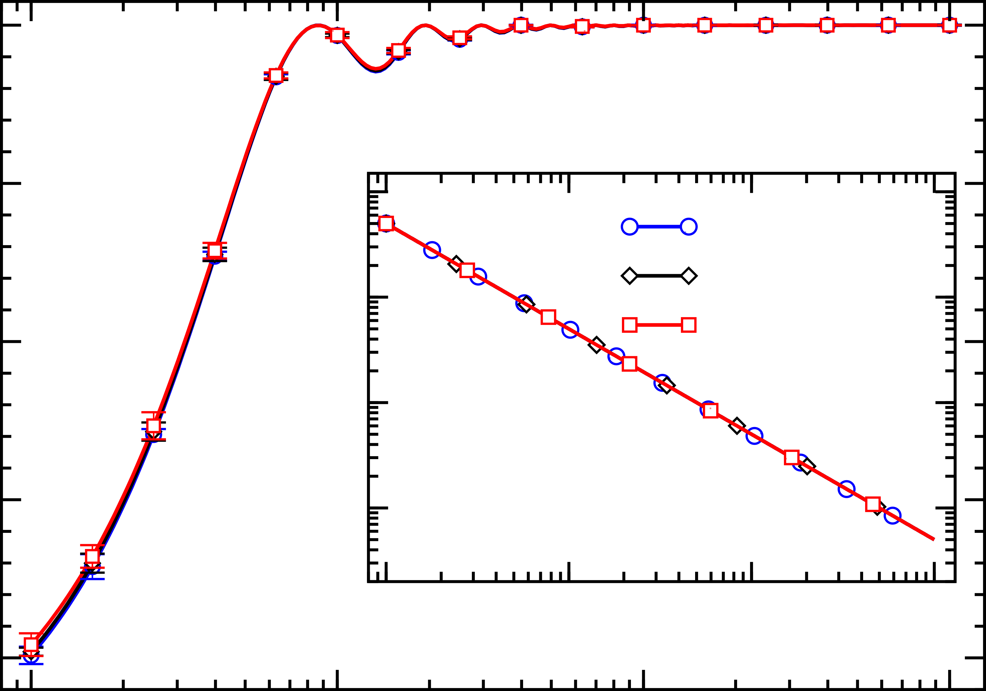 Figure 2
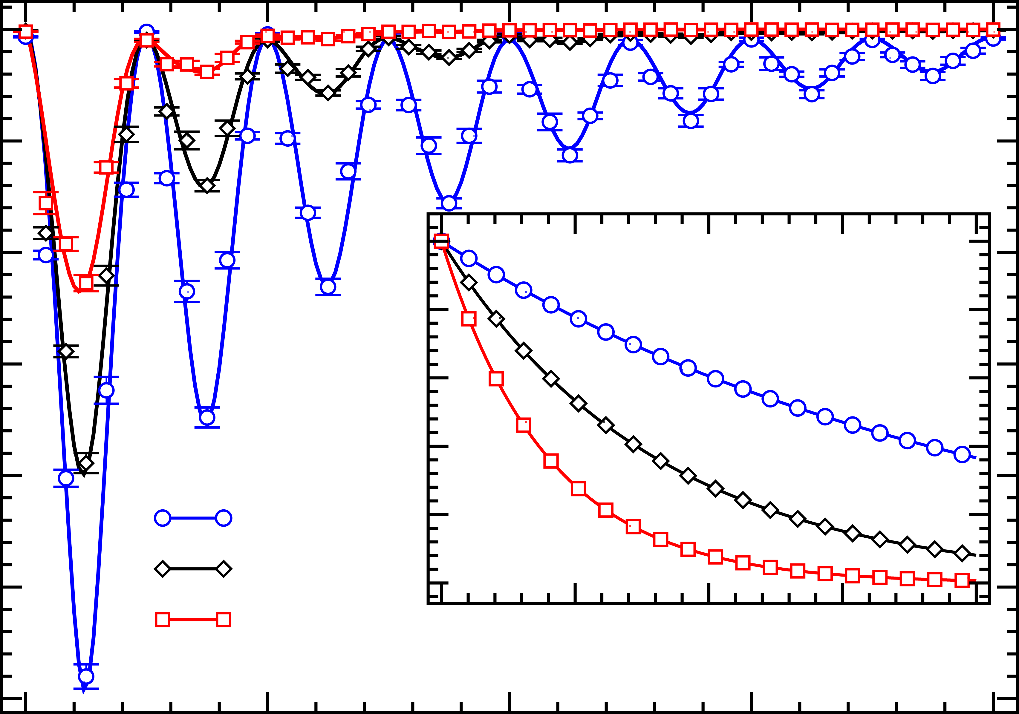 Figure 3
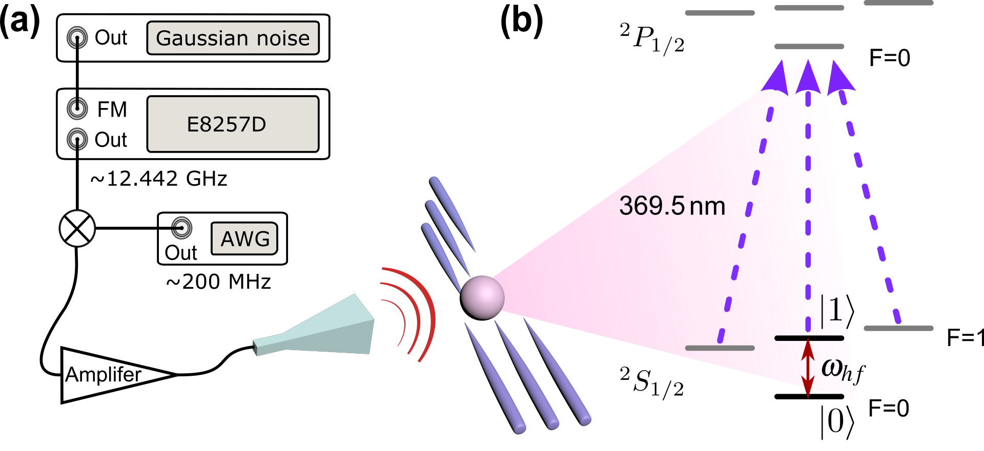 Figure 4
Peer Reviews
No public reviews on file for this paper yet. If you reviewed it on a platform where reviews are public (OpenReview, ICLR, NeurIPS, ICML), you can paste yours below so the community can read it here.
Videos
No videos yet. Explain this paper in a talk, walkthrough, or lecture? Add one.
Adiabatic quantum dynamics under decoherence in a controllable trapped-ion setup
Chang-Kang Hu
CAS Key Laboratory of Quantum Information, University of Science and Technology of China, Hefei 230026, People’s Republic of China
CAS Center For Excellence in Quantum Information and Quantum Physics, University of Science and Technology of China, Hefei 230026, People’s Republic of China
Alan C. Santos
Instituto de Física, Universidade Federal Fluminense, Av. Gal. Milton Tavares de Souza s/n, Gragoatá, 24210-346 Niterói, Rio de Janeiro, Brazil
Jin-Ming Cui
CAS Key Laboratory of Quantum Information, University of Science and Technology of China, Hefei 230026, People’s Republic of China
CAS Center For Excellence in Quantum Information and Quantum Physics, University of Science and Technology of China, Hefei 230026, People’s Republic of China
Yun-Feng Huang
CAS Key Laboratory of Quantum Information, University of Science and Technology of China, Hefei 230026, People’s Republic of China
CAS Center For Excellence in Quantum Information and Quantum Physics, University of Science and Technology of China, Hefei 230026, People’s Republic of China
Marcelo S. Sarandy
Instituto de Física, Universidade Federal Fluminense, Av. Gal. Milton Tavares de Souza s/n, Gragoatá, 24210-346 Niterói, Rio de Janeiro, Brazil
Chuan-Feng Li
CAS Key Laboratory of Quantum Information, University of Science and Technology of China, Hefei 230026, People’s Republic of China
CAS Center For Excellence in Quantum Information and Quantum Physics, University of Science and Technology of China, Hefei 230026, People’s Republic of China
Guang-Can Guo
CAS Key Laboratory of Quantum Information, University of Science and Technology of China, Hefei 230026, People’s Republic of China
CAS Center For Excellence in Quantum Information and Quantum Physics, University of Science and Technology of China, Hefei 230026, People’s Republic of China
Abstract
Suppressing undesired nonunitary effects is a major challenge in quantum computation and quantum control. In this work, by considering the adiabatic dynamics in presence of a surrounding environment, we theoretically and experimentally analyze the robustness of adiabaticity in open quantum systems. More specifically, by considering a decohering scenario, we exploit the validity conditions of the adiabatic approximation as well as its sensitiveness to the resonance situation, which typically harm adiabaticity in closed systems. As an illustration, we implement an oscillating Landau-Zener Hamiltonian, which shows that decoherence may drive the resonant system with high fidelities to the adiabatic behavior of open systems. Moreover we also implement the adiabatic quantum algorithm for the Deutsch problem, where a distinction is established between the open system adiabatic density operator and the target pure state expected in the computation process. Preferred time windows for obtaining the desired outcomes are then analyzed. We experimentally realize these systems through a single trapped Ytterbium ion 171Yb+, where the ion hyperfine energy levels are used as degrees of freedom of a two-level system, with both driven field and decohering strength efficiently controllable.
I Introduction
The impossibility of decoupling an open quantum system from its surrounding environment has motivated the development of methods to minimize the harmful nonunitary effects on a quantum evolution Petruccione:Book . In some specific cases (see, e.g., Ref. Childs:01 ), such effects can be smoothened for slowly driven Hamiltonians, which are governed by the adiabatic theorem Born:28 ; Messiah:Book ; Kato:50 . Adiabatic evolutions have been extensively used in a number of applications, such as geometric phases Berry:84 ; Wilczek:84 , quantum computation Farhi:01 ; Bacon:09 ; Barends:16 ; Johnson:11 ; Hen:15 , quantum thermodynamics Alicki:79 ; Kosloff:84 ; Quan:07 ; Geva:92 ; Henrich:07 , quantum game theory dePonte:18 , among others Vitanov:99 ; Amniat:12 ; Chu:08 . For closed systems, adiabaticity is associated with a decoupled dynamics of eigenspaces corresponding to distinct energy eigenvalues in the spectrum of a quantum Hamiltonian. In particular, assuming no level crossings in the energy spectrum along the evolution, if a quantum state is prepared in an instantaneous non-degenerate eigenstate of a sufficiently slowly varying Hamiltonian at an initial time then it will evolve to the corresponding instantaneous eigenstate at later times. Remarkably, this picture has been challenged for quantum systems driven by highly oscillating fields under resonant conditions Marzlin:04 , which may imply the failure of the expected adiabatic behavior. In particular, this issue has been experimentally investigated in a nuclear magnetic resonance setup Suter:08 , where it has been shown that many previously introduced quantitative adiabatic conditions Tong:07 ; Jianda-Wu:08 ; Ambainis:04 may fail at resonance. As an alternative to deal with this problem, a validation mechanism for adiabaticity has been recently introduced and experimentally realized via ion traps Hu-18-b . In this approach, adiabatic conditions may be consistently verified by adopting non-inertial reference frames.
Concerning open quantum systems, a generalization of the adiabatic theorem can be directly achieved for nonunitary evolution under time-local master equations governed by a Lindbladian super-operator . In this case, as originally derived in Ref. Sarandy:05-1 , open system adiabaticity can be defined by replacing the concept of decoupled evolution of eigenspaces of a Hamiltonian for the decoupled evolution of Jordan blocks Horn:Book of a Lindbladian . The open system adiabatic behavior reduces to the closed case as decoherence vanishes and implies, in general, in a finite optimal time for Jordan block decoupling, since there is a competition between the adiabatic time scale (requiring slow evolution) and the relaxation time scale (requiring fast evolution) Sarandy:05-2 . This is rather different from the traditional closed system case, where adiabaticity is favored by long evolution times, being exact at the infinite time limit. In a related approach, Refs. Venuti:16 ; Venuti:17 consider adiabatic paths that exactly hold in the infinite time limit for open quantum systems initially prepared in the steady state of at , which is associated with the Lindblad Jordan block with zero eigenvalue.
In this work, we introduce a realization of the open system adiabatic theorem considering quantum states initially prepared in general one-dimensional Jordan blocks of , investigating the adiabatic behavior in a decohering environment both at resonance and off-resonance. The experimental setup is based on a hyperfine quantum bit (qubit) built upon a single trapped Ytterbium ion 171Yb+, where the ion hyperfine energy levels are used as degrees of freedom of a two-level system (see, e.g., Refs. Hu:18 ; Hu-18-b ). As illustrations of our approach, we implement an oscillating Landau-Zener Hamiltonian, specifically introduced to investigate the effects of resonance, and the adiabatic quantum algorithm for the Deutsch problem, where fidelities can be interpreted in terms of computation outcomes. As expected in a nonunitary evolution, we will emphasize a distinction between the open system (mixed) adiabatic density operator and the target pure state expected as the result of the computation process. As we will show, since an open system typically evolves to a mixed state, the adiabatic density operator will usually provide (at most) an approximation of the target desired state. This approximation will occur at specific finite time windows, which must be taken into account to ensure the success of the algorithm. Moreover, for both cases, we provide a class of density operators for which the open system adiabaticity occurs at the infinite time limit, circumventing the usual competition between the adiabatic and relaxation time scales. As a by-product, this is shown to simplify the general quantitative condition obtained Ref. Sarandy:05-1 for a class of initial quantum states.
II Adiabatic approximation for open quantum systems
Let us consider a discrete -dimensional open quantum system described by a density operator . The nonunitary evolution of the system is assumed to be driven by a time-local master equation given by
[TABLE]
where is the Lindbladian operator and the subscript denotes that may be time-dependent. As in Ref. Sarandy:05-1 , the open system adiabatic dynamics is conveniently derived by adopting the superoperator formalism Alicki:Book1 . In this formalism, Eq. (1) can be rewritten as
[TABLE]
where is the -dimensional coherence vector and is a -dimensional matrix. The components of the vector are obtained from and the elements of are written as , where is a matrix basis obeying and 111From these definitions, one identifies the inner product between two elements and as .. Here, we will consider the particular case a superoperator whose Jordan decomposition Horn:Book admits one-dimensional Jordan blocks only, which will be individually associated with distinct non-crossing time-dependent eigenvalues . As provided in Appendix A, the adiabatic behavior will follow from the adiabatic quantum condition (AQC)
[TABLE]
where is the adiabatic parameter, reading
[TABLE]
with and denoting the right and left eigenstates of with eigenvalues , respectively, and representing the real part of . Eq. (3) ensures decoupled evolution of Jordan-Lindblad eigenspaces Sarandy:05-1 . The energy scale takes into account both the Hamiltonian spectrum and the decohering rates. The coherence vector for an arbitrary time can be expanded as , where are complex functions of time associated with the right eigenbasis of . It is important to highlight that, unlike the closed system case Sarandy:04 ; Amin:09 ; Tong:07 ; Jianda-Wu:08 ; Ambainis:04 , the adiabatic parameter in Eq. (4) is such that due to the presence of the factor . This means that, if we have , then the dynamics of is decoupled from the coefficient , but it does not mean that is decoupled from . Moreover, the real exponential in the factor is responsible for the general finite optimal time for the adiabatic behavior in open systems Sarandy:05-1 . However, we can show that, under decoherence, adiabaticity may still occur in the infinite time limit, as it happens for closed systems, for a class of initial quantum states. Indeed, let be a Lindblad superoperator that admits one-dimensional Jordan blocks with distinct eigenvalues . Assume that the initial state of the system can be written as a superposition of two independent eigenvectors of and that there are no eigenvalue crossings in the spectrum of . Then, the adiabatic dynamics in open system is achieved for slowly-varying Lindblad superoperators , with decoupling of Jordan blocks of increasing as . See Appendix B for a detailed proof of this statement.
III Open system AQC for highly oscillating driven fields
III.1 Landau-Zener model under dephasing
In order to investigate the adiabatic behavior of open systems in a controllable experimental realization, let us consider, as our first example, the single-qubit Landau-Zener Hamiltonian, which is given by
[TABLE]
This Hamiltonian presents a resonant configuration when , as shown in Appendix C. Indeed, it can be used to illustrate the fact that, due to resonance, several quantitative adiabatic conditions designed for closed systems Sarandy:04 ; Amin:09 ; Tong:07 ; Jianda-Wu:08 ; Ambainis:04 ; Suter:08 are neither necessary nor sufficient to describe the adiabatic behavior in the model if the analysis is performed in the traditional inertial reference frame Hu-18-b . Concerning decoherence, we consider that the qubit is coupled to a dephasing reservoir evolving under a Lindblad master equation
[TABLE]
with denoting a time-independent dephasing rate. By rewriting Eq. (6) in the superoperator formalism we obtain a -dimensional superoperator whose elements are . So, we have (by adopting the basis )
[TABLE]
The system is initialized in the ground state of , which is given by . Then, the coherence initial vector is written as , where the eigenvectors of the driving super-operator are and , which are associated with eigenvalues and , respectively, where . The other eigenvalues of are and , where is a purely complex number defined as . Thus, adiabatic dynamics is such that it inhibits transitions from eigenvectors and to other eigenstates of . See Appendix C for a complete characterization of the eigenstates of .
III.2 Experimental implementation
We explore the adiabatic behavior of the resonant Landau-Zener Hamiltonian in a decohering environment both from a theoretical and an experimental point of view. In order to experimentally realize the model, we use a trapped Ytterbium ion (171Yb*+*) to implement the dynamics in Eq. (6), with the experimental setup shown in Fig. 1. We encode the qubit into two hyperfine energy levels of the ground state, which is denoted by and . Before the microwave manipulation, we can use a standard optical pumping process to initialize the qubit into the state with efficiency.
By using the arbitrary waveform generator (AWG), we coherently drive the hyperfine qubit to implement the target Hamiltonian. This is a well-established experimental procedure. However, there is no universal way to control the two-level system interacting with an environment. Instead, we have introduced a new approach, which is based on a Gaussian noise frequency modulation of the GHz carrier microwave. This can be used to mimic the dephasing channel with high controllability for an arbitrary target dephasing rate Hu:19 . After the microwave operation, a standard florescence detection method is used to measure the population of the state Olmschenk:07 .
To verify the effectiveness of the adiabatic condition for open systems, we use the fidelity as a figure of merit. Fidelity can be used as a distinguishability measure between two density matrices and , being defined by , where .
Concerning the expected adiabatic behavior, we note first that, since the eigenvector is time-independent, its dual left eigenstate is also time-independent, so that we can use the relation to conclude that . Thus, we do not have transitions from to any other state. In addition, as detailed in Appendix B, is always valid for any open quantum system. On the other hand, is nonvanishing. Its behavior is shown in the inset plot in Fig. 2., which allows us to conclude that the adiabatic approximation shown in Eq. (4) is indeed satisfied for the range of values for the parameters chosen in the experiment. Since the coefficients are small and decay as a function of time, it is then expected that the fidelities increase and approach the value one as time . Indeed, the adiabatic evolved state can be written as
[TABLE]
The experimental output data and the theoretical predictions are shown in Fig. 2, where theoretical and experimental process fidelities are, respectively, given by and , where is the numerical solution of Eq. (6) and is obtained from the standard quantum state tomography. Remarkably, experimental fidelity is measured as in our system Hu:18 . In all of the experiments realized in this work, the error bars are obtained from the standard deviation associated with 60 000 repetitions of the experiment. For every fidelity, we perform state tomography by measuring the qubit in the three Pauli bases (, , and ) James:01 , with every basis measured 2000 times and repeated 10 times.
From Fig. 2, notice that fidelities with respect to the adiabatic density operator tend to increase for long evolution times but they undergo strong oscillations at an intermediate time scale. This is a consequence of the resonance phenomenon. If evolution is not long enough, the qubit approximately evolves as a closed system, since decoherence effects do not considerably drive the system through a nonunitary evolution. Indeed, it is known that, in this situation, resonance limits the applicability of the adiabatic theorem (correct predictions for closed systems would require a change for a non-inertial frame Hu-18-b ). On the other hand, as time increases in an open system scenario, decoherence plays a relevant role, driving the system with high fidelities to the adiabatic evolution predicted by the adiabatic approximation established by Eq. (3). This is rather different for closed systems, where resonance challenges the applicability of the adiabatic theorem for an arbitrary time scale Marzlin:04 ; Suter:08 ; Hu-18-b . This result is also in contrast with the general predictions in Refs Sarandy:05-1 ; Sarandy:05-2 , where open system adiabaticity is typically expected to occur at finite time for the case of decomposition in terms of general Jordan blocks.
IV Adiabatic Deutsch algorithm
IV.1 Deutsch Hamiltonian under dephasing
Let us consider now an application in quantum computing by means of the adiabatic Deutsch algorithm in open systems Sarandy:05-2 . The Deutsch problem is a decision problem on whether a dichotomic function is constant [] or balanced [] Deutsch:85 . The algorithm is implemented through a time-dependent Hamiltonian governing the adiabatic dynamics of a qubit, which is given by
[TABLE]
where and is the total evolution time. The qubit is initialized in the state . By adiabatically evolving the system, the global behavior of the function can be obtained from the final state , which will be when is constant and when balanced. Here, we will consider the effects of dephasing on the Deutsch algorithm, as provided by the master equation described in Eq. (6).
The dynamics of the Deutsch algorithm can be obtained from the superoperator
[TABLE]
where the relevant eigenvalues of are given by and , with their corresponding eigenvectors reading and , where is the normalized evolution time. The other eigenvalues are and , where . Therefore, from this set of eigenvectors, we can identify the initial state of the protocol as given by the superposition and the evolved adiabatic matrix density is obtained as (see Appendix D)
[TABLE]
where the superscript os stands for open system in order to indicate that the density operator is obtained from an open system adiabatic dynamics. The above adiabatic solution provides the target state of the algorithm at under the action of the decohering environment as
[TABLE]
where we use and for any function . The dynamics of the system and its distance with respect to (as measured by the fidelity) are provided in Fig. 3, where without loss of generality, we consider the implementation of the algorithm for a balanced function and . As before, the theoretical and experimental fidelities of achieving the adiabatic open system dynamics are defined by and , respectively, with given by the numerical solution of Eq. (6) for the Hamiltonian and obtained via quantum tomography.
Remarkably, by looking at the adiabatic decohering dynamics of the Deutsch algorithm, it is argued in Ref. Sarandy:05-1 that there should be an optimal time for the adiabatic approximation. While this is true in general, as a consequence of the competition between the adiabatic and the decoherence time scales, here fidelity increases to its maximum as . Indeed, as proved in Appendix B, this is because the initial density operator is a superposition of two blocks of , given that admits one-dimensional Jordan blocks and does not show eigenvalue crossings. As it will be explicitly discussed below, notice also that the high fidelity for the adiabatic behavior as does not imply in a high fidelity for the target state of the algorithm, since the adiabatic solution provides a maximally mixed state in the asymptotic limit.
IV.2 Adiabatic time window for the target state fidelity
A challenge in the implementation of adiabatic quantum algorithms under decoherence is to obtain a favorable trade-off between the necessary time to achieve the adiabatic regime and the (restrictive) time scale of decohering effects. As previously illustrated, the oscillatory behavior of the fidelity is a common phenomenon in the adiabatic evolution of both closed and open quantum systems. In particular, it is possible to identify the first maximum of the fidelity near to one in different adiabatic protocols and systems Santos:18-b ; Hu:18 ; Albash:15 ; Coulamy:17 ; Peterson:18 . To investigate how useful the fidelity maxima can be, we show in Fig. 4 the fidelity of achieving the desired target state of the Deutsch algorithm, which is the expected output of the algorithm. Notice that this requires more than simply ensuring open system adiabaticity, since the adiabatic mixed-state density operator can only approximate the target pure state desired as the result of the computation process. The output for a balanced function is the pure state , which can be represented by the density operator
[TABLE]
Observe that, since we are evolving under decoherence, the target state provided by Eq. (13) is distinct of the adiabatic solution given in Eq. (12), with the adiabatic solution reducing to the target state in the limit of vanishing decoherence. In order to quantify the success of the algorithm under decoherence, we define the fidelity of the real dynamics with respect to the target output density operator. The theoretical values are provided by , while their experimental counterparts are . The superscript cs stands for closed system in order to indicate the fidelity for the expected target state that would be obtained from a closed system adiabatic dynamics. The above adiabatic solution provides the target state of the algorithm at under the action of the decohering environment.
Notice that the fidelity with respect to the pure target state in Fig. 4 decays for long times as the decoherence rate increases. This is in contrast with the fidelity with respect to the mixed-state adiabatic evolution for open system in Fig. 3, which goes to one as . This is because adiabaticity in open systems is related to decoupling of Jordan blocks in a nonunitary evolution, which is only approximately equivalent (in the weak coupling regime) to achieving a pure target state after a computation process. Therefore, by focusing on pure target states, it is possible to see a preferred time-window exhibiting maximum fidelity. In Fig. 4, we show two windows with high fidelities, which are highlighted in light green color. Notice that these windows also correspond to high fidelities in Fig. 3, which means that adiabaticity in open systems is indeed able to provide the target state of the Deutsch algorithm with high fidelity for convenient measurement times.
V Conclusions
In this paper we have addressed, from both a theoretical and an experimental point of view, the resonance sensitiveness and the time optimality of the adiabatic approximation in open systems. First, we have shown that, distinctly from the closed case, the validity conditions for adiabaticity under decoherence may be robust against resonant phenomena. Second, we have implemented an adiabatic version of the Deutsch algorithm, analyzing its run-time optimality in open systems. In contrast with the general picture previously derived in the literature Sarandy:05-1 ; Sarandy:05-2 , we have shown that the adiabatic approximation for open systems holds in the asymptotic time limit in the Deutsch algorithm, which is an arbitrarily valid consequence of the one-dimensional Jordan decomposition of the Lindblad superoperator , the absence of level crossings, and the initialization of the system as a superposition of only two eigenstates of . It is worth mentioning that, if we are interested in maximizing the probability of measuring the target (pure) state as the outcome of the algorithm, instead of the open system adiabatic mixed-state density operator, then there is an optimal time window for the system measurement (for previously related discussions on this topic, see also Refs. Steffen:03 ; Sarandy:05-2 ; Albash:15 ; Keck:17 ).
Concerning the experimental results, we have reported, to the best of our knowledge, the first experimental investigation of the adiabatic approximation in a fully controllable open system, where the total evolution time and the decoherence rates can be freely set to verify the quantitative validity conditions for the adiabatic behavior. By using a hyperfine qubit encoded in ground-state energy levels of a trapped Ytterbium ion, all of the theoretical predictions highlighted above have been successfully realized. In this context, this work generalizes to the open system scenario the experimental analysis of adiabaticity under resonance implemented for closed systems in Ref. Suter:08 . In particular, it has been shown that decoherence may drive the resonant quantum system to the open system adiabatic behavior. Moreover, our work also provided a framework to exploit the experimental realization of adiabaticity in quantum computing under decoherence, tackling features such as optimal run-time of an algorithm, asymptotic time behavior, competition between adiabatic and relaxation time-scales, outcome fidelities, among others. Scalability of the time window analysis as more qubits are introduced and more general features of open systems, such as non-Markovianity, are left as future challenges.
Acknowledgements.
This work was supported by the National Key Research and Development Program of China (No. 2017YFA0304100), National Natural Science Foundation of China (Nos. 61327901, 61490711, 11774335, 11734015), Anhui Initiative in Quantum Information Technologies (AHY070000, AHY020100), Anhui Provincial Natural Science Foundation (No. 1608085QA22), Key Research Program of Frontier Sciences, CAS (No. QYZDY-SSWSLH003), the National Program for Support of Top-notch Young Professionals (Grant No. BB2470000005), the Fundamental Research Funds for the Central Universities (WK2470000026). A.C.S. is supported by Conselho Nacional de Desenvolvimento Científico e Tecnológico (CNPq-Brazil). M.S.S. is supported by CNPq-Brazil (No. 303070/2016-1) and Fundação Carlos Chagas Filho de Amparo à Pesquisa do Estado do Rio de Janeiro (FAPERJ) (No. 203036/2016). A.C.S. and M.S.S. also acknowledge financial support in part by the Coordenação de Aperfeiçoamento de Pessoal de Nível Superior - Brasil (CAPES) (Finance Code 001) and by the Brazilian National Institute for Science and Technology of Quantum Information (INCT-IQ).
Appendix A Adiabatic approximation: proof of Eqs. (3) and (4)
The adiabatic approximation in open quantum systems can be appropriately described by the super-operator formalism Sarandy:05-1 . To begin with, let us consider a time-local nonunitary dynamics for a -dimensional quantum system, which reads
[TABLE]
where is the dynamical generator. In particular, such equation can be rewritten as
[TABLE]
where the double ket denotes a super-vector (or coherence vector, in case of a single qubit) and will be referred as the Lindblad super-operator. The prefix super is due to the dimensions of and , namely, can be represented by a matrix and by a vector with components, where is the dimension of the Hilbert space associated with the quantum system. The components of the vector are obtained from and the elements of are written as , where is a matrix basis obeying . From these definitions, the inner product between two elements and is identified as . In particular, for a single qubit, we get as a matrix and as a four-vector (vector with 4 components). By writing the density matrix of a single qubit in terms of the components , we obtain
[TABLE]
In general does not admit a diagonal form, but it can be decomposed in the Jordan block-diagonal form. To this end, we define the set of right (quasi-) eigenvectors and its left counterpart , with denoting a Jordan block with eigenvalue and denoting a (possible) degenerate (quasi-) eigenvector. The (quasi-) eigenvalue equations are written as Sarandy:05-1
[TABLE]
If the superoperator admits an one-dimensional Jordan block decomposition, we can simplify the above equations as
[TABLE]
We will assume superoperators that admit the Jordan decomposition given by Eqs. (19) and (20). Thus, the solution of Eq. (15) can be represented as
[TABLE]
where are coefficients to be determined. Now, using the above ansatz in Eq. (15), we find
[TABLE]
so that each evolves as
[TABLE]
We can rewrite Eq. (22) as
[TABLE]
where we defined . Thus, to achieve the adiabatic behavior, the right-hand-side of Eq. (23) must vanish, so that we get
[TABLE]
Thus, a sufficient condition to obtain such result arises by imposing
[TABLE]
where the eigenvalue gap appears as a natural energy scale to set the adiabatic behavior of the system. In general, since is not Hermitian, each eigenvalue can be decomposed as . Then, Eq. (25) becomes
[TABLE]
Hence, Eq. (26) leads to the adiabatic coefficient in Eq. (4), which reads
[TABLE]
Appendix B Asymptotic adiabatic dynamics for open systems
By using the master equation (14), it follows that the superoperator satisfies , since . Thus, if we consider the basis , with , the first row of the matrix representation of is vanishing. In fact, by adopting that the matrix elements of are written as , we have
[TABLE]
Then has at least one eigenvalue zero with eigenvector constant. We further assume that admits one-dimensional Jordan decomposition and that there are no eigenvalue crossings in the spectrum of . If we suitably order the basis so that the first eigenvalue is , we get the associated eigenvector as
[TABLE]
As an immediate result, it follows that . In addition, such vector is associated with the maximally mixed state . In fact, the elements of are given by , so that in the basis we have
[TABLE]
where we use that and . Therefore, by writing the density matrix as
[TABLE]
it is possible to conclude that any physical initial state must be written as a combination of and other vectors . Hence, the initial state can be generally written as
[TABLE]
where and are general complex coefficients.
The dynamics of the vanishing eigenvalue subspace can be studied from Eq. (22). Indeed, let us write
[TABLE]
where we already used and . Now, using that the supervectors and satisfy for any and , we have
[TABLE]
and consequently we conclude that
[TABLE]
By using this result in Eq. (33), we get , which then implies in .
Concerning the dynamics of the remaining eigenstates of , let us assume that the initial state is such that a single Jordan block is populated in addition to the block associated with , i.e., for a single . We then start by looking at the adiabatic condition in Eq. (27). The parameter tells us whether or not can evolve decoupled from , but it does not provide any information whether can evolve decoupled from . Assume that asymptotically in time (), due to the fact that . Provided the absence of level crossings as a function of time, this condition selects the largest eigenvalue . Then, we write , with denoting a complex coefficient. The solution reads . On the other hand, once the parameter does not necessarily satisfy , we generically write , with and complex coefficients. However, by imposing , it yields and consequently . By iteratively applying this argument after decoupling , we finally obtain that , stopping as becomes the largest eigenvalue of the remaining set. Thus, by assuming a single in the initial state, which is equivalent to assuming an initial superposition of only two Jordan blocks, an adiabatic dynamics for is always achieved, reading
[TABLE]
Appendix C Open system AQC for highly oscillating driven fields
Let us consider a Landau-Zener type Hamiltonian given by
[TABLE]
We can rewrite Eq. (36) as
[TABLE]
where . It is not obvious that the Hamiltonian in Eq. (37) exhibits a resonant behavior. In order to see this fact, let us define a time-dependent oscillating frame . In this oscillating frame, the Hamiltonian is given by
[TABLE]
where . Notice then that we can get a resonant situation if we choose . Concerning the Lindblad superoperator in the superoperator formalism, Eq. (6) of the main text implies that
[TABLE]
whose eigenvectors are given by
[TABLE]
The eigenvectors above are associated with the eigenvalues , , and , respectively, where we have defined . The system is initialized in the ground state of as so that, in terms of the Pauli matrices, the initial state is given by
[TABLE]
The initial state in the superoperator formalism is then . Therefore, from Eqs. (40), we get
[TABLE]
By imposing now an adiabatic evolution under we obtain that the evolved state is
[TABLE]
From Eq. (43), the adiabatic density matrix can then be written as
[TABLE]
Appendix D Adiabatic Deutsch algorithm under dephasing channel
As it has been discussed in Ref. Sarandy:05-2 , an adiabatic Hamiltonian capable of implementing the Deutsch algorithm can be written as
[TABLE]
where where is the total evolution time and . Thus, if we drive the system by Eq. (45), the system is initialized in the state and it adiabatically evolves to () when is constant (balanced). Again, we will study the dynamics given by the master equation (6) of the main text. In order to analyze the adiabatic behavior of the system, we then consider the Lindblad equation in the superoperator formalism Sarandy:05-1 . By writing the density operator in terms of its components , we obtain
[TABLE]
Then, we can write as the cohering supervector, whose components are . The Lindblad superoperator has elements computed from . Thus
[TABLE]
where and . The set of eigenvalues of is composed of , , and , where . Therefore, is composed by one-dimensional Jordan blocks. In addition, the eigenvectors of are
[TABLE]
where we have defined and . Therefore, in this formalism, the initial state is represented by the cohering supervector . It is important to highlight that, from the set of eigenvectors of , we can see that the initial state can be written as
[TABLE]
where . Therefore, the adiabatic approximation for open systems Sarandy:05-1 states that our system will undergo an adiabatic dynamics given by
[TABLE]
where and . In matrix form, the evolved density matrix reads as
[TABLE]
Therefore, from the above equation and by using that and for any function , the density matrix associated with the output state reads
[TABLE]
The reference list from the paper itself. Each links out to its DOI / PubMed record.
- 1(1) H.-P. Breuer and F. Petruccione, The Theory of Open Quantum Systems (Cambridge University Press, Oxford University Press, Oxford, UK, 2007).
- 2(2) A. M. Childs, E. Farhi, and J. Preskill, Phys. Rev. A 65 , 012322 (2001).
- 3(3) M. Born and V. Fock, Z. Phys. 51 , 165 (1928).
- 4(4) A. Messiah, Quantum Mechanics Quantum Mechanics (North-Holland Publishing Company, 1962).
- 5(5) T. Kato, J. Phys. Soc. Jpn. 5 , 435 (1950).
- 6(6) M. V. Berry, Proc. R. Soc. A 392 , 45 (1984).
- 7(7) F. Wilczek and A. Zee, Phys. Rev. Lett. 52 , 2111 (1984).
- 8(8) E. Farhi et al. , Science 292 , 472 (2001).