The fractional and mixed-fractional CEV model
Axel A. Araneda

TL;DR
This paper develops fractional and mixed-fractional extensions of the CEV model to better capture long-range dependence and leverage effects in financial markets, providing analytical formulas for option pricing and Greeks.
Contribution
It introduces novel fractional and mixed-fractional CEV models, deriving transition densities and valuation formulas using fractional calculus and non-stationary Feller processes.
Findings
Derived analytical transition probability density functions.
Provided explicit European Call option valuation formulas.
Compared Greeks with standard models, showing differences.
Abstract
The continuous observation of the financial markets has identified some stylized facts which challenge the conventional assumptions, promoting the born of new approaches. On the one hand, the long-range dependence has been faced replacing the traditional Gauss-Wiener process (Brownian motion), characterized by stationary independent increments, by a fractional version. On the other hand, the CEV model addresses the Leverage effect and smile-skew phenomena, efficiently. In this paper, these two insights are merging and both the fractional and mixed-fractional extensions for the CEV model, are developed. Using the fractional versions of both the Ito's calculus and the Fokker-Planck equation, the transition probability density function of the asset price is obtained as the solution of a non-stationary Feller process with time-varying coefficients, getting an analytical valuation formula…
Click any figure to enlarge with its caption.
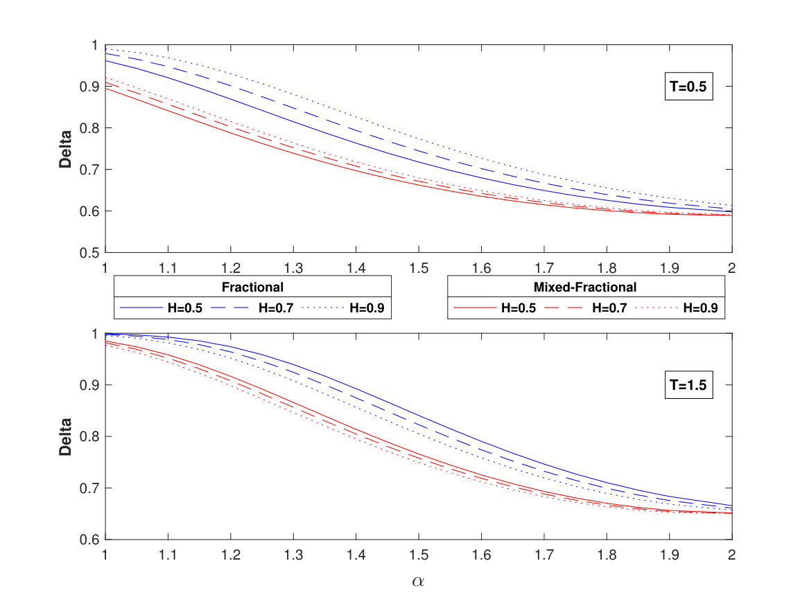 Figure 1
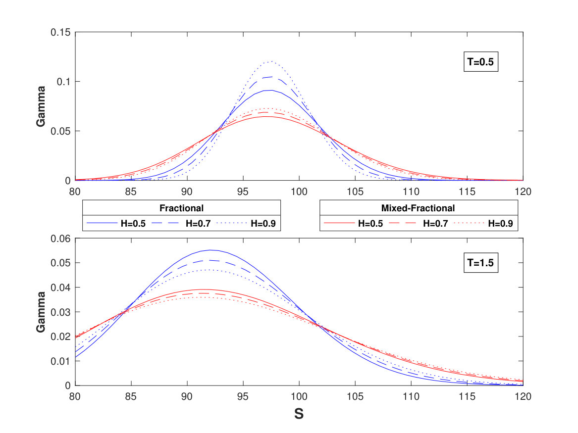 Figure 2
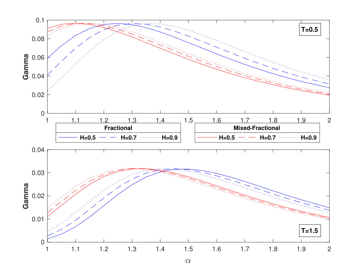 Figure 3
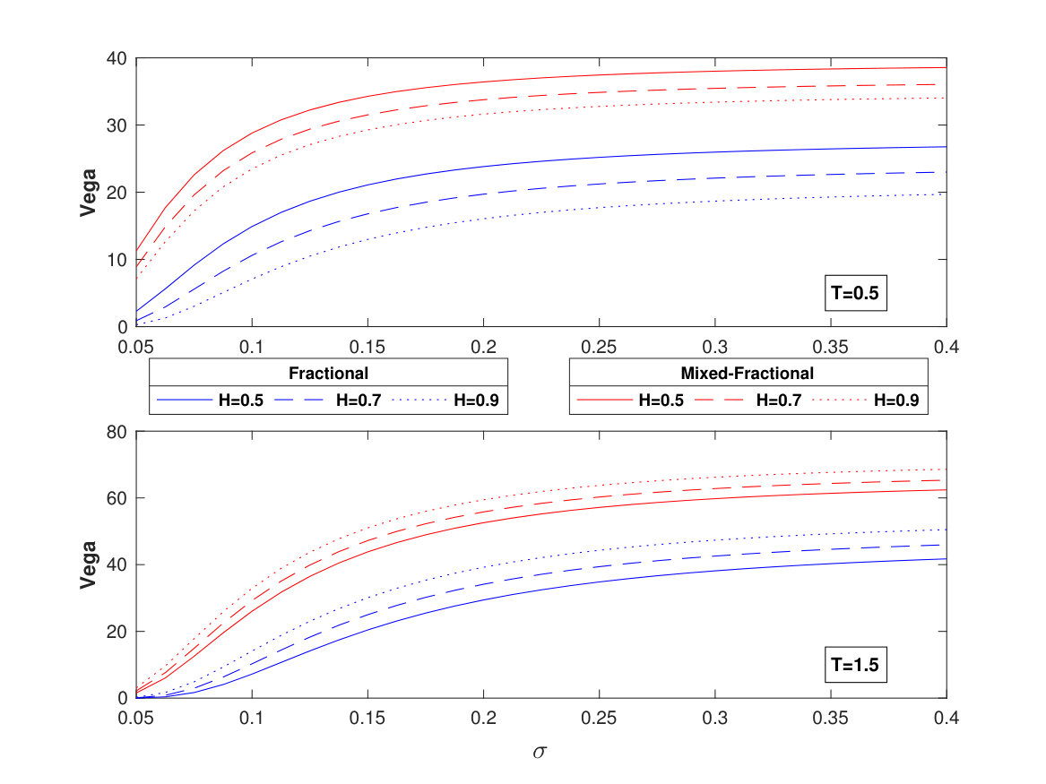 Figure 4
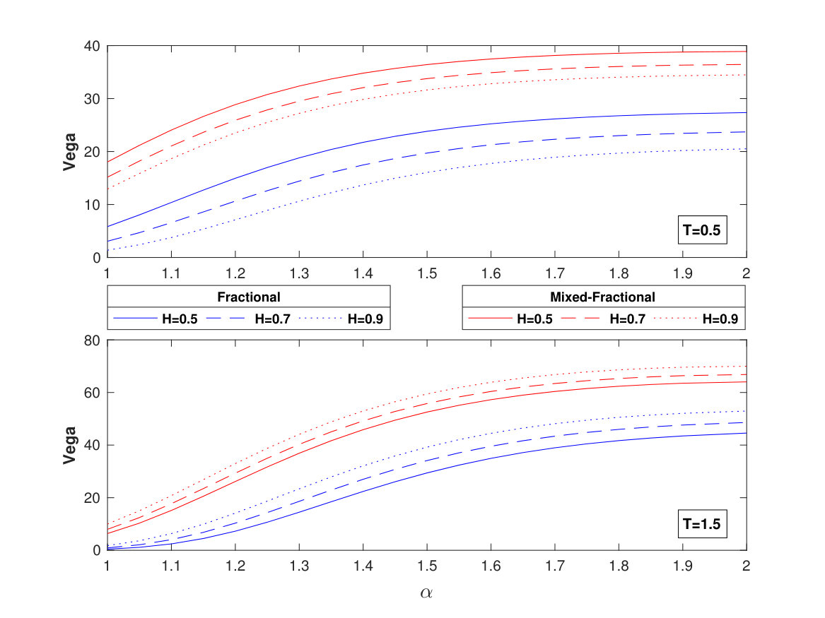 Figure 5
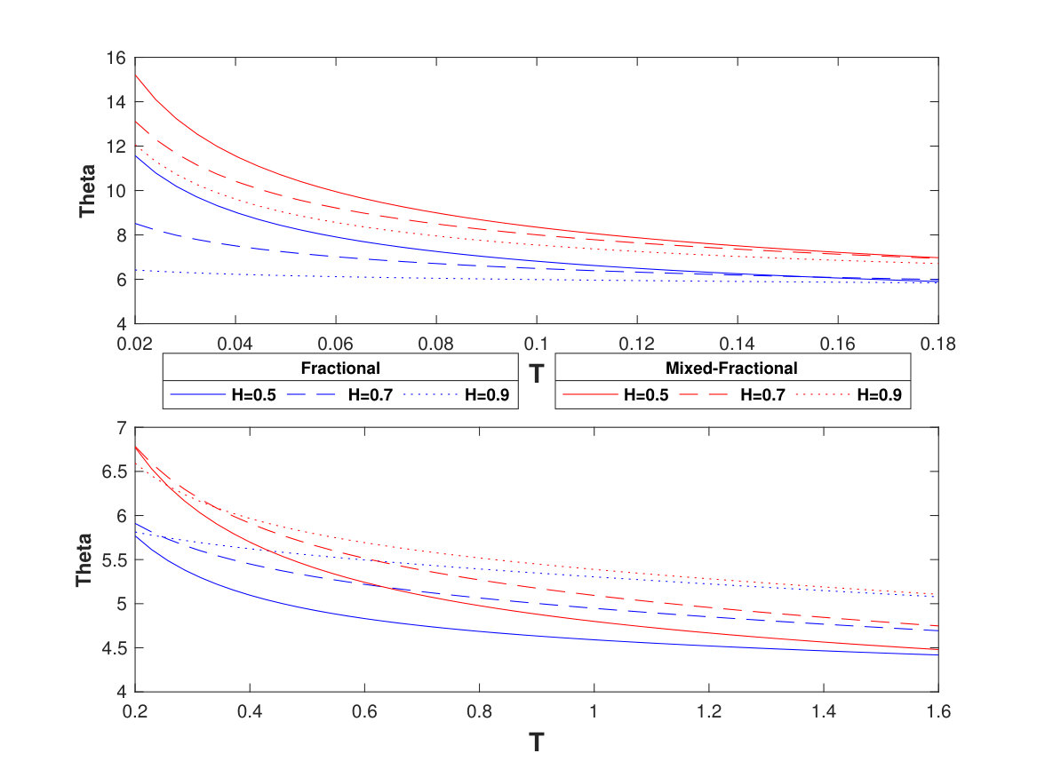 Figure 6
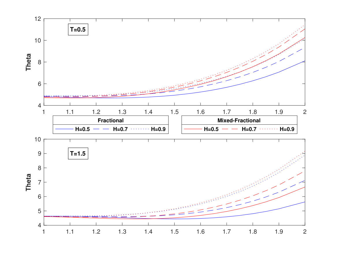 Figure 7
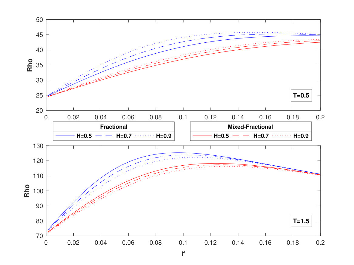 Figure 8
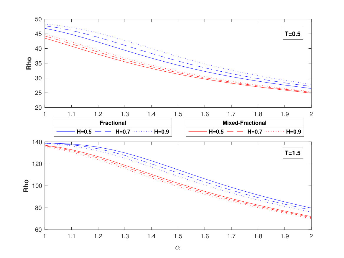 Figure 9
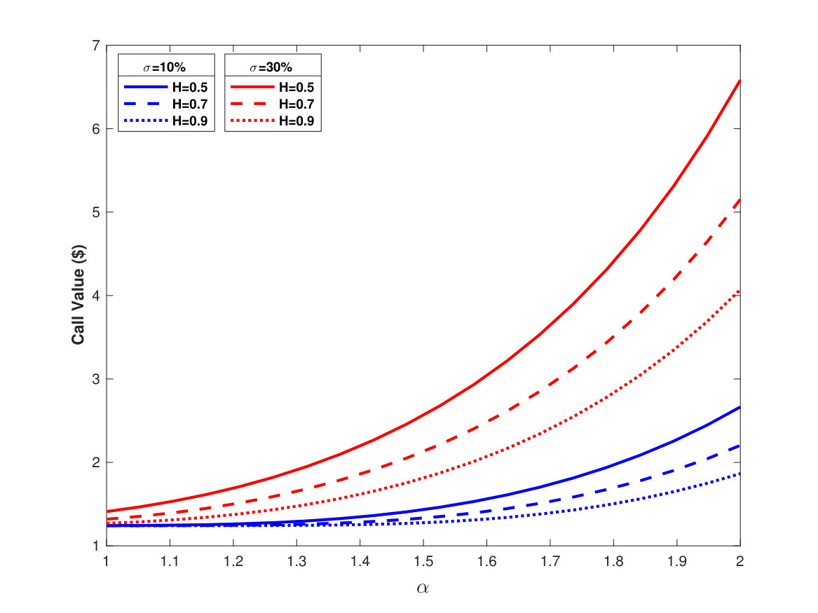 Figure 10
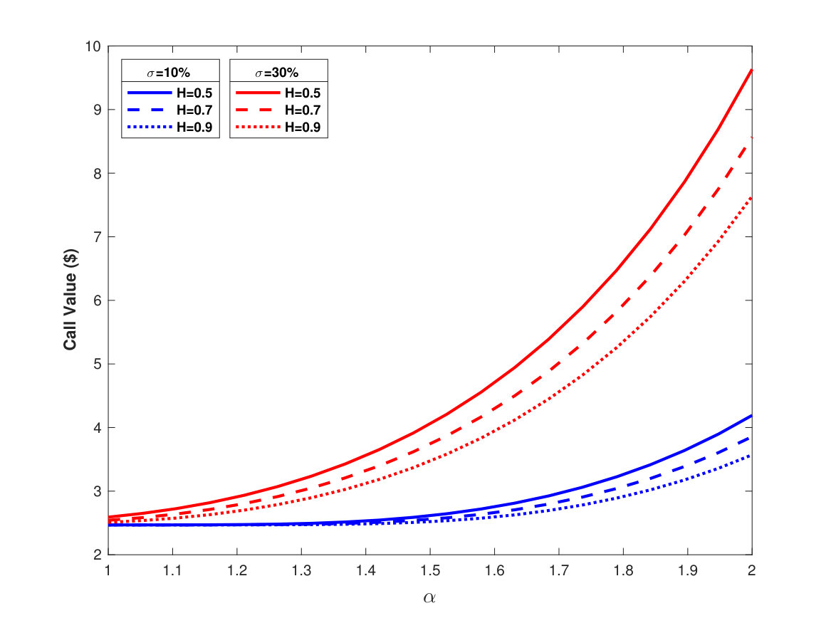 Figure 11
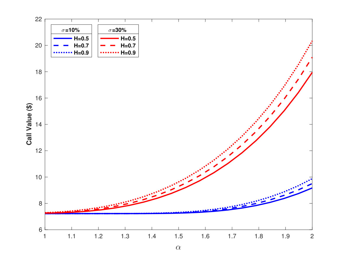 Figure 12
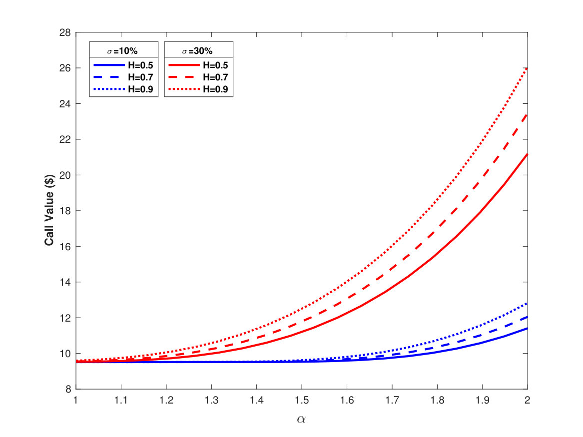 Figure 13
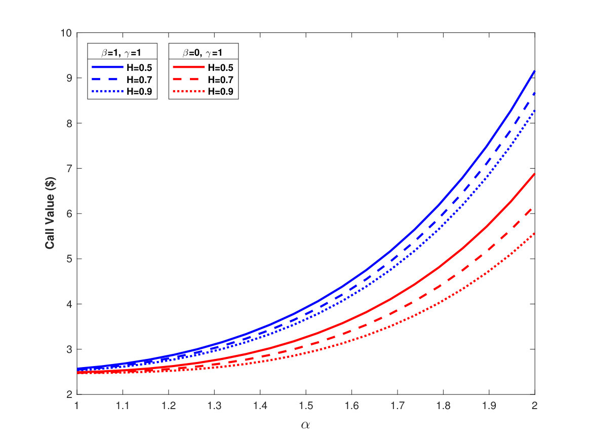 Figure 14
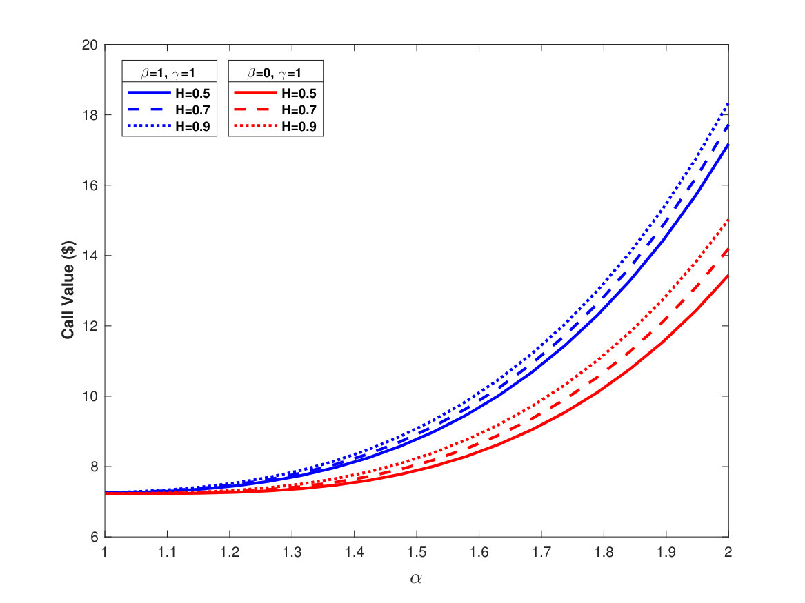 Figure 15
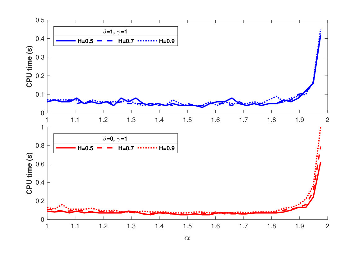 Figure 16
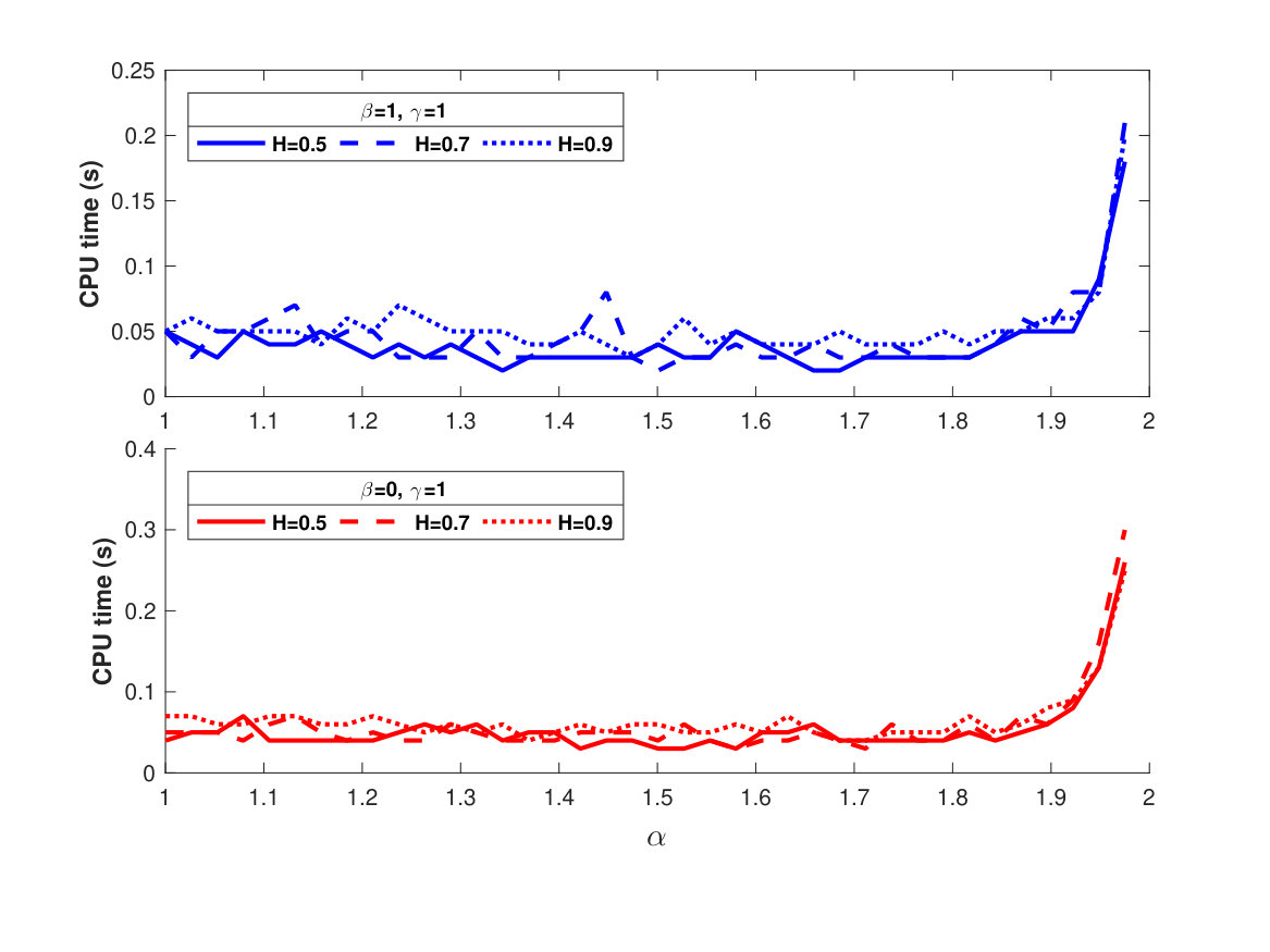 Figure 17
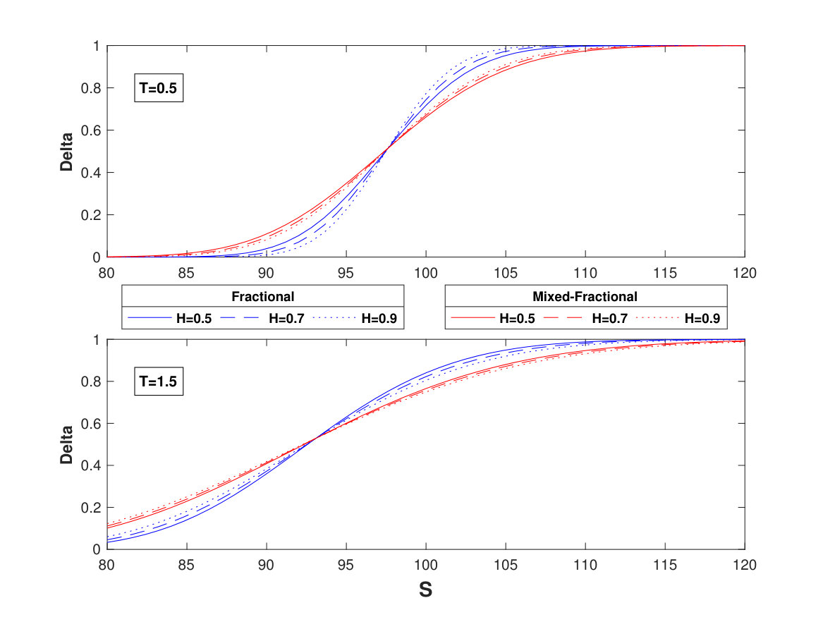 Figure 18
Peer Reviews
No public reviews on file for this paper yet. If you reviewed it on a platform where reviews are public (OpenReview, ICLR, NeurIPS, ICML), you can paste yours below so the community can read it here.
Videos
No videos yet. Explain this paper in a talk, walkthrough, or lecture? Add one.
Taxonomy
TopicsStochastic processes and financial applications · Financial Risk and Volatility Modeling · Complex Systems and Time Series Analysis
The fractional and mixed-fractional CEV model
Axel A. Araneda Email: [email protected], Tel.:+49 69 798 47501
Abstract
The continuous observation of the financial markets has identified some ‘stylized facts’ which challenge the conventional assumptions, promoting the born of new approaches. On the one hand, the long-range dependence has been faced replacing the traditional Gauss-Wiener process (Brownian motion), characterized by stationary independent increments, by a fractional version. On the other hand, the CEV model addresses the Leverage effect and smile-skew phenomena, efficiently. In this paper, these two insights are merging and both the fractional and mixed-fractional extensions for the CEV model, are developed. Using the fractional versions of both the Itô’s calculus and the Fokker-Planck equation, the transition probability density function of the asset price is obtained as the solution of a non-stationary Feller process with time-varying coefficients, getting an analytical valuation formula for a European Call option. Besides, the Greeks are computed and compared with the standard case.
Keywords: fBM, mfBm, CEV, fractional Fokker-Planck, fractional Itô’s calculus, Feller’s process
Frankfurt Institute for Advanced Studies
60438 Frankfurt am Main, Germany.
This version: June 1, 2019
1 Introduction
One of the most important insights in financial mathematics has been the Black-Scholes model [1], which uses a Geometric Brownian motion (GBM) for describes the returns of the asset prices as a regular diffusion process and arriving at an analytical formula for a Vanilla European option.
However, some “Stylized facts” in the financial markets don’t agree with the assumptions using in the Black-Scholes model. One of these findings is the long-range dependence111a.k.a persistence, ‘Memory effect’ or ‘Joseph effect’ [2, 3, 4, 5], motivating the creation of a fractal version of the Black-Scholes model [6, 7], based on fractional Brownian motion [8, 9, 10]. Hu & Øskendal [11] and Necula [12] arrive at an analytical formula for the European Call option for the fractional Black-Scholes case, using Wick-Itô calculus [13, 14]. Nonetheless, in the fractional framework, the arbitrage possibilities aren’t enterely omitted [15, 16, 17]. Addressing it fact, Cheridito [18] introduces the mixed-fractional Brownian motion (see further mathematical details at refs. [19, 20]). This kind of model ensures the absence of arbitrage opportunities [21, 22] and also a pricing formula for European type contracts could be obtained [23, 24].
On the other hand, and come back to shortcomings of the original Black-Scholes model, the homoscedasticity assumption is not consistent with other empirical facts as the volatility smile-skew [25, 26, 27, 28] and leverage effect [29, 30, 31, 32]. The former is the change in the implied volatility pattern as a function of the strike price of an option. The latter is understood as the inverse relationship between the volatility and the price. In this context, a very popular formulation is the Constant Elasticity of Variance (CEV) model developed by Cox [33, 34], which faces the heteroscedasticity and the leverage effect modeling the volatility as a function of the asset price level. The model also deals with the skew-smile phenomena [35, 36]. Despite that the CEV model considers only one more parameter (elasticity) than the Black-Scholes model222See [37] to details on the parameter estimation issue under CEV., the latter is outperformed by the CEV in both prices and option pricing performance [38, 39, 40, 41]. Another plus point to the use of the CEV model is existence of a closed form formula for a European vanilla option. The original Cox’s work derives the Call price in terms of summations of the incomplete gamma function, but later Schroder [42] developed a closed-form solution depending on the non-central distribution333The computation of the non-central chi-squared distribution in Schroeder’s formula is quite unstable and becomes expensive for elasticities near to zero. In order to reduce the computational times and also to address American-type options, several analytical approximations and numerical methods have been developed for the CEV model, see [43, 44] for a survey.. See Refs. [45, 46, 47] for recent and successfully applications of the CEV model in different contexts.
Given the previous statement, the aim of this paper is to merge the local volatility approach and the fractional calculus, extending the CEV model under classical Brownian motion to the fractional and mixed-fractional cases. The fractional CEV case has been addressed previously in the literature [48], proposing a European Call formula in terms of the standard complementary gamma distribution function, similar to the Cox’s result, but without explicit evaluation of the added terms. This time, for the fractional CEV, the European Call price is derived by a compact and explicit way, in terms of the non-central-chi-squared distribution and the M-Whittaker function, following the Schroder scheme and using a time-varying coefficients’ version of the Feller’s diffusion problem. Besides, similarly, a pricing formula for the mixed-fractional CEV model is studied. Also, the convergence of the fractional CEV pricing to the fractional Black-Scholes case is shown. Moreover, the Greeks of the models are computed and compared with the standard CEV case.
The paper outline is the following. First, the CEV model is revisited. Later, the fractional extension is analyzed, deriving the pricing formula for a European Call option. After that, a mixed fractional structure is proposed, arriving at the related European Call pricing formula. At next, the computation and analysis of the Greeks, are performed. Finally, the main conclusions are displayed.
2 The CEV model
Under the risk-neutral measure, at the constant elasticity of variance model, the asset price follows the next stochastic differential equation:
[TABLE]
where and are the constant parameters of the model, with and . is a standard Brownian motion, such that d. In the limit case, when , the CEV turns into the Black-Scholes model.
Aplying the following change of variable:
[TABLE]
and by the Itô’s Lemma, Eq. (1) becomes:
[TABLE]
Let , the transition probability function which rules the evolution of from to , and . Then, evolves according to the Fokker-Planck equation:
[TABLE]
Eq. (3) can be solved by the famous Feller’s lemma [49], summarized at next:
Feller’s lemma**.**
Let u=u(x,t), and a,b,c constants, with a>0 and t>0. The solution of the parabolic equation
[TABLE]
conditional to
[TABLE]
is given by
[TABLE]
where is the modified Bessel function of the first kind of order k.
Proof.
If we set , and ; by the Feller’s Lemma, the transition probability distribution from to , is given by:
[TABLE]
Coming back to the original variables and reordering terms, the density for given is equal to [42]:
[TABLE]
where:
[TABLE]
Later, the value of a Call option at time , with maturity and exercise price , is computed by the Feynman-Kac formula:
[TABLE]
where . As pointed by Schroder [42], the arguments of both integrals are the pdfs of the non-central chi-squared distributions with degrees of freedom and non-centrality parameter , noted by and defined as:
[TABLE]
Back to the pricing equation, the first integral is developed as:
[TABLE]
While the second one:
[TABLE]
Called to the complementary distribution function of :
[TABLE]
and using the following identity[42]:
[TABLE]
the call formula can be wrote as:
[TABLE]
As we remarked previously, the Black-Scholes model can be treated as a limit case of the CEV model, when . For observe the convergence of the solution given in (11) to the Black-Scholes case, we will use the following result for the complementary distribution function , based on the central limit theorem [51]:
[TABLE]
where is the standard normal complementary density function.
Thus, the first complementary function of the Eq. (11), when , is computed as:
[TABLE]
and for the symmetry of the normal function, we have that:
[TABLE]
being the standard normal cumulative density.
The calculus of second function of the Eq. (11), when the degrees of freedom tends to infinity, is:
[TABLE]
and for the identity between de cumulative and complementary function:
[TABLE]
Later, at the limit , the European Call pricing of the CEV model converges to:
[TABLE]
which is the classical Black-Scholes formula provided in [1].
3 A fractional CEV model
Now, to address the ‘Joseph effect’ at the CEV environment, the standard Brownian motion of the Eq. (1) is switched by a fractional one444Following [13], a fBM is a Gaussian process which fulfills (for ; ): i) ii) Then, for , the autocorrelation function of is positive and decays hyperbolically in function of the lags, i.e., long range dependency: .,555Analogously to their classical counterpart, by the fractional Girsanov theorem (see [11, 12, 52]), Eq. (15) is wrote under the risk-neutral measure with drift , where is a fractional Brownian motion. ,666The fractional Brownian motion is not a semi-martingale for ; i.e., there is not an equivalent martingale measure. As pointed in [53], and despite the non-martingale condition, the expected discounted value is equal to the current value.:
[TABLE]
where is a fractional Brownian motion with Hurst exponent .
Considering the shift of coordinates defined in Eq. (2) and the fractional Itô’s formula [54, 55], the Eq. 15 changes to:
[TABLE]
Then, the fractional Fokker-Planck equation [56, 57, 58] related to the stochastic process defined in Eq. (16), is given by:
[TABLE]
Unfortunately, the relation (17) can’t be solved using the Feller’s lemma because the coefficient are time-dependent (i.e, non-constant). However, Masoliver [59] provides an interesting approach for the non-stationary Feller process when the coefficients are time-dependent, and the main useful result for us is provided in the following statement:
Feller’s lemma with time-varying coefficients**.**
Let u=u(x,), A=A(), C=C() and constant defined by
[TABLE]
The solution of the parabolic equation
[TABLE]
conditional to
[TABLE]
is given by
[TABLE]
where is the modified Bessel function of the first kind of order k and
[TABLE]
Proof.
See Ref. [59].
∎
So, if we use the previous definitions of (cf. page Feller’s lemma), and set:
[TABLE]
Eq. (17) transforms into:
[TABLE]
and , a constant.
Then, Eq. (21), can be solved by the Feller’s lemma with time-varying coefficients. Indeed:
[TABLE]
where:
[TABLE]
and is the M-Whittaker function777The Whittaker (or confluent hypergeometric) function appears in the solution of other related problems that involve the CEV process, see for example [60, 61, 62], among others. [63, 64, 65] and can be expressed in terms of the confluent hypergeometric Kummer’s function:
[TABLE]
Now, solving for the original time-coordinate, at time , we have:
[TABLE]
with
[TABLE]
Later, moving to the original frame of reference , and replacing the values for a,$$b and , the probability density function of , given is:
[TABLE]
being:
[TABLE]
The transition probabilities (Eq. (5)) and (Eq. (22)) differ only by the terms and . For the particular case , these terms are equal888
\displaystyle\phi(t)\biggr{|}_{H=1/2}=\frac{a}{b}\left(\text{e}^{bt}-1\right)
\displaystyle k_{H}\biggr{|}_{H=1/2}=\frac{b}{a\left(\text{e}^{bT}-1\right)}=k
, yield to P=P_{H}\Bigr{|}_{H=1/2} .
After that, a European option price may be computed taking expectations of the discounted payoff (see appendix A). Fixing , and following the development given from the Eq.(9) to the Eq. (11), the pricing for a European call , in the fractal CEV, becomes:
[TABLE]
Using the derivatives, asymptotics and recurrence properties999Mainly, we use:
•
•
{\displaystyle\frac{\text{\partial}}{\partial l}}M_{\kappa,\upsilon}\left(l\right)=\left(\frac{1}{2}-\frac{\kappa}{l}\right)M_{\kappa,\upsilon}\left(l\right)+l^{-1}\left(\frac{1}{2}+\kappa+\upsilon\right)M_{\kappa+1,\upsilon}\left(l\right)
•
of both and [65], from (26) an interesting result is obtained computing the limit case . By Eq. 12, we get:
[TABLE]
[TABLE]
and replacing in (26), we arrive at the fractional Black-Scholes formula [11, 12]:
[TABLE]
Then, the convergence of the CEV to the Black-Scholes model, in the limit case remains in the fractional scheme.
Fig. 1 plots the values of the fractional CEV formula for equal to 15% (blue) and 30% (red), and three values of ={0.5, 0.7, 0.9} considering different maturities. The solid lines draw the case , which corresponds to the classical CEV pricing. The semi-solid and dotted lines show the pricing using and , respectively. The fractional CEV retains the property of being a monotonically increasing function of the elasticity parameter. Also, is a rising function of and . For expiration times below the year (Figs. 1a-1b), the option price falls if moves to 1. In the opposite way, for (Figs. 1c-1d), the prices grow if rise in the interval [1/2,1[. When , the fractional CEV pricing transforms into the fractional Black-Scholes price.
4 A mixed-fractional CEV model
A mixed-fractional Brownian motion, is defined as a linear combination between an standard Brownian motion and other independent and fractional Brownian motion101010Cheridito [18] proves that for the filtration generated by is equivalent to a classical Brownian motion; i.e, a semi-martingale.:
[TABLE]
Then, for to extent the CEV model to the mixed-fractional case, the Brownian motion which drives the CEV model is replaced by :
[TABLE]
Is clear that if we recover the fractional case studied in the previous section. Also, if and , Eq. (29) describes the classical CEV model (Sec. 2).
Analogous to the previous cases, the transformation (2) and the fractional Itô’s lemma goes Eq. (29) to:
[TABLE]
Since that , the fractional Fokker-Planck equation for the above process is:
[TABLE]
Setting:
[TABLE]
the relation (30) becomes:
[TABLE]
where , are given by Eqs. (18)-(20).
Given that (constant), a solution for (31) is obtained through the Feller’s lemma with time-varying coefficients:
[TABLE]
and
[TABLE]
Later, the transition probability density function for conditional to , under a mixed-fractional regime is given by:
[TABLE]
being :
[TABLE]
with,
[TABLE]
Using the argument provided in the previous sections, the European Call price, at time under the mixed-fractional CEV framework is computed by:
[TABLE]
where .
Eq. (35) turns into the pure fractional CEV case (Eq. (26)) if , and becomes the classical CEV model if or .
Using the results computed in the Eqs. (13), (14), (27) and (28); at the limit case Eq.(35) tends to:
[TABLE]
with
[TABLE]
[TABLE]
which is the mixed-fractional Black-Scholes pricing formula (for instance, see [24] with and ); keeping the convergence between the CEV and Black-Scholes.
Fig. 2 display the value for a European Call under the mixed-fractional CEV model, setting the pair of coefficients and as and (blue and red respectively), with the aim of to compare the mixed fractional and pure fractional cases. We consider two maturities T=0.5 (2a) and T=1.5 (2b) and . In both subplots the classical CEV pricing is represented by the red-solid-line. We can observe that the mixed-fractional price is higher than the both classical and fractional price. As in the pure fractional case, for T<1 the price decreases if H tends to one, and increases for T>1 and H moves to one.
Fig. (3) addresses the computational cost, measured as CPU time, of the mixed and pure fractional models. For , the formula becomes extremely expensive. Nevertheless, there are no significative differences in terms of cost between the classical and fractional approaches.
5 Greeks
For to analyze the sensitivities of the pricing formula as function of the parameters of the model, we compare the Greeks of both classical, fractional and mixed-fractional CEV models.
The most common sensitivities are related to the price, maturity, volatility and interest rate. We use the results given in Ref. [44] for , , and Greeks under the classical CEV model and here we carefully extent it to the fractional cases.
5.1 Delta
[TABLE]
where is the non-central- PDF defined in 10.
For the fractional case, we have:
[TABLE]
and in the mixed-fractional:
[TABLE]
The charts at the Figure 4 show the behavior of the \text{\Delta,}\,\Delta_{H} and varying the spot price (4a) and elasticity (4b) for maturities below and above the unity. The solid blue line corresponds to the classical CEV model.
5.2 Gamma
The eqs. 39, 40 and 41 provide the Gamma sensitivity for standard, fractional and mixed-fractional CEV, respectively, plotting it at Fig. 5
[TABLE]
[TABLE]
[TABLE]
5.3 Vega
The partial derivative with respect to the volatility is called Vega (commonly represented by the greek letter ). In the CEV model, the volatility is a function of both and the parameter , defined by . Then the Vega for the CEV model is:
[TABLE]
For the fractional and mixed-fractional models, we have:
[TABLE]
[TABLE]
The graphics in Fig. 6 display the Vega for the fractional and mixed-fractional models. The standard CEV Vega is plotted by the solid-blue line.
5.4 Theta
The change rate of the option price with respect to the maturity is noted by the greek , and is computed for the CEV model at the Eq. 45, for the fractional CEV at Eq. 46 and for the mixed-fractional CEV at Eq. 47. Fig. 7 draw the shape of and under different values of T (7a) and alpha (7b).
[TABLE]
[TABLE]
[TABLE]
5.5 Rho
Finally, the sensitivity respect to the risk-free-interest rate, for the CEV model and its extensions (fractional and mixed-fractional), are shown at Fig. 8 and explicitly computed at the eqs. 48-49-50.
[TABLE]
[TABLE]
[TABLE]
6 Summary
In this paper, the constant elasticity of variance model is studied, adding a fractal feature to the Brownian motion to address the long-memory in financial markets. Besides, to deal with the non-arbitrage issue under pure fractional regimes, a mixed fractional CEV model is developed.
Then, using the fractional Itô calculus and the fractional generalization of the Fokker-Planck equations, an analytical and compact option pricing scheme for a European Call, based on the complementary non-central-chi-squared density function and the M-Whittaker function, is provided for both approaches. The convergence to both the classical CEV model and the fractional & mixed-fractional Black Scholes formula are shown for the limit cases and , respectively, and then the proposed fractional extensions could be interpreted as a generalization of the classical CEV and Black-Scholes model. Besides, the Greeks are computed showing their behavior under different values of the Hurst exponent, considering maturities lower and greater than one.
Since the added terms on the call formula in both fractional models, in relation to the classical CEV, doesn’t have a dependency on the strike price, the fractional and mixed-fractional CEV keep the capability to address the smile-skew issue.
7 Acknowledgements
I thank FIAS for financial support and both Dr. Nils Bertschinger and Dr. Marcelo Villena for helpful discussions.
Appendix A Risk-neutral pricing in the fractional
CEV model
As pointed in [11, 12], the fractional Clark-Ocone theorem and quasi-expectations are used for to price a derivative under fractional Brownian motion. Here, we use the derivation of Hu and Øskendal [11] for to obtain a risk-neutral pricing at time , but using a fractional CEV approach instead a fractional GBM.
Since the market is complete, at time , a derivative is replicated by:
[TABLE]
where and are weights, is a money bank account (bond) which pays a continuously composed interest rate (risk-less interest rate; i.e, ) and is ruled by the Eq. 15.
Later:
[TABLE]
Multiplying 52 by and integrating it from zero to , we get:
[TABLE]
On the other hand, the Clark-Ocone theorem for standard Brownian motions is given by [66]:
[TABLE]
where is the Malliavin derivative and is the natural filtration of Brownian motion. The fractional extension of the Eq. is provided by Refs. [11, 67]:
[TABLE]
being the -algebra generated by , . Put in 54:
[TABLE]
Comparing the expressions 53-55 we arrive to the completeness of the market by:
[TABLE]
and
[TABLE]
Then, at the initial time, the price of a derivative is computed discounted the expected value, as in the classical model driven by a Brownian motion.
For the mixed-fractional case, the extension is straightforward and is shown in [23, 68] for the mixed GBM.
The reference list from the paper itself. Each links out to its DOI / PubMed record.
- 1[1] Fischer Black and Myron Scholes. The pricing of options and corporate liabilities. Journal of Political Economy , 81(3):637–654, 1973.
- 2[2] Andrew W. Lo. Long-term memory in stock market prices. Econometrica , 59(5):1279–1313, 1991.
- 3[3] Walter Willinger, Murad Taqqu, and Vadim Teverovsky. Stock market prices and long-range dependence. Finance and stochastics , 3(1):1–13, 1999.
- 4[4] Shibley Sadique and Param Silvapulle. Long-term memory in stock market returns: international evidence. International Journal of Finance & Economics , 6(1):59–67, 2001.
- 5[5] Daniel O Cajueiro and Benjamin M Tabak. The hurst exponent over time: testing the assertion that emerging markets are becoming more efficient. Physica A: Statistical Mechanics and its Applications , 336(3-4):521–537, 2004.
- 6[6] Nigel Cutland, P. Ekkehard Kopp, and Walter Willinger. Stock price returns and the Joseph effect: a fractional version of the Black-Scholes model. In Seminar on stochastic analysis, random fields and applications , pages 327–351. Springer, 1995.
- 7[7] W Dai and CC Heyde. Itô’s formula with respect to fractional brownian motion and its application. International Journal of Stochastic Analysis , 9(4):439–448, 1996.
- 8[8] Benoit B. Mandelbrot and John W. Van Ness. Fractional Brownian motions, fractional noises and applications. SIAM review , 10(4):422–437, 1968.