H-, He-like recombination spectra III: $n$-changing collisions in highly-excited Rydberg states and their impact on the radio, IR and optical recombination lines
F. Guzm\'an, M. Chatzikos, P. A. M. van Hoof, Dana S. Balser, M., Dehghanian, N. R. Badnell, G.J. Ferland

TL;DR
This paper investigates the impact of uncertainties in $n$-changing collisional rates on the prediction of radio, IR, and optical recombination lines in gaseous nebulae, showing errors are generally below 5% but can reach 20% in maser-affected cases.
Contribution
It provides a detailed analysis of how different datasets of collisional rates affect the modeling of recombination spectra and quantifies the resulting errors in various astrophysical environments.
Findings
Uncertainties in collisional rates cause less than 5% error in most cases.
Errors can reach up to 20% in maser amplification scenarios.
Simulations of AGN BLRs and Orion Nebula support these conclusions.
Abstract
At intermediate to high densities, electron (de-)excitation collisions are the dominant process for populating or depopulating high Rydberg states. In particular, the accurate knowledge of the energy changing (-changing) collisional rates is determinant for predicting the radio recombination spectra of gaseous nebula. The different datasets present in the literature come either from impact parameter calculations or semi-empirical fits and the rate coefficients agree within a factor of two. We show in this paper that these uncertainties cause errors lower than 5% in the emission of radio recombination lines (RRL) of most ionized plasmas of typical nebulae. However, in special circumstances where the transitions between Rydberg levels are amplified by maser effects, the errors can increase up to 20%. We present simulations of the optical depth and H line emission of Active…
Click any figure to enlarge with its caption.
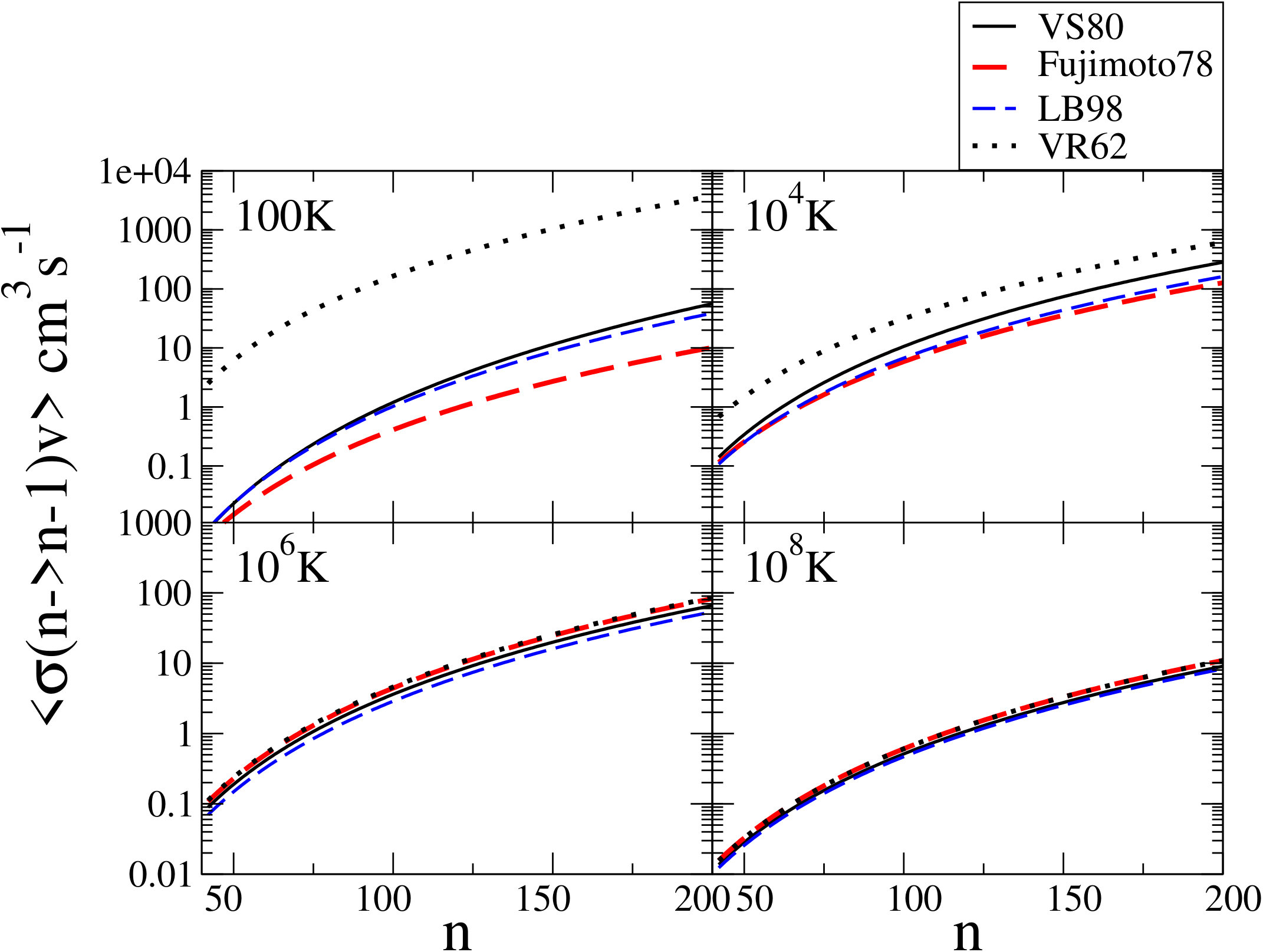 Figure 1
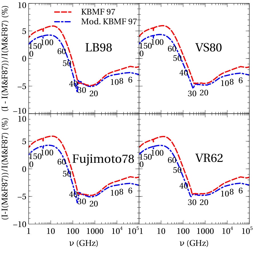 Figure 10
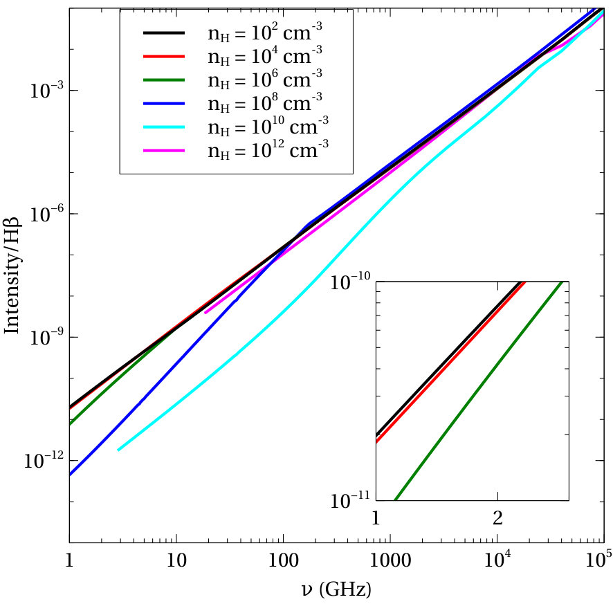 Figure 11
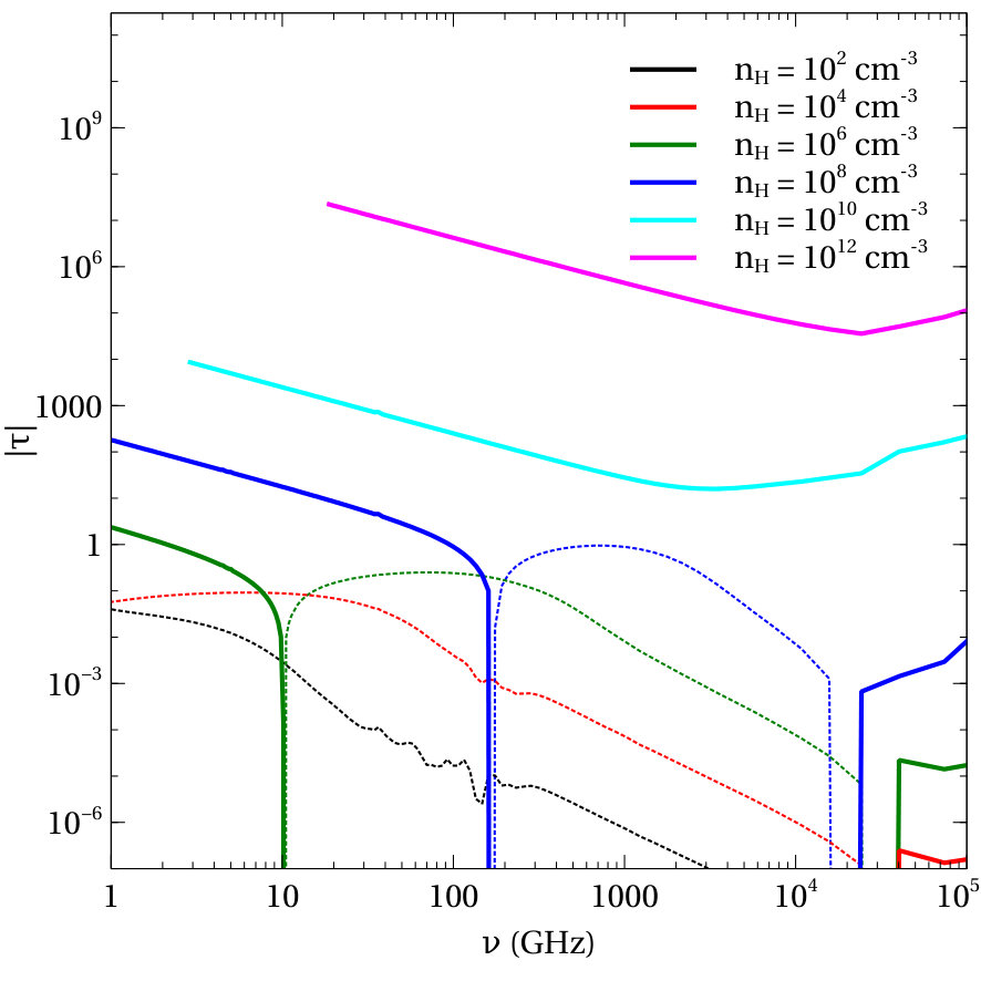 Figure 12
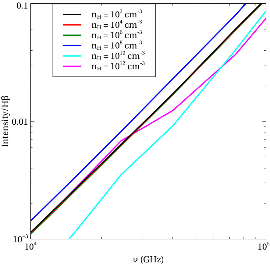 Figure 13
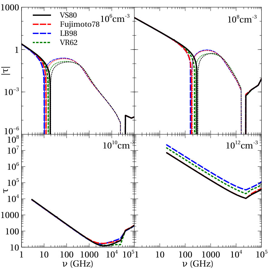 Figure 14
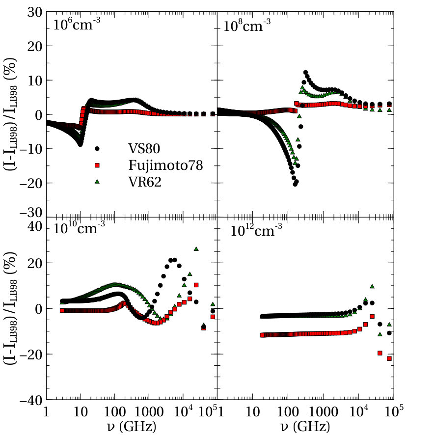 Figure 15
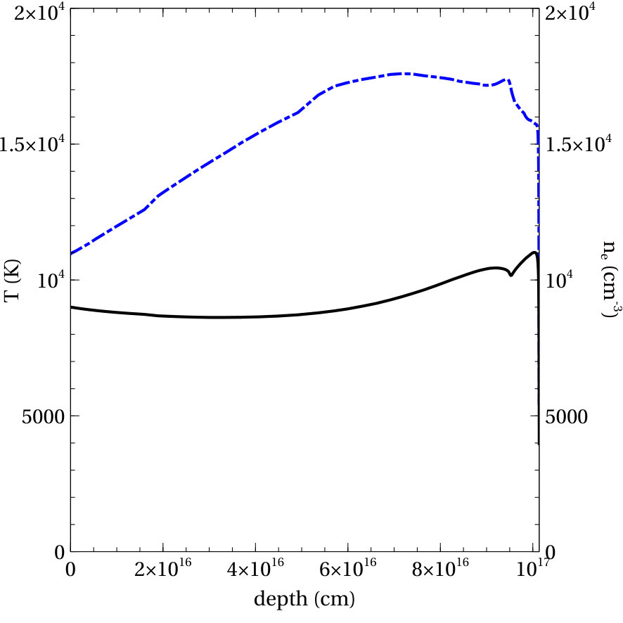 Figure 16
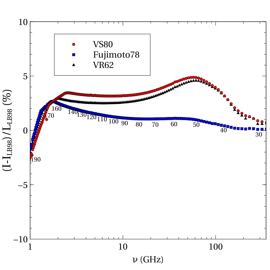 Figure 17
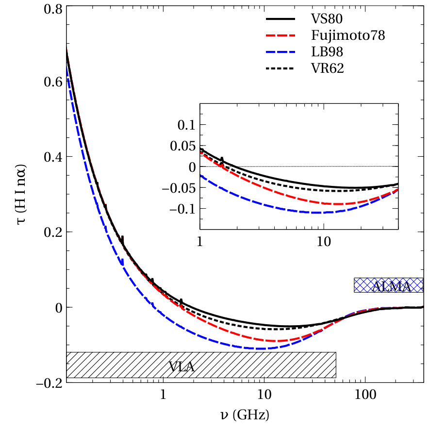 Figure 18
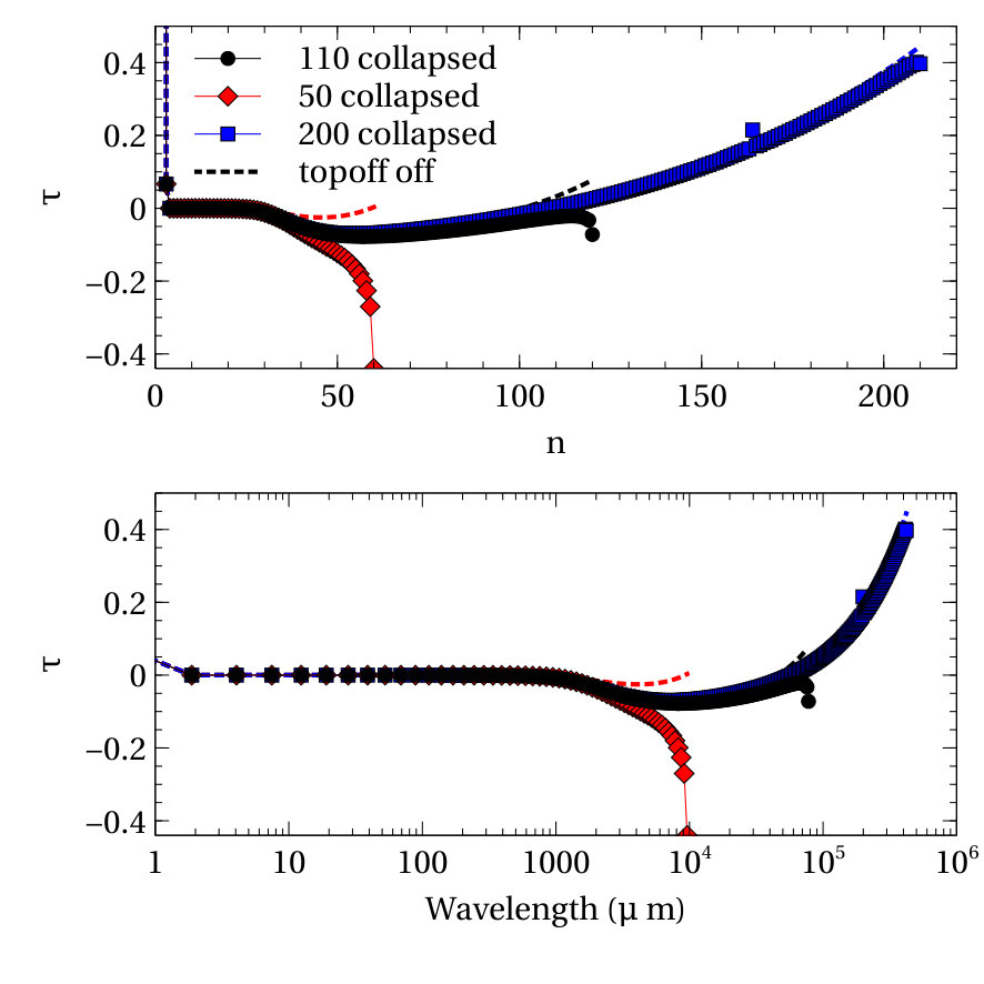 Figure 19
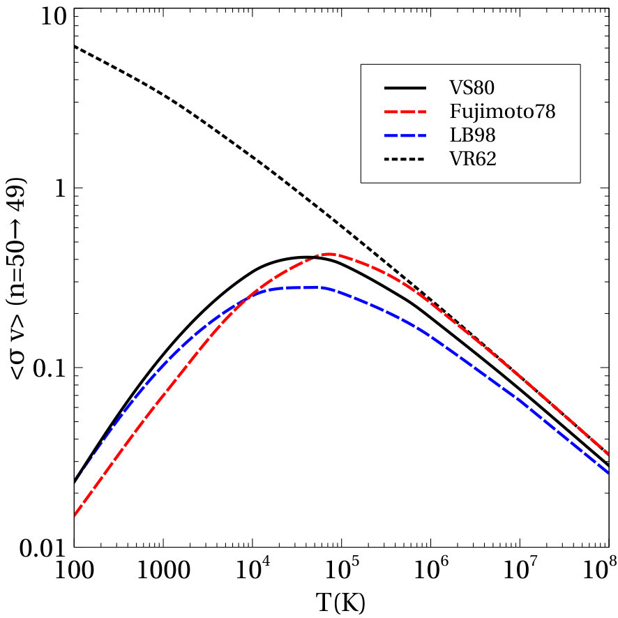 Figure 2
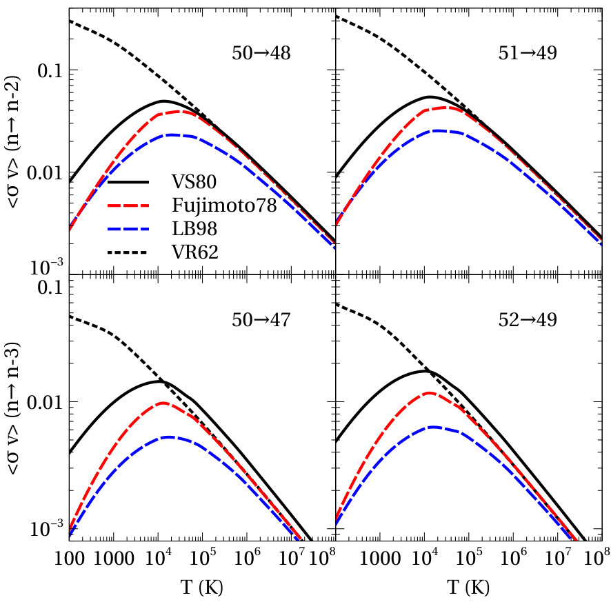 Figure 3
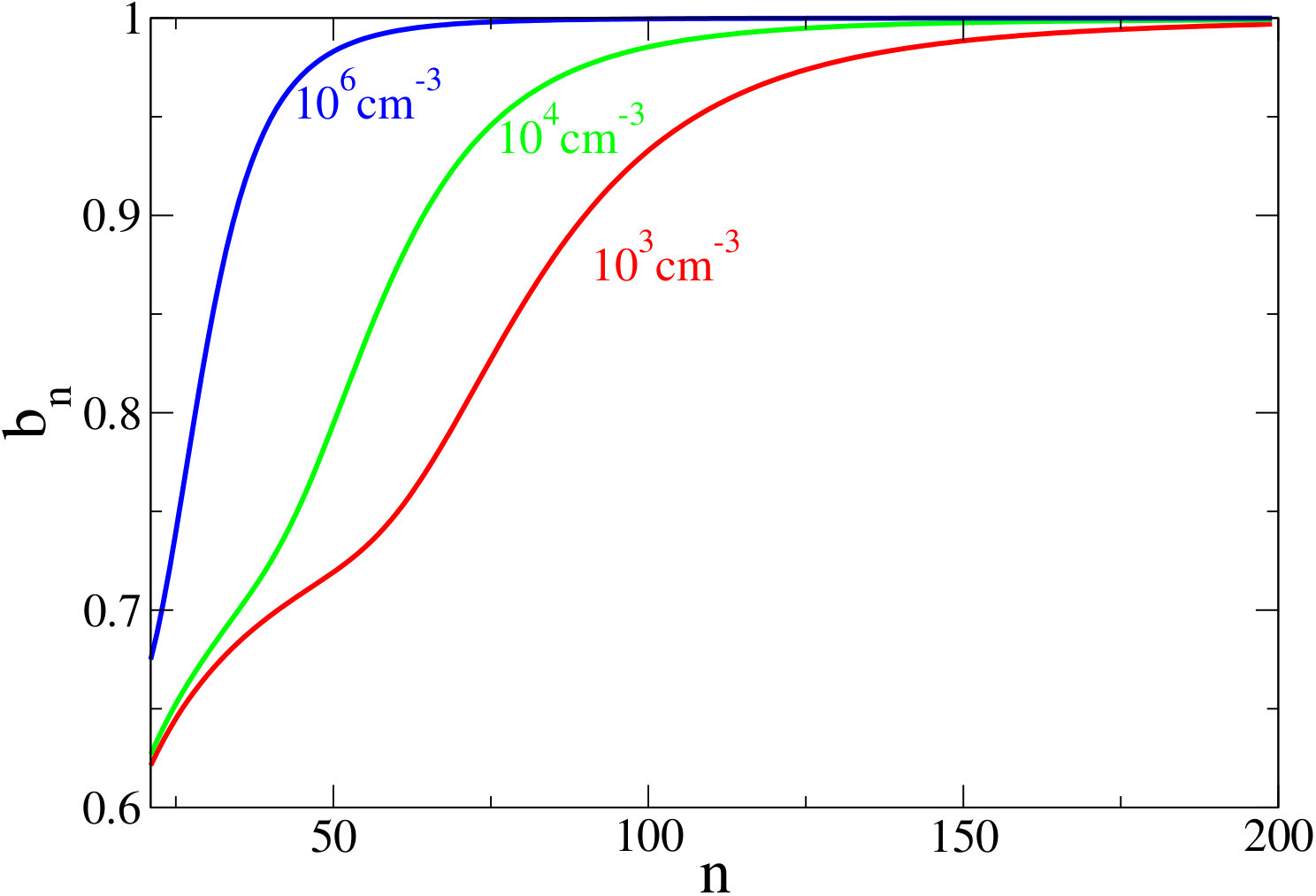 Figure 4
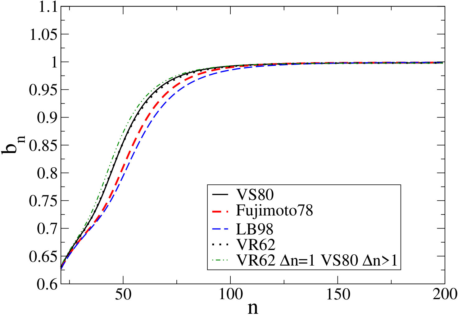 Figure 5
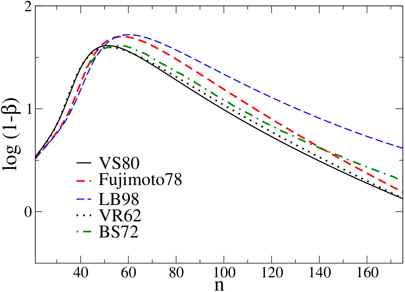 Figure 6
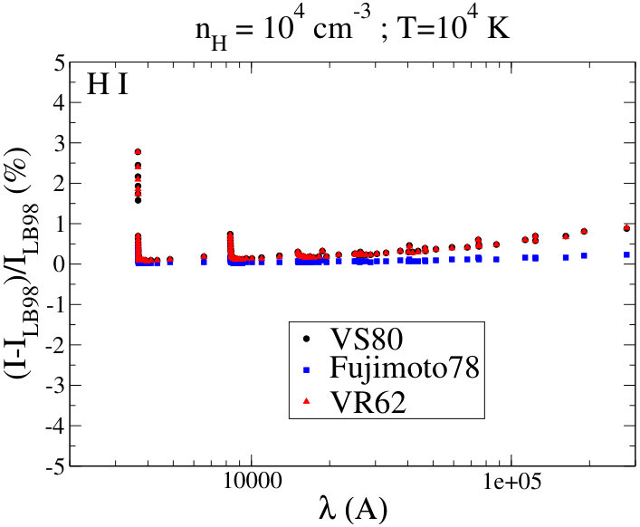 Figure 7
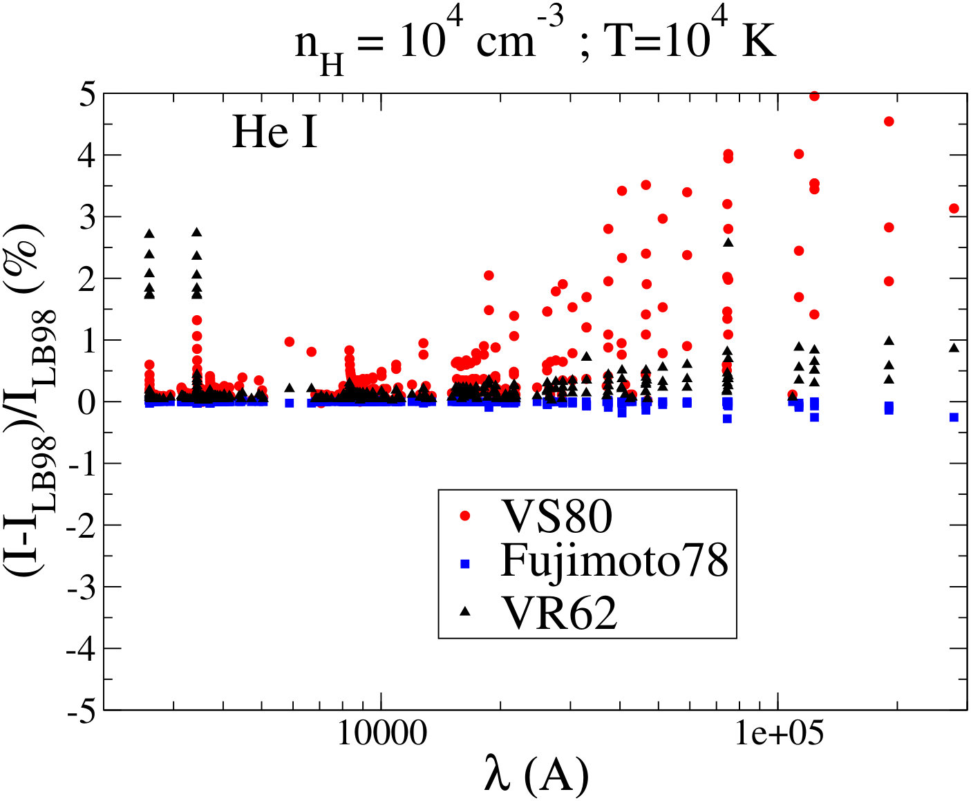 Figure 8
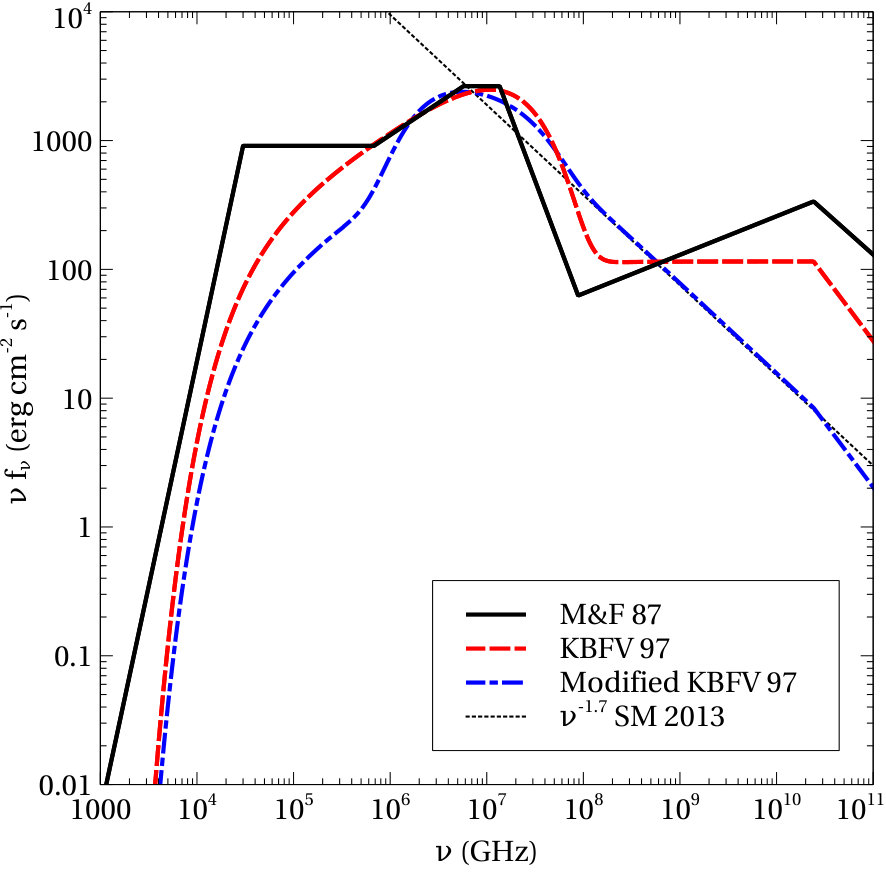 Figure 9
| Ion/Atom | Critical density (cm-3 ) | |
|---|---|---|
| H0 | 383 | 54 |
| He0 | 194 | 23 |
| He+ | 18903 | 2605 |
| C4+ | ||
| C5+ | ||
Peer Reviews
No public reviews on file for this paper yet. If you reviewed it on a platform where reviews are public (OpenReview, ICLR, NeurIPS, ICML), you can paste yours below so the community can read it here.
Videos
No videos yet. Explain this paper in a talk, walkthrough, or lecture? Add one.
H-, He-like recombination
spectra III: -changing collisions in highly-excited Rydberg states and their impact on the radio, IR and optical recombination lines
F. Guzmán1, M. Chatzikos1, P. A. M. van Hoof3, Dana S. Balser2, M. Dehghanian1, N. R. Badnell4 and G.J. Ferland1.
1Department of Physics and Astronomy, University of Kentucky, Lexington, KY 40506, USA.
2NRAO, Charlottesville, VA 22903-2475.
3Royal Observatory of Belgium, Ringlaan 3, 1180 Brussels, Belgium.
4Department of Physics, University of Strathclyde, Glasgow G4 0NG, UK.
(In preparation )
Abstract
At intermediate to high densities, electron (de-)excitation collisions are the dominant process for populating or depopulating high Rydberg states. In particular, the accurate knowledge of the energy changing (-changing) collisional rates is determinant for predicting the radio recombination spectra of gaseous nebula. The different datasets present in the literature come either from impact parameter calculations or semi-empirical fits and the rate coefficients agree within a factor of two. We show in this paper that these uncertainties cause errors lower than 5% in the emission of radio recombination lines (RRL) of most ionized plasmas of typical nebulae. However, in special circumstances where the transitions between Rydberg levels are amplified by maser effects, the errors can increase up to 20%. We present simulations of the optical depth and H line emission of Active Galactic Nuclei (AGN) Broad Line Regions (BLRs) and the Orion Nebula Blister to showcase our findings.
keywords:
(ISM:) H II regions – atomic data – atomic processes – masers – radio lines: general – submillimetre: general
††pagerange: H-, He-like recombination spectra III: -changing collisions in highly-excited Rydberg states and their impact on the radio, IR and optical recombination lines–References
1 Introduction
Radio observations are an important tool in astronomy as the spectrum is not affected by dust extinction. Radio recombination lines (RRL) coming from highly-excited Rydberg levels are used to determine the temperatures and densities of gaseous nebulae (see for example Osterbrock & Ferland, 2006), the metallicity structure of the Galaxy (Balser et al., 2015, 2011), to survey the H II regions of our Galaxy (Anderson et al., 2018) and determine their structure (Anderson et al., 2015; Poppi et al., 2007), to probe extragalactic Active Galactic Nuclei (AGN) and startburst galaxies (Scoville & Murchikova, 2013), to study the Photo-Dissociation Regions (Luisi et al., 2017), and to study the diffuse ionized gas in H II regions and the diffuse clouds of the cold neutral medium (Morabito et al., 2014).
In particular, hydrogen and helium RRL can be used to obtain the electron temperature . If the levels involved in the line transition are close to local thermodynamic equilibrium (LTE), can be obtained directly from the ratio of the line brightness temperature to the continuum brightness temperature (Rohlfs & Wilson, 2000). However, non-LTE effects can be important for RRL (Brown et al., 1978). Likewise, stimulated emission (maser effects) and pressure broadening effects can alter the equilibrium of lines (Shaver, 1980). In these cases, modeling of the level populations using collisional radiative (CR) modeling (Dupree & Goldberg, 1970; Brocklehurst & Seaton, 1972; Burgess & Summers, 1976) is needed to obtain the correct line intensities. CR modeling is subject to the availability and accuracy of the fundamental atomic data describing the processes between the different particles of the emitting gas. The highest uncertainties come from the collisional (de-)excitation, which can be divided into two types of interaction: energy changing and angular momentum changing. In the previous two papers of this series, devoted to investigate and assess these collisional data, which have a high impact on astronomical observations (Guzmán et al., 2016, 2017, hereafter Paper I and Paper II), we showed how the disparities in the theoretical values of -changing collisions cross sections can affect the emissivities of the optical recombination lines. -changing collisions are mainly produced by ion impact and alter the angular momentum of the target electron by Stark mixing without changing its energy (Pengelly & Seaton, 1964). As shown in Paper I and Paper II, at high Rydberg states, -changing collisions are so fast that they populate the subshells statistically, and differences of one order of magnitude between the values of the rate coefficients are not important. However, as noted by Salgado et al. (2017), the low densities of the cold neutral medium make the Stark effect interactions of -changing collisions important at the high levels involved in RRL.
This paper is the third of the series and is focused on electron impact excitations changing the principal quantum number of the target electron. These energy changing electron collisions redistribute the electronic population of the high Rydberg levels of ions and atoms towards LTE. However, many of the Rydberg states will remain in non-LTE. These effects will mainly depend on the accuracy of the electron-impact excitation rate coefficients, which can significantly influence the derived opacities and the temperature diagnostics obtained with RRL. Unfortunately there are no precise quantum calculations for collisional excitation of high Rydberg levels. R-matrix calculations for -changing collisional data for hydrogen- and helium-like (H-like and He-like) iso-sequences reach up to (Anderson et al., 2000; Bray et al., 2000; Ballance et al., 2006; Ralchenko et al., 2008; Griffin & Ballance, 2009). Analytic formulas using the Born approximation (Lebedev & Beigman, 1998) and fitting formulas from theoretical and experimental data (Fujimoto, 1978; Vriens & Smeets, 1980) have been used for transitions with higher .
In this paper, we analyze the impact of the different approaches for -changing electron-impact excitation cross sections on the Rydberg populations of H- and He-like ions and on the RRL. Our main goal is to identify the best data and quantify how the determination of the physical parameters derived from the observed RRL can be compromised by the uncertainty in the -changing collisions. In Section 2, the different approximations are discussed and compared. In Section 3, we discuss how the different values of -changing rate coefficients translate to the populations densities and the predicted RRL intensities and opacities. In that Section, we analyze a simple slab of irradiated gas using the spectral simulation code Cloudy, last described by Ferland et al. (2017). The uncertainties on the excitation rates at high Rydberg levels could affect the lower levels by cascading decay, and thus compete with the errors from the collisional data for low lying levels. We discuss these effects on the uncertainty of the predicted emissivities of optical recombination lines in Section 4. In Section 5.1 and 5.2 we apply our analysis to models of the Broad Line Regions (BLRs) in AGN and the Orion nebula emission, respectively. Finally, we summarize our results in the conclusions.
2 Rydberg collisional excitation theories
Electron-impact excitation between high Rydberg () levels have received considerably less attention than between low-lying -shells due to a number of reasons. First, the low-lying transitions in the optical part of the spectrum are much brighter than the radio lines and less affected by pressure broadening. Line ratios are routinely used in the optical to obtain temperatures and densities. Second, dust absorption and scattering peaks at the mid infrared and is still big at the far infrared (Osterbrock & Ferland, 2006) making intermediate-high Rydberg levels transitions unobservable in dusty environments. Third, the numerical and computational limitations of the theoretical methods prevent accurate quantum calculations for transitions to higher levels. For example, in most R-matrix calculations, including higher levels requires the appropriate inclusion of pseudostates to correctly cover excitation in the close coupling terms. The number of pseudostates needed will grow with the inclusion of more levels. Ballance et al. (2006) show how including the coupling to pseudostates modified their results between 40% – 60%. Finally, in very low density environments, such as in the interstellar medium (ISM), low levels recombine faster and the Rydberg levels eventually decay radiatively to lower levels. At high densities, collisions are so fast that the levels are expected to be in LTE independently of the value of the collisional transition probability, so the actual theory is unimportant. However, there is a wide number of astrophysical circumstances where the Rydberg levels can be in non-LTE and their populations driven by the rates of electron impact collisions (e.g. see Sections 3 and 5).
2.1 Collisional excitation datasets
Maxwell-averaged collisional effective rate coefficients for the dominant de-excitations, where is the principal quantum number of Rydberg states, are plotted in Figures 1 and 2 for neutral atoms and for K as a function of the upper level main quantum number and the electron temperature respectively. While the curves have a similar shape (with the exception of the VR62 set explained later in this section, they differ from 30% at high temperatures to 60% at K. In this paper we investigate whether these uncertainties could impact predictions of astrophysical interest.
2.1.1 VR62
van Regemorter (1962) obtained new values for the experimentally averaged Gaunt factor approximation proposed by Seaton (1959). The effective rates for de-excitation proposed by this model are:
[TABLE]
where is the electron temperature in K, (cm), with the Planck constant and the speed of light, is the transition energy, is the Einstein coefficient, , and
[TABLE]
with , the rest mass of the electron, the frequency of the transition , and a Gaunt factor (see e.g. Seaton, 1959) obtained from fitting experimental values. van Regemorter (1962) provides values for the function of equation (2) in his table 2. He used the Born approximation together with experimental results to obtain the functions . We have interpolated these values to calculate the dotted curve in Figs. 1 and 2. It is important to note that van Regemorter (1962) fitted his Gaunt factors to transitions between low lying levels of atoms and ions (see figure 2 of his paper) relevant for UV observations of the solar corona. The VR62 results greatly overestimate later calculations for high Rydberg levels at low and intermediate temperatures and should not be used at low temperatures. We have included them here for comparison purposes. These results are in better agreement with the semi-empirical formulas of Fujimoto78 at high energies, where the correct asymptotic behavior of is ensured. This is shown in Figure 2 (more details in Section 2.1.2).
2.1.2 Fujimoto78
Fujimoto (1978), in an internal report, integrated experimental and theoretical cross section values fitted by Johnson & Hinnov (1969) to a fitting formula for rate coefficients. These authors used measurements of population densities in an experimental plasma at the C stellarator (Sinclair et al., 1965) and compared with the solution of the CR balance equations for each level to deduce the excitation cross sections. The experiments were done for a range of electron temperatures between 0.04 eV to 1 eV (464K to 11604K) and electron densities between and . Asymptotic forms from the impact parameter approximation (Seaton, 1962) were used for higher temperatures. The fits of Fujimoto (1978) have been recommended by Ralchenko et al. (2008) for helium transitions with upper and lower . The de-excitation effective coefficients are:
[TABLE]
where
[TABLE]
In equations (3) and (4) is the Rydberg energy, is the oscillator strength of the transition, is the fine structure constant, is the Bohr radius, as in equations (1) and (2), is the first exponential integral (see Abramowitz & Stegun, 1965) and , and are fitting constants. Since Johnson & Hinnov (1969) use results from the impact parameter approximation (Seaton, 1962), and these results have been also used by van Regemorter (1962) for his approach, it is not surprising that Fujimoto and Van Regemorter datasets coincide in the limit of the high electron temperatures. That can be seen in Fig. 1, and specially in Fig. 2. Johnson & Hinnov (1969) report high uncertainties in their cross sections for high because these levels are closer to LTE, and the value of the cross sections does not have an important influence in the populations.
2.1.3 VS80
Vriens & Smeets (1980) fit experimental results for intermediate-high energies using several theoretical and experimental works available at the time. Their excitation coefficients are mainly based on the semi-empirical formulas of Gee et al. (1976). These authors recommend their results for . Vriens & Smeets (1980) overcame this limitation by using their own extrapolation at lower energies, simultaneously fitting experimental and theoretical results, including Percival & Richards (1976) semi-empirical formulae, Johnson (1972) Bethe-Born approximation and available experimental data (see references within Vriens & Smeets, 1980). The final de-excitation rate coefficients are given by:
[TABLE]
where and are the statistical weights of the states and , and
[TABLE]
and is the ionization potential of the shell . The remaining symbols have the same meaning as in equations (3) and (4).
We have checked that the rate coefficients from Gee et al. (1976) agree with Vriens & Smeets (1980) within 15% over their range of validity. Additionally, Percival & Richards (1978) modified Gee et al. (1976) coefficients to include charge dependence.
2.1.4 LB98
Lebedev & Beigman (1998) use the semiclassical straight-trajectory Born approximation to provide ab initio excitation rate coefficients for Rydberg atoms. The de-excitation formula for is:
[TABLE]
where
[TABLE]
and and are the fine structure constant and the core charge of the target ion or atom. While VS80, Fujimoto78 and VR62 formulas are theoretical formulas fitted to experimental results, LB98 is a semiclassical treatment (impact parameter) of the Born approximation and involves no fit to experimental results. Lebedev & Beigman (1998) note that the straight trajectories approximation breaks at low energies and when the target ions have high charges. Coulomb trajectories should be assumed in these cases. Because of that, we expect an underestimation of the rates obtained with this formula at low collision energies and . Fujimoto78 and VS80 formulas have the same shape at low temperatures, but they are intended only for atoms. A study of the collisional rates for higher charges is beyond the scope of this paper and will be the object of future work.
2.2 Comparison of the collisional excitation rate coefficients
The curves in Fig. 1 are mostly parallel for all the range of collisional transitions considered here. In Fig. 2 LB98, VS80 and Fujimoto78 datasets have a similar dependence with the temperature. The approximation used by VR62 was originally conceived for high energies and has the correct T*-1/2* dependence at high temperatures, failing to give the correct low energy behavior. This is a known fact of the approach. Fujimoto78 formula has the same high energy dependence as VR62. However, there is reasonable doubt over the experimental rate coefficients at temperatures above the range probed by the experiments of Johnson & Hinnov (1969). These authors use (Seaton, 1962) approach. Furthermore, levels at very high might be in LTE for the high electron densities of the experiments producing inaccurate values of the rate coefficients. A visual inspection of figure 5 of Vriens & Smeets (1980) shows that the Gee et al. (1976) values and the VS80 extrapolations do not differ by more than a factor . This is similar to the difference between VS80 and LB98 and Fujimoto78. Salgado et al. (2017) compare the values of Vriens & Smeets (1980) with the rate coefficients given by Gee et al. (1976) for low temperatures obtaining differences of less than 20%. LB98 ab initio rate coefficients are supported by the experimental fits included in the VS80 and Fujimoto78 datasets (Fig. 2) even at low temperatures, indicating that the straight-trajectory approximation is good in this range at least for neutral targets. The LB98 calculations do not rely on extrapolations from previous experimental fittings and might be more accurate.
2.2.1
Although (de-)excitation collisions with are dominant, collisions with higher can contribute to (de-)populate high Rydberg levels. While Fujimoto78 and VR62 depend on through , LB98 and VS80 have a more complicated dependence. Rate coefficients for are compared on the four panels of the Fig. 3 for collisional de-excitation transitions depopulating (left panels) and populating (right panels). collisions contribute to the populating and depopulating rates appreciably. For example, at K, depopulating rate coefficients for are % of collisional transitions for VS80 data and % for LB98, while contributes another % for VS80 and % to LB98. The final contribution of is then % for VS80 and % for LB98 increasing the difference between the final (de-)populating rates obtained using each dataset. collisions are included in the Cloudy simulations shown in this paper unless specified otherwise.
3 Emission of radio recombination lines
RRL of H-like and He-like elements are produced by transitions between high -shells Rydberg levels. At high enough , -changing collisional transitions overcome radiative decay and bring the subshells to equilibrium. At this point we can consider the populations of the -shells to be statistically distributed as:
[TABLE]
The total radiative lifetime is , where is the total spontaneous decay rate out of level . The collisional redistribution time can be calculated as , where is the density of heavy ions111Heavy ions are more effective than electrons in intrashell collisions changing angular momentum (Pengelly & Seaton, 1964). and is the collisional effective coefficient for the transition. If , (Pengelly & Seaton, 1964). The critical density where -changing collisions rates are equal to radiative transitions is defined as and will depend on as . For in hydrogen at K, and for and . Typical densities of H II regions are of , while diffuse atomic gas have . We can assume that levels with are statistically populated in the -subshells as in equation (9). For the much lower ISM, intergalactic or intracluster densities, this assumption is not valid and -subshell populations need to be considered. Thus, the equilibrium of the high Rydbergs is determined by the -changing collisions, where transitions are dominant. At high enough , collisions are frequent and populations will be driven to LTE.
3.1 Rydberg Emissivities
The local emissivities for transitions are given by:
[TABLE]
where are the -averaged Einstein coefficients for transitions, and from (9):
[TABLE]
The population can be obtained by solving the collisional-radiative system (see e.g. Brocklehurst, 1970a; Osterbrock & Ferland, 2006):
[TABLE]
Here, is the total recombination to the shell , composed of radiative recombination (including spontaneous and induced recombination), dielectronic recombination (in case of He-like ions), and three body recombination respectively. and are the Einstein spontaneous and stimulated emission coefficients, is the photo-ionization integral from level , is the collisional rate coefficient (cm3s*-1*) of the transition from level to level , is the population of the parent ion before recombination, represent the density of colliders responsible for this transition (electrons or heavy particles) and is the ionization rate coefficient from level . In equation (12), radiative excitation terms are negligible for most astrophysical systems. Radiative recombination and photo-ionization contribute mostly to the lower lying levels, while three body recombination and collisional ionization terms are more important for the high Rydberg levels, approaching them to LTE.
It is common to express the population of the -shell as a function of the departure coefficients :
[TABLE]
where is the statistical weight of the shell . In LTE, and the populations will obey the Saha-Boltzmann law. To obtain the departure coefficients, the CR equations (12) for the populations of the ions of the gas need to be solved. Substituting equation (13), it is possible to write the equations (12) in terms of the departure coefficients:
[TABLE]
where and we have used detailed balance in the collisional coefficients: .
It is clear from equations (13) and (10) that
[TABLE]
where is the emissivity when the level of the population of the upper -shell is in LTE.
Departure coefficients and populations will depend on both the radiative and collisional terms in the systems of equation (12) or (14), which are functions of the collider temperature and density. In Fig. 4, the -averaged departure coefficients are plotted versus () for different densities for the plane parallel layer of the gas model in Section 3.2. As electron-impact collisional transitions rates values increase with the principal quantum number as , a lower rate than radiative lifetimes (), collisional transitions together with the three body recombination will drive the high- levels to LTE. At higher densities, progressively lower -shells are in LTE. At lower densities, the contribution of collisional processes is lower, letting the population radiatively decay to lower levels.
3.2 One-layer model
To study the different -changing collisional rate formulas described in Section 2, we have simplified the problem to one illuminated layer of gas, composed either of hydrogen or of hydrogen and helium, where the abundance of the latter is to resemble cosmological abundances. We have illuminated this gas with monochromatic radiation of Ryd, and forced the gas to a constant electron temperature and density. We have used a development version of the spectral code Cloudy (Ferland et al., 2017) (nchanging branch, revision r12537), where we have implemented the different datasets, to solve the CR equations (12) and to predict the spectrum. We have used 20 -resolved states and unresolved, “collapsed”, levels up to using equation (9). We have assumed case B (Baker & Menzel, 1938) where the Lyman lines are reabsorbed by the gas which is optically thick for this wavelength. We have shut down photo-ionization from the metastable level and removed the continuous pumping. We have turned off the escape of photons following the scattering by a free electron. These operations are done to prevent our results from being affected by these effects and leading to possible misinterpretations of our analysis. Photoionization and pumping cause a re-distribution of the populations of upper levels varying the intensity of the lines. Escaping photons can reduce the ionization degree. The departure coefficients in Fig. 4 are obtained using this model for a layer of gas composed only of hydrogen. In this case we have used LB98 dataset for collisional excitation of high Rydberg levels.
3.3 Optical depths
The emitted intensity is obtained solving the equation of radiative transfer
[TABLE]
where is the input intensity, is the path length through the gas, and is the absorption coefficient. The solution, in absence of input radiation (see e.g. Rohlfs & Wilson, 2000), is:
[TABLE]
with
[TABLE]
the optical depth, and . The absorption coefficient of a recombination line depends on the departure coefficients of the transition levels and the correction for stimulated emission (Goldberg, 1966):
[TABLE]
can be expressed as
[TABLE]
where and can be written as (Brocklehurst & Seaton, 1972):
[TABLE]
with the frequency of the transition . is the correction of the absorption coefficient for stimulated emission and depends on both the departure coefficients and their slope with the principal quantum number. The departure coefficients, obtained by solving the CR equations (14) for a pure hydrogen gas using the different collisional datasets of Section 2, are given in Fig. 5 as a function of the principal quantum number. All curves are similar and slightly reflect the differences shown in Fig. 1.
In Fig. 5, larger excitation rate-coefficients produce a marginally steeper slope in the departure coefficients due to the faster decay probabilities of the lower levels. VS80 and VR62 give similar departure coefficients despite their different rates for and . The cause of that is related with the fact that the rate coefficients for for VR62 are lower than the VS80 ones, compensating for the differences of lower transitions. We have checked this by performing a hybrid calculation where the rate coefficients for are taken from VS80 fits while rates coefficients with are from VR62 formula. The results are plotted in the double-dotted-dashed green line of Fig 5, which is steeper than the pure VR62 and VS80. The factors depend on the slope of the departure coefficients through equation (20b). The for this single-layer model are given in Fig. 6. Population inversion, which is a condition for stimulated radiation, happens for (). The maximum of corresponds to the point where the population inversion is highest. This point shifts for the different datasets in correlation with the value of the collisional rate coefficients, because of the collisional distribution of the populations. As manifested in Fig. 6, factors turn out to be very sensitive to the differences in collisional data, which will affect the absorption coefficients, and so the optical depth and the observed spectrum. LTE is reached at (). All datasets tend to LTE when is high. However, big differences in the value of arise from the different slopes of the departure coefficients of Fig. 5, due to the different collisional (de-)population probabilities. LTE will finally be ensured by the cooperation of collisional (de-)excitation and collisional ionization/three body recombination processes. It is important that our model atom is big enough to include the collisional effects of the continuum coupled to the highest levels. Their population will be transferred to lower by collisional de-excitation, which is dominant. A brief discussion about the importance of the completeness of the model atom is included in appendix A.
Brocklehurst & Seaton (1972) studied the functional dependence of the factors with temperature using the departure coefficients from Brocklehurst (1970a). Their model is a theoretical calculation of an homogeneous pure hydrogen nebula that is very similar to our model. Brocklehurst (1970a) used the impact parameter theory of Seaton (1962) for the dominant collisional transitions, and his values are close to Fujimoto78, who fitted these values (see Section 2.1.2). Their are the dot-dashed curve represented in Fig. 6. We could reproduce their results using the excitation rate coefficients formula from Percival & Richards (1978). This formula give similar rate coefficients to the Brocklehurst (1970b) datasets used originally by Brocklehurst & Seaton (1972)222Later Brocklehurst & Salem (1977) used Gee et al. (1976) formulas in their code for the calculation of departure coefficients..
4 Impact on Optical Recombination lines
High- excitation processes can affect optical recombination lines due to the cascade of the electrons to lower levels. In Fig. 7 we show the percentage difference of intensities of H I recombination lines, with principal quantum number to , for the datasets discussed in Section 2 with respect to LB98. We have used the one layer model discussed in Section 3.2, with pure hydrogen gas (), and electron temperature (K). Fig. 8 shows the He I recombination lines for a gas composed of hydrogen and helium as in Section 3.2. At these densities the effect of the cascading electrons is highest, as excitation and de-excitation collisions are competing with radiative processes (see Paper I). At lower densities radiative processes are dominant and at higher densities () collisional processes will bring the higher Rydberg levels to LTE, and no differences will be evident on the optical recombination lines. Excitation rate coefficients up to have been taken from the R-matrix calculations of Anderson et al. (2000) for hydrogen and from Bray et al. (2000) for helium in all the simulations.
In Fig. 7 the different series of lines (for a fixed principal quantum number of the lower level, ) can be seen. Inside each of the series, the lower wavelengths correspond to higher energy leaps where is higher, and higher wavelengths correspond to lower . The deviation is bigger at the short-wavelength end of the series, because the lines come from levels that have higher . Deviations also exist at the long-wavelength end of each series, due to the electron cascades from higher levels. This is seen in the Balmer series (, the leftmost series of values) in Fig. 7, where the greatest disagreement is at lower wavelengths, i.e., higher . Deviations for , are more significant for higher series (), and grow with . Note that even when the higher disagreements are produced for (the limit of R-matrix calculations), the lines from transitions with upper levels lower than are also slightly affected. In Fig. 7, the Hα and Hβ lines are barely affected and their intensities are 0.2% higher than the LB98 results. In Figure 8, the situation is less clear as the lines from the singlet and triplet spin systems mix, but the different series can be readily distinguished, and the trend is similar to the H I case with He I () disagreeing by no more than 1%.
From Figs 7 and 8, the effect of higher excitation rates in the higher Rydberg levels is to re-distribute the populations, thus increasing the impact relative to LB98 datasets in the intensity of radiative cascades. Some astronomical determinations require high precision. In the case of the determination of the primordial helium abundance obtained from He I and H I recombination line ratios (see for example Izotov et al., 1997), a precision better than 1% is needed (Olive et al., 2000; Izotov et al., 2014), the cascade effect could be influencing only if the lines corresponding to higher transitions of a series are used, or for wavelenths longward of 30000Å in the He I recombination spectrum.
We expect from these results that, in general, optical recombination observations will not be affected by the reported uncertainties on high Rydberg collisions. The non ideality of the conditions of astrophysical plasmas (local velocity and density fluctuations) will smear even more the effect of the cascade from high Rydbergs making these differences practically unobservable.
5 Effect On Observations of Astronomical Nebulae
In order to test how the collisional uncertainties propagate to predictions, we have modeled the spectrum of two different astronomical systems. In the first case, in Section 5.1, we simulate a typical BLR illuminated by an AGN with a power-law Spectral Energy Distribution (SED). In the second case, described in Section 5.2, we explore the effects these different collisional data have on a H II nebula, such as the Orion Blister. The calculations have been done with the development version of Cloudy (Ferland et al., 2017) (nchanging branch, revision r12537).
5.1 BLR model
Radio recombination lines can be used to probe AGNs’ continuum source due to their minimal dust attenuation (Scoville & Murchikova, 2013) and to differenciate them from Startburst galaxies by using the ratio of He II to H I intensities from RRL. The RRL from the BLR could be detectable using the capabilities of the SKA radio-telescope (Manti et al., 2016, 2017). In this Section, we study how the different datasets affect our simulations of a cloud irradiated by an AGN-type spectral energy distribution. In order to do this, we will first study how the chosen SED and density affect the equilibrium balance, and thus the emission of the RRL. Then, we will analyze the effect of the different datasets on the opacity and intensity of RRLs.
5.1.1 Dependence of the results on the SED
Scoville & Murchikova (2013) simulate the SED of an AGN source by using a power law in agreement with Osterbrock & Ferland (2006):
[TABLE]
where . For our study, we have used three different SEDs, shown in Figure 9, in order to check how the incident ionizing flux in the UV affects the H emission and optical depth. The general shape of AGNs SED is described by the SED proposed by Mathews & Ferland (1987, hereafter M&F 87), which describes a “bump” of the incident radiation in the UV, and a cut-off at higher frequencies. A more complicated formula was proposed by Korista et al. (1997, hereafter KBFV 97):
[TABLE]
The Big Bump component in the UV is assumed to have an infrared exponential cutoff at . The coefficient is adjusted to produce the correct X-ray to UV ratio. The X-ray power law is only added for energies greater than 1.36 eV 333Here we follow the custom of using eV units for the X-ray spectrum. 1.36 eV correspond to GHz and 100keV= GHz. to prevent it from extending into the infrared, where a power law of this slope would produce very strong free-free heating; and less than 100 keV. Above 100 keV the continuum is assumed to fall off as . For KBFV 97 , , and .
M&F’s and KBFV’s SEDs differ from the exponential law model used by Scoville & Murchikova (2013) in the high energy region. The shape of the high energy cut-off of the different SED could affect the ionization fraction of hydrogen and the length of the ionization phase, so we expect slightly different RRL emission. We have created a different SED to reproduce the power law, while conserving the drop of the flux at low frequencies in order to avoid an unrealistic infrared radiation field, using the indices , and in equation (22) , shown in Fig. 9 as a blue dot-dashed line.
Simulations were carried out for H atoms with levels up to of which are -resolved (200 unresolved levels). At the lowest densities considered here, the -shells immediately higher than will not be statistically populated in the -subshells, but we are focused in emission of lines at higher and we do not expect this to affect our results. We have stopped our calculation when the ratio of the electron to hydrogen densities is 0.5, meaning that half of the hydrogen is recombined444Cloudy command stop eden 0.5. This ensures that we are obtaining the emission of the ionized phase of the cloud irradiated by the AGN. If a neutral phase exists beyond the ionization front, it might affect the observed intensities and optical depths and depend strongly on the SEDs. This will be the scope of future work.
Relative RRL emission with respect to M&F 87 SED are shown in Fig. 10 for the different SEDs considered here, at densities and for the different datasets considered here. There is a disagreement of the emission of H lines with respect to the M&F 87 SED, with a peak localized at GHz or H for all collisional datasets. This is the same for all datasets. The peak is explained by the amount of the UV photons available that increase the thickness of the column of ionized gas.
In summary, the shape of the assumed SED can translate to differences in the emitted intensities like the ones reported in Fig. 10, when the UV/X-ray intensity of the SED affects the thickness of the Strömgrem sphere.
5.1.2 Dependence of the results on the BLR density
To analyze how the properties of the BLR vary with the gas density , we have used the SED from M&F 87 and LB98 -changing collisional excitation rates, and varied the density of the irradiated gas while keeping the ionization parameter (Osterbrock & Ferland, 2006) constant. The H RRL emitted intensity (normalized to H) is given in Fig. 11 for hydrogen densities running from to . For the lowest densities, the curves , and switch their position progressively at GHz, GHz and GHz. The origin of this is explained by looking at the optical depths given in Fig. 12. For frequencies longward of GHz up to GHz, the H transitions are mased for densities which are all in the same order of magnitude (note the 13 orders of magnitude range of Fig. 11) but their intensity ratio with respect to the H line is bigger according to how strong they are masing. At GHz, the ionized plasma at becomes optically thick and keeps increasing its optical depth up to at GHz coinciding with the inflexion of the intensity curve, which is not amplified anymore by masers, but rather damped by absorption. The same process happens for at GHz and again at GHz for (inset of Fig. 11). At there is no masing in this frequency range, so the H lines are not amplified. This is because, at the higher electron densities, collisions bring the levels close to LTE and undo the inversion of the population that causes masing. Note that, for densities , the higher absorption is compensated by the higher number of emitting atoms producing a flux higher than the one for .
The ranges of negative do not agree with the ones of Scoville & Murchikova (2013). These authors, use the absorption coefficients provided by Storey & Hummer (1995), for a range of temperatures and densities. Our calculations using Cloudy are self-consistent and the temperature and ionization structure are deduced from the radiation field and the density after solving the CR equations (12). The cloud is divided in zones and the radiation output from one zone is the input of the next one (see Ferland et al., 2017). The SED distribution in the infrared will contribute to ionize the Rydbergs carrying their population far from LTE.
At high frequencies GHz the low density curves in Fig. 11 are parallel and there is no change even when the H lines are mased (Fig. 13). The reason for this is that the optical depths are too low and the plasma is optically thin. Therefore, the variation of the optical depth is not enough to produce any changes in the H intensities in this range of frequencies where the number of emitting atoms is determinant.
Continuum Lowering. For and the continuum pressure lowers the atom to the principal quantum numbers and respectively, producing a discontinuity in the emission. Continuum lowering is treated in Cloudy taking the minimum given by continuum lowering by particle packing, Debye shielding and Stark broadening of the atomic levels using the formulas suggested by Bautista & Kallman (2000).
5.1.3 Dependence of the results on the collisional-excitation
rate-coefficients
Increasing the value of collisional excitation rates for high is partially analogous to increasing the density, because the number of collisions is compensated with a greater probability of excitation per collision. However, higher density also increases the opacity to the incident radiation and can produce greater diffuse emission field. This effect cannot be reproduced by changing the values of collisional excitation rates. Nevertheless, the equilibrium produced by redistribution of population in the high Rydberg levels by a more efficient collisional excitation shifts the masing range to lower levels, having an important effect on the emission of RRL. This is indeed what can be seen in Fig. 14, for the different SED considered above. The masing range (thin dashed lines at ) gets down to lower frequencies (higher of the H lines) for the datasets with lower values of excitation rate coefficients, as their population are far from LTE yet. The electron temperature of the fully ionized gas, from where most of the radio recombination emission comes from, is K. At higher densities () the optical depths are so high that most of the levels of the system can be considered to be close to LTE and all the datasets result in parallel curves depending on the differences in collisional rates. Similar results with small variations are obtained for the other SED considered above.
The differences in optical depths propagate to the line emission: in Fig. 15, the percentage differences of the line emission, with respect to the ones obtained using LB98 collisional data, are plotted for different densities. Once again, the deviations on the emissivities of the H lines are linked to the masing range. At densities , the differences peak at the frequency where the optical depths change sign from negative to positive. In both cases, for frequencies higher than this point ( GHz for and GHz for ), the higher collisionality of VS80 and VR62 overcompensates the slightly less negative , populating the higher levels and producing up to 10% more intense H lines. However, those simulations also have a change of the sign of the optical depths at slightly higher frequencies than the ones using LB98 or Fujimoto78 data. At this point ( GHz for VS80), the H lines are still mased for the other datasets (LB98 and Fujimoto78), so they predict higher intensities, up to 20% for and up to 10% for respectively, for the range of frequencies down to the frequency point where they have an opacity similar to the other simulations.
For the high densities represented in Figs. 14 and 15, the main differences are correlated with the minima of the optical depths, where the level populations are far away from LTE, and the uncertainties reach 20%. At lower frequencies, the curves are parallel and the intensity differences, as the optical depths, are driven by the differences in the values of the effective collisional excitation rates.
5.2 Orion Model
Our model of the Orion Blister consists of an expanding nebula where the abundance of the species are a mean of the abundances of the Orion Nebula determined by Baldwin et al. (1991); Rubin et al. (1991); Osterbrock et al. (1992) and Rubin et al. (1993). The large R-size grains distribution described by Baldwin et al. (1991) is used, but with the physics updated as described by van Hoof et al. (2004). Abundances of some rare species were taken from the ISM mix of Savage & Sembach (1996). The ionizing radiation from the O6 star Orionis C is simulated from the atmospheres computed by Castelli & Kurucz (2004). We assumed a homogeneous density of and constant pressure. We have doubled the calculated optical depths in order to account for the molecular cloud beyond the ionization front, which is not simulated. This approximation might look rough, but is not important for the purpose of comparing different collisional rates. Finally the ionizing cosmic rays background is given by Indriolo et al. (2007).
To properly calculate the lines and optical depths of Rydberg levels transitions, we have extended the hydrogen and helium atoms up to . The levels up to of H-like hydrogen and up to of He-like helium are resolved in -subshells, while the populations of the remaining levels up to are taken as statistically populated. The critical densities for -changing collisions of and are shown in Table 1 for H-like and He-like hydrogen, helium and carbon. The calculated electron density ranges between and is shown in Fig. 16. Higher nuclear charge ions, such as carbon ions, have much higher critical densities and are not correctly described, as seen in Table 1. Including more resolved levels for these ions implies more memory and more computational time, which would render the calculation impractical. However, note that the main carbon ionization stages are C2+ (Be-like) in the inner part of the nebula and C+ in the outer parts, and H/He-like C is negligible in any of the zones. If temperature and radiation conditions would allow for H/He-like ionized carbon, resolved calculation would be needed for an accurate calculation of the lower levels recombination lines.
In Fig. 17, the intensities emitted at the surface of the cloud for the wavelengths of the H recombination lines are given for calculations using the different datasets presented in Section 2. The percentage difference of the intensities to the ones obtained using the LB98 rate coefficients is given as a function of the frequency. As seen in the Figure, VS80 and VR62 datasets produce a flux that disagrees with LB98 and Fujimoto78 by 5% between 2 GHz and 300 GHZ. This is consistent with the results of Fig. 1. As expected, all datasets tend to produce similar intensities at frequencies around 1GHz when the system approaches LTE. The shape of the curves of Fig. 17 can be explained with the optical depths, shown in Fig. 18, at the wavelengths of the H lines for the different -changing datasets. The optical depths are negligible for high frequencies down to GHz, where maser emission starts to take place. The temperature in the ionized nebula, shown in Fig. 16, is roughly constant around an average temperature of 8800K. It corresponds to the zone in Fig. 2 where both Fujimoto78 and LB98 agree. From Figs. 1 and 16, in an optical thin plasma (which is the case here with ), it is expected that the difference of intensities stays constant, as the curves in Fig. 1 are parallel for higher (). However, the progressively less negative of VS80 and VR62 and the sustained value of corresponding to the LB98 dataset, due to the maser effect, partially cancels the difference. At frequencies lower than 2GHz, the finite optical depth, that is starting to grow for all datasets, equalizes the fluxes.
The modeled optical depths of Fig. 18 are consistent with what is expected from Fig. 6 and eq. (19) (note that the quantities plotted in Fig. 6 are ). Even though the model in Fig. 6 is a simplification, the Orion Blister can be approximated as a slab of gas and, if the interaction between H ions and the other species is neglected (charge exchange cross sections at these temperatures are much lower than radiative and three body recombination cross sections and the abundances of metals are low 555C and O ions will have an important effect in cooling, however they will not affect the abundances of H.), our model in Section 3.2 can be seen as a highly simplified optically thin version of the one presented in this Section. In Section 3.2, all datasets have a negative value of up to , implying inversion of the populations and the masing of the H lines at these levels (in Fig. 18 we obtain negative of ). Higher collisional excitation rates, such as those of VS80 and VR62, suppress the masing effect by bringing the population of the Rydberg levels closer to LTE. At low frequencies (high ), when the populations are close to equilibrium, the optical depths converge to the LTE values. The intensities obtained in our calculations and shown in Figs. 17 disagree by less than a 5% and they are within the observational uncertainties.
6 Conclusions
In this paper we have presented a comparative study of the effect that the uncertainties in high collisional data have on the recombination lines of Rydberg atoms and how they affect spectroscopic-derived quantities as line intensities and optical depths.
Of the different datasets analyzed here and that are widely used by the astronomical community, two, VS80 (Vriens & Smeets, 1980) and Fujimoto78 (Fujimoto, 1978), are based on semi-empirical calculations, one, VR62 (van Regemorter, 1962), is the approximation where the Gaunt factors have been fitted to experimental results previous to 1962, and the last one, LB98 (Lebedev & Beigman, 1998), are ab initio impact parameter Born approximation results. All datasets presented here show a reasonable level of agreement, to within a factor 2. However, our simulations predict unexpectedly different emission in H RRL for some frequency ranges. This is related to the effectiveness of the electron (de-)excitation collisions in the redistribution of the high Rydberg electron population. This changes the level where the H lines stop masing, i.e. the point where the optical depth at the H frequencies changes sign from negative to positive.
In order to check the importance of the collisional excitation uncertainties in the modeling of astronomical objects, we have modeled the RRL emission in BLRs and the Orion Blister H II region. Manti et al. (2016, 2017) postulate that RRL from obscured QSO could be easily detectable with the SKA radio-telescope, while Izumi et al. (2016) predict that sub-mm RRL would be too faint to be observed, even with ALMA. However, we have noticed that the latter estimation was done assuming that levels with principal quantum number would be close to LTE, something that does not happen in our simulations. BLRs physical conditions, and thus its emission, can depend on the energy input (SED) and the density. Differences in the assumed SED changes the length of the ionized region and can produce changes on the emission of H. Different densities can determine where the H lines can be mased and produce a systematic offset in the absolute intensity emitted by the cloud. The error introduced by the uncertainty in the collisional data is constrained to a specific frequency range, usually between 40 GHz and 100 GHz. Differences on emission H lines can amount up to 20% for and 10% for . The Orion Blister has been simulated using the model described by Baldwin et al. (1991). We see differences in the optical depths that are reflected in uncertainties of % in the H RRL which are not relevant for astronomical observations.
Uncertainties of % on the electron impact excitation data propagate to % error on the predicted emission intensities. We do not expect that these differences could be higher than the experimental error. However, in situations where natural masing of the Rydberg levels are expected, these differences can increase up to a significant 20% as has been shown here for BLRs. We note that, when neutral gas resides beyond the ionization front of BLRs, -changing collisions could be relevant in the transition zone where the H and He are recombining and produce a significant effect on the emitted intensities. Future work will clarify this point.
Accurate collisional data might play a significant role in the determination of the electron fraction and the radiation during the recombination era. Chluba & Ali-Haïmoud (2016) (in their recombination code COSMOSPEC) use the collisional rates from van Regemorter (1962), while in other calculations (e.g Grin & Hirata, 2010; Ali-Haïmoud & Hirata, 2011) collisions are neglected. Chluba & Ali-Haïmoud (2016) report small effects on the recombination spectrum at low frequencies after increasing (de-)excitation collisions two orders of magnitude. However, they point out the necessity of including collisional data for precise computations of the recombination radiation. Collisional data could be important especially at low redshift (z\mathrel{\hbox{\hbox to0.0pt{\hbox{\lower 4.0pt\hbox{\sim}}\hss}\hbox{<}}}1000) when matter is more diluted and the differences between the collisional rates might be seen in the free electron fraction. -changing collisions bring the higher levels to LTE and suppress the emission of photons from decaying electrons. In addition, population inversion can exist for highly excited levels during the recombination and reonization epochs resulting in local masing in dense forming structures (Grin & Hirata, 2010). These masers could also be strongly affected by energy changing collisions.
7 Acknowledgments
The authors acknowledge support from the National Science Foundation (AST-1816537) and NASA ATP program (grant number 17-ATP17-0141). MC acknowledges support from STScI (HST-AR-14286.001-A and HST-AR-14556.001-A). PvH acknowledges support from the Belgian Science Policy Office through contract no. BR/143/A2/BRASS. NRB acknowledges support from STFC (UK) through the University of Strathclyde APAP Network grant ST/R000743/1. M.D. and G.F. acknowledge support from the NSF (AST-1816537), NASA (ATP 17-0141), and STScI (HST-AR-13914, HST-AR-15018). The National Radio Astronomy Observatory is a Facility of the Nacional Science Foundation operated under cooperative agreement by Associated University, Inc.
Appendix A Importance of a complete model
Maser effects occur for non-LTE RRL around sub-mm frequencies. This affects ALMA measurements (Peters et al., 2012). The simulations of RRL spectra need to include a high number of Rydberg levels, and many of them will not be in LTE for standard cloud densities (see Fig. 4). The Cloudy simulations used throughout this paper were done by setting the model atom up to high . In an ideal atom, the highest levels (at ) are in LTE with the continuum and neighboring levels. However, an infinite levels atom is impractical in models. In Cloudy, we can use a “top-off” where the highest level considered is forced in LTE with the continuum by enhancing its collisional ionization and three body recombination. This is an imperfect treatment of the atom and can lead to errors in the populations. These errors can be reduced by the fact that at intermediate densities the continuum is lowered to finite by the effect of electron pressure (Bautista & Kallman, 2000). To illustrate the lack of accuracy in the high populations, we have used a simple model of a slab of pure hydrogen gas at K and , divided in 100 zones and irradiated by a black-body radiation at K. We have then calculated the optical depth for different atom sizes with a different number of collapsed levels. The results for the optical depth are in Fig. 19. When the number of levels is not big enough, the enhanced population of the top level produces an increment of the population inversion and an artificial increase of the line emission. If the “top-off” is disabled, the effect is the contrary as the population of the top level does not account for the cascade from higher levels. The real solution dwells between these extremes. When more and more levels are included in the calculation, the ionization and three body recombination coefficients bring the top level closer to LTE and the effect of the “top-off” mechanism is diluted.
The reference list from the paper itself. Each links out to its DOI / PubMed record.
- 1Abramowitz & Stegun (1965) Abramowitz M., Stegun I. A., 1965, Handbook of mathematical functions with formulas, graphs, and mathematical tables, Corrected edition, edited by Abramowitz, Milton; Stegun, Irene A.. Dover Books on Advanced Mathematics, New York: Dover
- 2Ali-Haïmoud & Hirata (2011) Ali-Haïmoud Y., Hirata C. M., 2011, Phys. Rev. D, 83, 043513
- 3Anderson et al. (2000) Anderson H., Ballance C. P., Badnell N. R., Summers H. P., 2000, Journal of Physics B: Atomic, Molecular and Optical Physics, 33, 1255
- 4Anderson et al. (2015) Anderson L. D., Armentrout W. P., Johnstone B. M., Bania T. M., Balser D. S., Wenger T. V., Cunningham V., 2015, Ap JS, 221, 26
- 5Anderson et al. (2018) Anderson L. D., Armentrout W. P., Luisi M., Bania T. M., Balser D. S., Wenger T. V., 2018, The Astrophysical Journal Supplement Series, 234, 33
- 6Baker & Menzel (1938) Baker J. G., Menzel D. H., 1938, Ap J, 88, 52
- 7Baldwin et al. (1991) Baldwin J. A., Ferland G. J., Martin P. G., Corbin M. R., Cota S. A., Peterson B. M., Slettebak A., 1991, Ap J, 374, 580
- 8Ballance et al. (2006) Ballance C. P., Griffin D. C., Loch S. D., Boivin R. F., Pindzola M. S., 2006, Phys. Rev. A, 74, 012719