Multivariate statistical modelling of future marine storms
Jue Lin-Ye, Manuel Garc\'ia-Le\'on, Vicente Gr\`acia, Maribel, Ortego, Piero Lionello, Agust\'in Sanchez-Arcilla

TL;DR
This paper develops a multivariate, non-stationary statistical model using generalized Pareto distributions and hierarchical Archimedean copulas to characterize future marine storms and their dependence on climate change, applied to the Catalan Coast.
Contribution
It introduces a novel non-stationary multivariate model linking storm variables and climate change, with application to a specific coastal scenario.
Findings
Most storm variables decrease over time under climate change.
Joint distribution of storm variables shows cyclical fluctuations.
Climate dynamics have a stronger influence than climate itself on storm dependence.
Abstract
Extreme events, such as wave-storms, need to be characterized for coastal infrastructure design purposes. Such description should contain information on both the univariate behaviour and the joint-dependence of storm-variables. These two aspects have been here addressed through generalized Pareto distributions and hierarchical Archimedean copulas. A non-stationary model has been used to highlight the relationship between these extreme events and non-stationary climate. It has been applied to a Representative Concentration Pathway 8.5 Climate-Change scenario, for a fetch-limited environment (Catalan Coast). In the non-stationary model, all considered variables decrease in time, except for storm-duration at the northern part of the Catalan Coast. The joint distribution of storm variables presents cyclical fluctuations, with a stronger influence of climate dynamics than of climate itself.
Click any figure to enlarge with its caption.
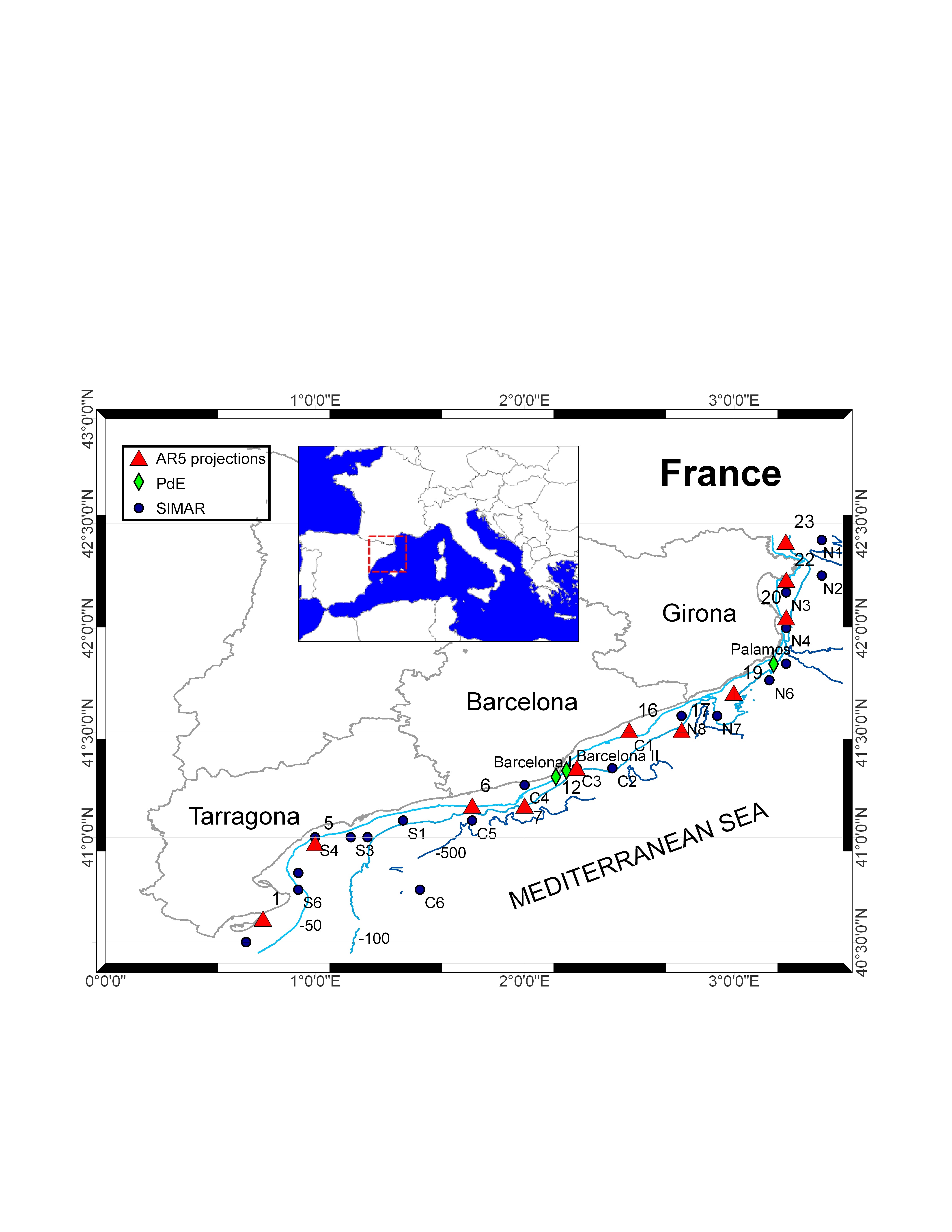 Figure 1
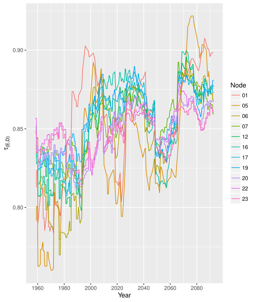 Figure 10
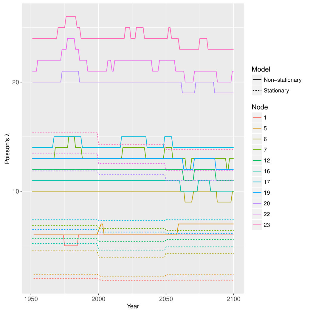 Figure 11
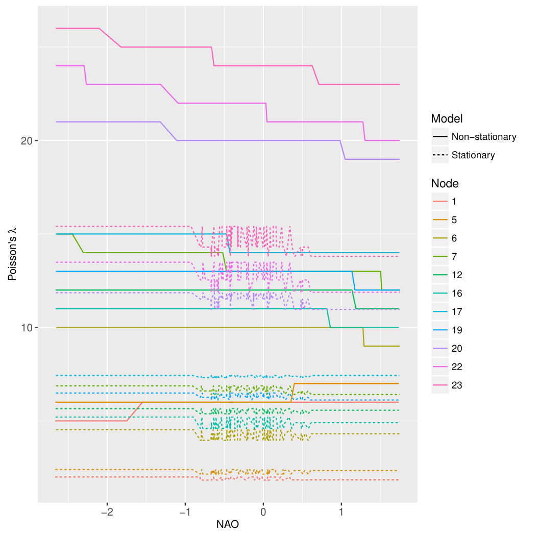 Figure 12
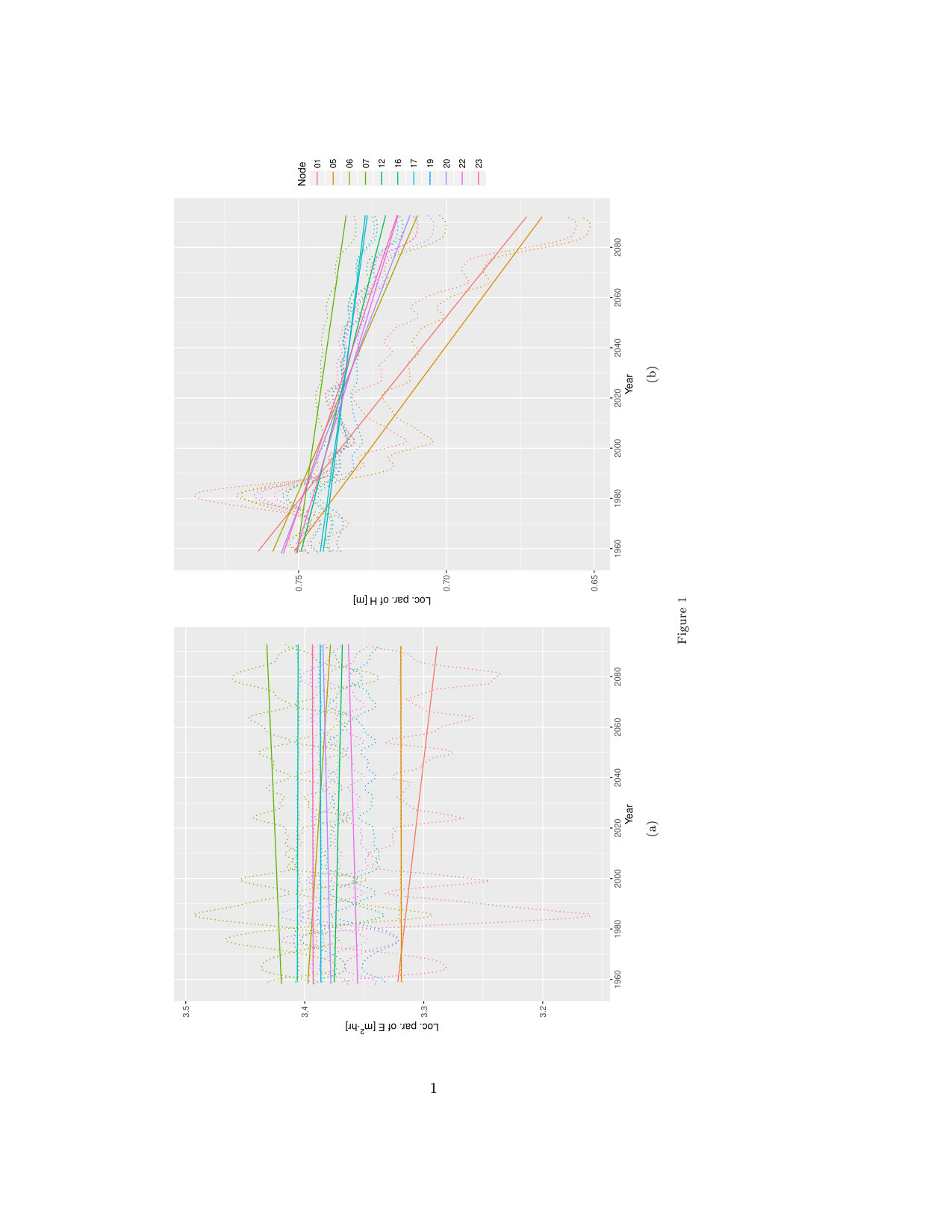 Figure 13
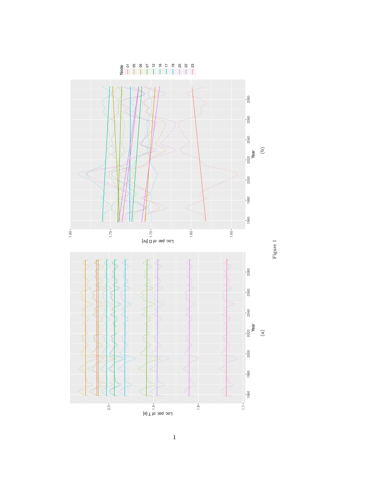 Figure 14
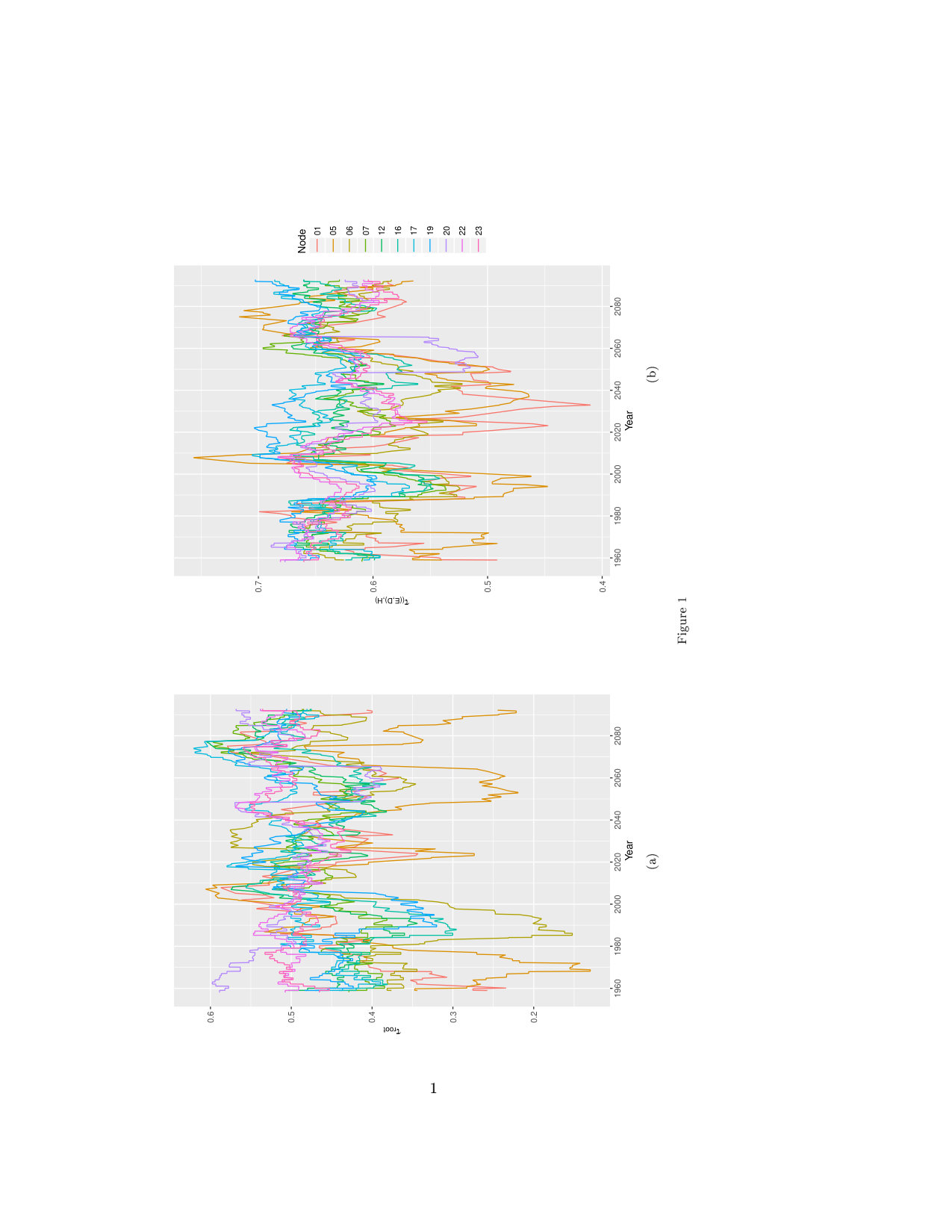 Figure 15
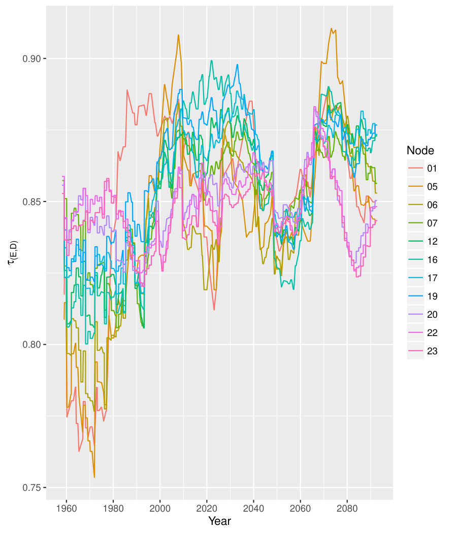 Figure 16
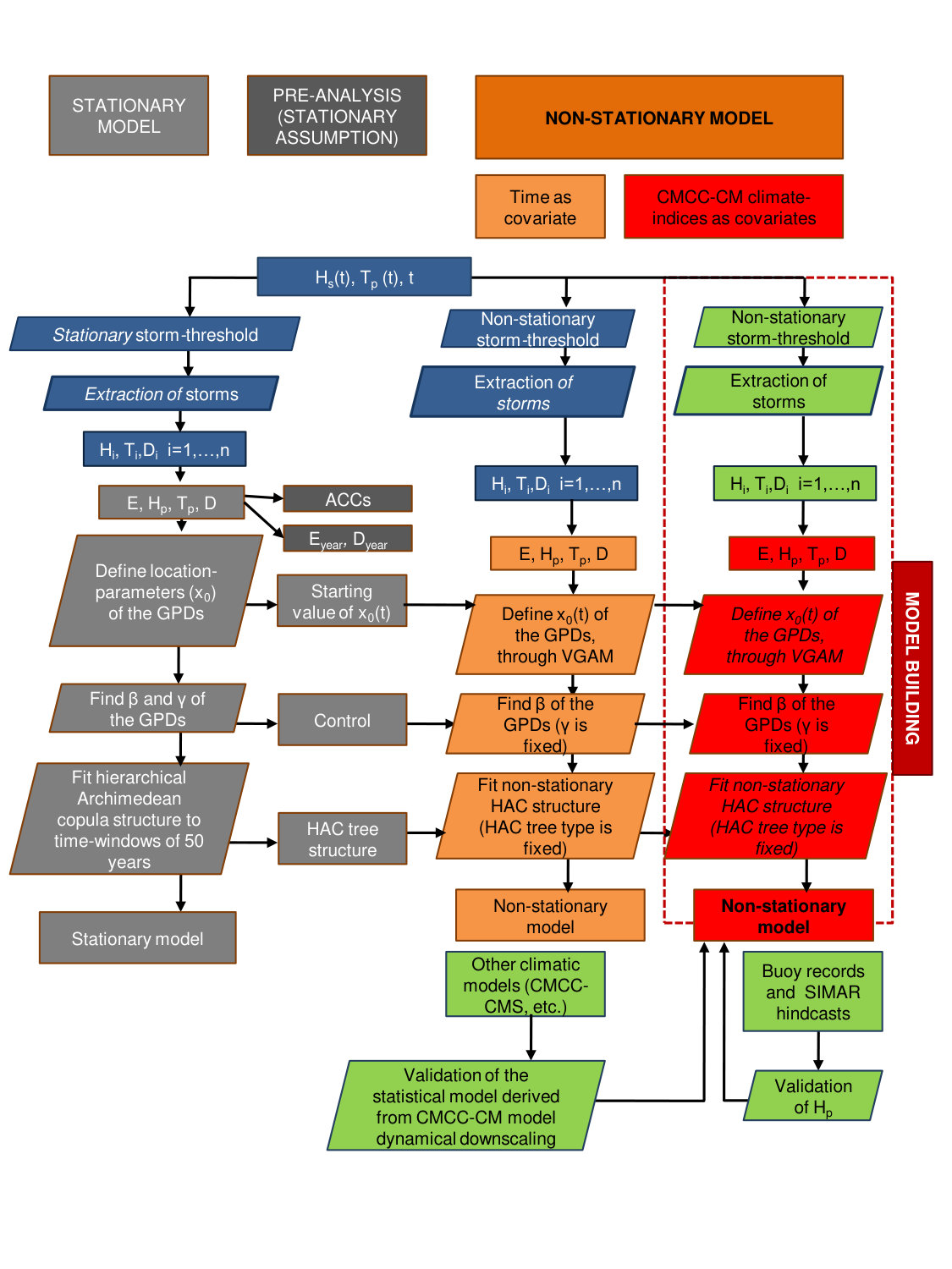 Figure 2
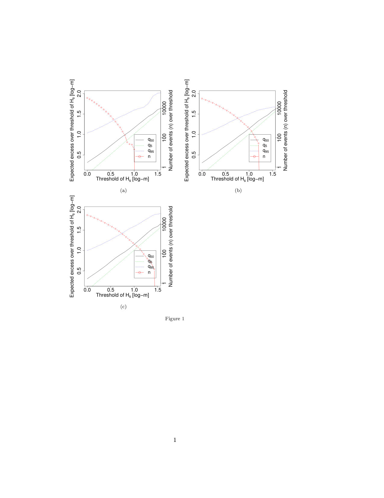 Figure 3
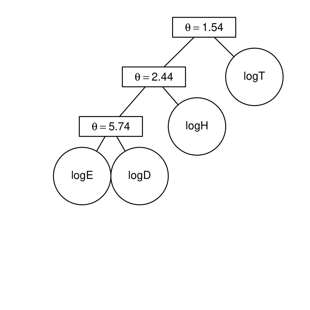 Figure 4
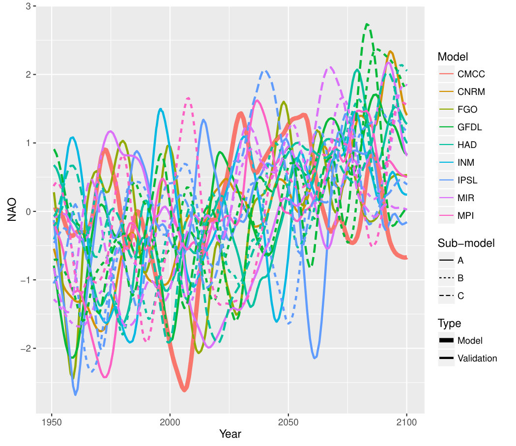 Figure 5
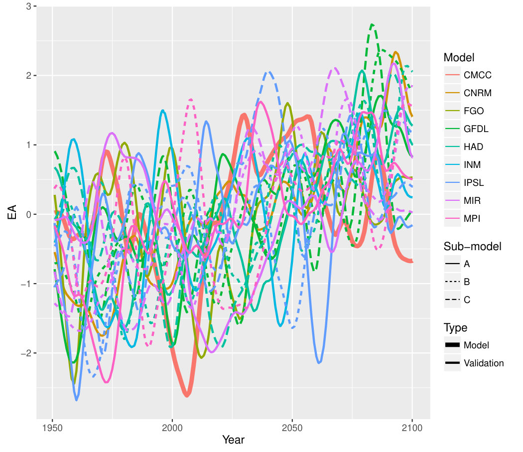 Figure 6
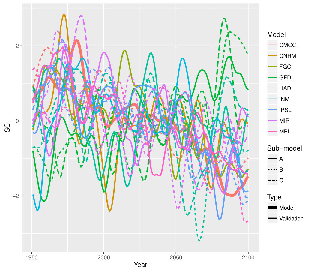 Figure 7
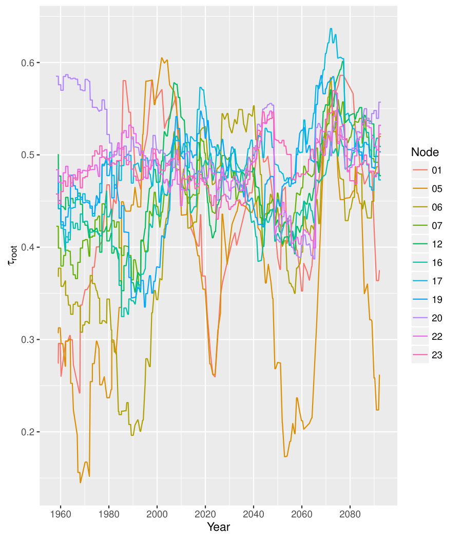 Figure 8
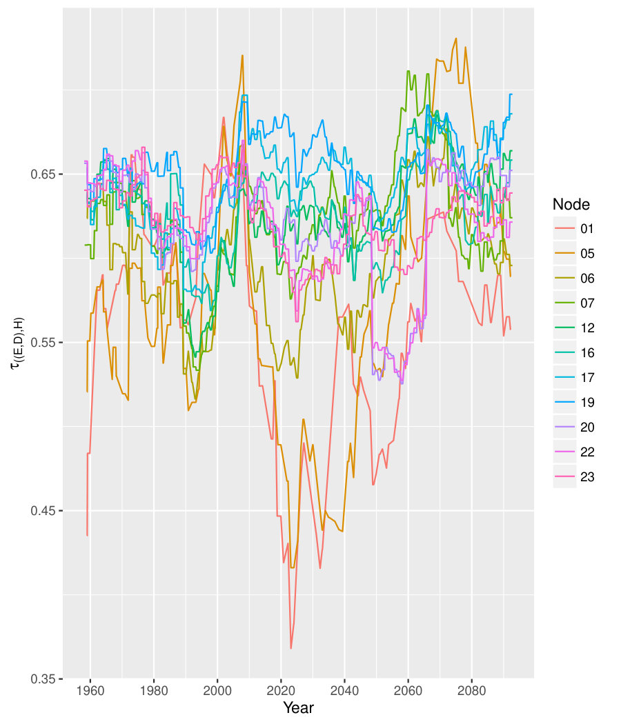 Figure 9
| Acronym | Global circulation-model | Latitude | Longitude |
| grid size (∘) | grid size(∘) | ||
| CMCC_A | CMCC-CM | 0.7484 | 0.75 |
| CMCC_B | CMCC-CMS | 3.7111 | 3.75 |
| CNRM_A | CNRM-CM5 | 1.4008 | 1.40625 |
| FGO_A | FGOALS-G2 | 2.7906 | 2.8125 |
| GFDL_A | GFDL-CM3 | 2 | 2.5 |
| GFDL_B | GFDL-ESM2G | 2.0225 | 2 |
| GFDL_C | GFDL-ESM2M | 2.0225 | 2.5 |
| HAD_A | HadGEM2-AO | 1.25 | 1.875 |
| HAD_B | HadGEM2-CC | 1.25 | 1.875 |
| HAD_C | HadGEM2-ES | 1.25 | 1.875 |
| INM_A | INM-CM4 | 1.5 | 2 |
| IPSL_A | IPSL-CM5A-LR | 1.8947 | 3.75 |
| IPSL_B | IPSL-CM5B-LR | 1.8947 | 3.75 |
| IPSL_C | IPSL-CM5A-MR | 1.2676 | 2.5 |
| MIR_A | MIROC-ESM | 2.7906 | 2.8125 |
| MIR_B | MIROC-ESM-CHEM | 2.7906 | 2.8125 |
| MIR_C | MIROC5 | 1.4008 | 1.40625 |
| MPI_A | MPI-ESM-LR | 1.8653 | 1.875 |
| MPI_B | MPI-ESM-MR | 1.8653 | 1.875 |
| SIMAR/buoy | AR5 | Ait.dist() | KL.dist() |
|---|---|---|---|
| node | node | (Aitchison distance) | (Kulback-Leibler distance) |
| N1 | 23 | 0.52 | 0.07 |
| N3 | 22 | 0.81 | 0.16 |
| N4 | 20 | 0.18 | 0.01 |
| N7 | 19 | 0.45 | 0.05 |
| N8 | 17 | 0.54 | 0.07 |
| C1 | 16 | 0.20 | 0.01 |
| C3 | 12 | 0.26 | 0.02 |
| C4 | 07 | 0.26 | 0.02 |
| C5 | 06 | 0.96 | 0.24 |
| S4 | 5 | 1.31 | 0.30 |
| S7 | 1 | 0.98 | 0.23 |
| PdE-Begur | 20 | 0.96 | 0.24 |
| PdE-BCN-I | 12 | 1.31 | 0.41 |
Peer Reviews
No public reviews on file for this paper yet. If you reviewed it on a platform where reviews are public (OpenReview, ICLR, NeurIPS, ICML), you can paste yours below so the community can read it here.
Videos
No videos yet. Explain this paper in a talk, walkthrough, or lecture? Add one.
Multivariate statistical modelling of future marine storms
J. Lin-Ye11footnotemark: 1
M. García-León
V. Gràcia
M.I. Ortego
P. Lionello
A. Sánchez-Arcilla
Laboratory of Maritime Engineering, Barcelona Tech, D1 Campus Nord, Jordi Girona 1-3, 08034, Barcelona, Spain
Department of Civil and Environmental Engineering, Barcelona Tech, C2 Campus Nord, Jordi Girona 1-3, 08034, Barcelona, Spain
Centro Euro-Mediterraneo sui Cambiamenti Climatici, Via Augusto Imperatore, 16, Lecce, Italy
Abstract
Extreme events, such as wave-storms, need to be characterized for coastal infrastructure design purposes. Such description should contain information on both the univariate behaviour and the joint-dependence of storm-variables. These two aspects have been here addressed through generalized Pareto distributions and hierarchical Archimedean copulas. A non-stationary model has been used to highlight the relationship between these extreme events and non-stationary climate. It has been applied to a Representative Concentration pathway 8.5 Climate-Change scenario, for a fetch-limited environment (Catalan Coast). In the non-stationary model, all considered variables decrease in time, except for storm-duration at the northern part of the Catalan Coast. The joint distribution of storm variables presents cyclical fluctuations, with a stronger influence of climate dynamics than of climate itself.
keywords:
wave storm , Catalan Coast , hierarchical Archimedean copula , generalized Pareto distribution, non-stationarity, generalized additive model
††journal: Applied ocean research
1 Introduction
Extreme events characterization is a key piece of information for an efficient design and construction of any coastal infrastructure. Natural extreme events, such as hurricanes, tsunamis or earthquakes, can lead to considerable economic losses (Shi et al., 2016). From all these hazards, marine storms cause most of the damage to non-seismic coasts. This situation may eventually be aggravated as a consequence of Climate-Change, which affects the intensity and frequency of extreme wave-conditions (Wang et al., 2015; Hemer and Trenham, 2016).
Changes in climate can affect several coastal hazards: flooding (Hinkel et al., 2014; Wahl et al., 2016), erosion (Hinkel et al., 2013; Casas-Prat et al., 2016; Li et al., 2014), harbour agitation (Sánchez-Arcilla et al., 2016; Sierra et al., 2015) and overtopping (Sierra et al., 2016). A robust statistical characterization of storms is, thus, required to assess coastal risks and to forecast storm impacts (Sánchez-Arcilla et al., 2014; Gràcia et al., 2013). The stationary climate assumption, common approach in the last decades for designing infrastructures, does no longer hold valid in a context of Climate-Change. Hence, there is a pressing urge for methodologies that consider non-stationarity, not only in trends, but also in higher statistical moments such as variance.
Usual statistical distributions for extremes such as the Generalized Pareto Distribution (GPD) or the Generalized Extreme Value distribution have three parameters: location, scale and shape. Rigby and Stasinopoulos (2005) proposed a generalized additive model for these three parameters to predict river flow-data from temperature and precipitation on the Vatnsdalsa river (Iceland). Yee and Stephenson (2007) developed a methodology that allows extreme value distributions to be modelled as linear or smooth functions of covariates. One of the examples they presented was the modelling of rainfall in Southwest England. Du et al. (2015) carried out frequency analyses using meteorological variables, where they tested several combinations of co-variates with generalized additive models for location, scale and shape, and concluded that meteorological co-variates improve the characterization of non-stationary return periods. Méndez et al. (2007) used a time-dependent generalized extreme value distribution to fit monthly maxima series of a large historical tidal gauge record, allowing for the identification and estimation of time scale such as seasonality and interdecadal variability. Méndez et al. (2008) extended the former methodology to significant wave-height, while considering the effect of storm duration.
For design purposes, the most analysed variable in marine storms is the significant wave height (), usually considered to be independent from other wave storm-components such as peak-period (), or storm-duration (). Nevertheless, these variables are known to be semi-dependent (De Michele et al., 2007). Univariate analyses on singular variables, such as , cannot thus describe coastal processes adequately (Salvadori et al., 2014), leading to misestimation of coastal impacts and risks.
The relationship among storm variables can be modelled with statistical techniques such as parametric probability distributions (Ferreira and Soares, 2002), asymptotic theory (Zachary et al., 1998), joint modelling (Bitner-Gregersen, 2015), or copulas (Genest and Favre, 2007; Trivedi and Zimmer, 2007), among other techniques. Copulas were proposed by Sklar (1959), and have recently attracted attention from coastal engineers (Corbella and Stretch, 2012; Salvadori et al., 2015). Wahl et al. (2011) applied fully nested Archimedean copulas to wave storms off the German coast. They first characterized the highest energy point and its intensity and then incorporated the significant wave height. Complementary to these methodologies, Gómez et al. (2016) has implemented a time varying copula to analyse the relationship between air temperature and glacier discharge, which is non-constant and non-linear through time. In this case, both marginal and copula parameters depend on time, and a full Bayesian inference has been applied to obtain these parameters.
Based on this, the present work characterizes the extreme wave climate under a Representative Concentration Pathway 8.5 Climate-Change scenario (RCP8.5, i.e. an increase of the radiative forcing values by year 2100 relative to pre-industrial values of ; Stocker et al. (2013)) for a fetch-limited environment (Catalan coast). The study is based on a set of geographical nodes which are equidistant along the Catalan coast. Only eleven nodes out of the total twenty-three are used in this paper, since they represent well the main features and spatial variability of the storm distributions (see Fig. 1, red triangles). Two of the eleven nodes are in intermediate waters, while the rest are in deep waters. The subsequent analysis is performed assuming, first, stationary, and then, transient conditions.
Section 3 describes the methodology and the theoretical background. Section 2 presents the study area. Section 4 lists main results, which are discussed in Section 5. The conclusions are summarized in Section 6.
2 Study area
The Mediterranean Sea (see Fig. 1) is a semienclosed basin, constrained by the European, Asian and African continents. It has a narrow connection to the Atlantic Ocean (Gibraltar Strait), as well as an access to the Black Sea. In terms of waves, the Mediterranean Sea can be splitted into different partitions (Lionello and Sanna, 2005). This paper deals with the Catalan coast, which can be found at the northwestern Mediterranean sector. This area has, as its main morphological features, a) mountain chains which run parallel and adjacent to the coast, b) Pyrenees Mountains to the north, and c) the Ebre river valley to the south. These orographic discontinuities, along with the major river valleys, serve as channels for the strong winds that flow towards the coast (Grifoll et al., 2015).
The most frequent and intense wind in the Catalan Coast is the Tramuntana (north), appearing in cold seasons. It is the major forcing for the northern and central Catalan Coast waves. However, from latitude southward, the principal wind direction is the Mistral (northwest), which is formed by the winds that flow downhill the Pirinees or between the gaps of the mentioned mountains. A secondary wind, the Ponent (west), comes from the depressions in northern Europe. It is the second most frequent one, with limited intensity. Eastern winds are the ones with larger fetch for intense sheer stress, corresponding to low pressure centres over the northwestern Mediterranean. During the summer, there are southern sea-breezes and estern winds, triggered by an intense high-pressure area on the British Islands.
The northwestern Mediterranean Sea is a fetch-limited environment, primarily driven by wind-sea waves (Bolaños et al., 2009; Sánchez-Arcilla et al., 2016). The distance that waves travel, from the storm genesis to the Catalan Coast, is at most one-sixth that of a wave that reaches the Atlantic European coasts (García et al., 1993). Therefore, the corresponding wave-periods, in the northwestern Mediterranean, are much shorter.
The present climate presents a mean significant wave height of from Barcelona City nortward, and southward. Maximum ranges between in the southern coast to at the northern coast (Sánchez-Arcilla et al., 2008; Bolaños et al., 2009). Casas-Prat and Sierra (2013) projected future wave climate at the Catalan Coast through Regional Circulation Model outputs from the A1B scenario (IPCC, 2000) for the time-period comprising 2071-2100. Their results showed a variation compared to present of the significant wave height around , whereas the same variable for a return-period exhibits rates around .
3 Proposed methodology
The methodology here developed leads to a robust assessment of storm pressures under present or future climates. Regional projections are obtained from a deterministic approach, based on the underlying physics, avoiding the computationally expensive dynamical downscaling and the oversimplification of conventional empirical downscaling. Wave storms are first characterized assuming stationarity (see Fig. 2). From here, the joint probability structure is derived and this will serve as a basis for the non-stationary model of the selected projection (in this case, under the RCP 8.5 scenario). A non-stationary model is then built, and constitutes the main part of the proposed methodology, described below.
3.1 Data and storm components
The analysis has been performed considering the wave-climate at the Catalan Coast under a RCP 8.5 Climate-Change scenario. This scenario considers a concentration in the atmosphere close to in 2100, which is double that of any other scenario in the Fifth Assessment Report (Stocker et al., 2013). The modelling chain comprises the CMCC-CM (Scoccimarro et al., 2011) Global Circulation Model (see Table 1), providing boundary conditions for the Regional Circulation Model COSMO-CLM (Rockel et al., 2008). The statistical model derived from the CMCC-CM dynamical downscaling has been validated with a total of eighteen Global Circulation Models, shown in Table 1. This list includes models from the same experiment (CMIP5, Taylor et al. (2012)) and from the same Climate-Change-scenario (RCP 8.5), covering, thus, a comprehensive range of predictors. The COSMO-CLM grid, that has a resolution of , spans the whole Mediterranean region. The next step consists of the WAM (WAMDI Group et al., 1988) wave model, where the just mentioned wind fields serve as an input, for the same domain and spatial resolution. The projections considered in all three models (Global Circulation Model, Regional Circulation Model and WAM), span the interval from year 1950 to 2100.
The nodes considered for the AR5 projections and subsequent analyses (Fig. 1, red triangles) are combined with buoy and SIMAR (Gomez and Carretero, 2005) hindcast points (green rhombuses and black dots, respectively) for validation purposes. All selected nodes (except 1 and 16) are located in deep waters, and thus the WAM model is a suitable option (Larsén et al., 2015). The application of this code to nodes 1 and 16, in intermediate waters, may present certain limitations and would, thus, require further exploration and research. The validation dataset comes from SIMAR hindcasts and Puertos-del-Estado buoy records, corresponding to the period 1990 to 2014. Storms here are clustered into storm-years. Storm-years (called “years”, hereafter), which are periods of 12 months, from July to June of the next year.
Four main variables have been selected to describe the storm-intensity conditions: storm energy (), significant wave-height at the storm-peak (), peak wave-period at the storm-peak (), and duration (). The and are aggregated parameters, related to the total impact of the storm, whereas and represent the maximum intensity of the event. , , and take positive real values and, consequently, they have been log-transformed to avoid scale effects (Egozcue et al., 2006).
3.2 Pre-analysis (stationarity assumption)
Prior to the actual modelling, an explanatory analysis has been carried out with the available wave data. A set of stationary models has been built by selecting equidistant time slices from the total sample, following previous work by other authors with similar hydrodynamic variables (Muis et al., 2016; Vousdoukas et al., 2016). The three time-frames are labelled as: (i) past (PT,1950-2000); (ii) present-near-future (PRNF, 2001-2050), and far future (FF, 2051-2100). Storms have been defined using a stationary threshold of significant wave-height, based on previous work (Lin-Ye et al., 2016). Although the time period in Lin-Ye et al. (2016) is significantly shorter than in the present paper, this threshold should be acceptable for the three time-frames as it falls on the linear part of the excess-over-threshold plot (Fig. 3), according to methodology previously developed by Tolosana-Delgado et al. (2010).
The next step of the pre-analysis consisted in building dependograms of the selected storm variables, which were then visually inspected for non-stationary behaviour. Each variable is also presented in absolute concentration curves (ACC), where ACC1 indicates the ratio of at a given time-frame, to the one in the PT inteval (Yitzhaki and Olkin, 1991). ACC2 denotes the same ratio, but with . Thus, ACC1 represents on changes in the mean, whereas ACC2 reflects on the evolution of the variance. This analysis has been performed for the energy and duration of the total events of a storm-year, and , as well as the mean and of a storm-year, and , to assess non-stationary trends.
3.3 Stationary model
The probability distribution of each storm variable is fit by a GPD. Being the excess of a magnitude over a location-parameter , conditioned to , the support of is (Coles, 2001). is the upper bound of the GPD. The GPD cumulative function is, then,
[TABLE]
where is the scale parameter and is the shape parameter. As a first approximation, the values of the location parameters obtained in Lin-Ye et al. (2016) have also been used in this case. The departure from these values is described in Sub-section 4.2.
The Hierarchical Archimedean copula (HAC) is a flexible tool that describes the dependence between variables via the nesting of a subset of -D copulas (Sklar, 1959; Nelsen, 2007; Okhrin et al., 2013). The Gumbel type HAC with a mean aggregation method is selected for this case of extreme events, according to Lin-Ye et al. (2016). A -dimensional Archimedean copula has the form
[TABLE]
for a given generator function . A Gumbel generator has been selected since it defines the dependence in the upper tail of the probability distribution. Note that a family of asymmetric copulas (Vanem, 2016) would include physical limitations, such as wave steepness, where high cannot commute with large . Due to the complexity of non-stationarity, the asymmetric copulas must be carefully introduced in a more mature future version of the proposed model.
The HAC aggregates the Gumbel generator parameters using a series of coefficients called , which can be transformed to Kendall’s (Kendall, 1937; Salvadori et al., 2011). denotes independence when , and total dependence when tends to . The goodness-of-fit of the HACs at each time-frame has been assessed by using goodness-of-fit plots of the empirical copulas (Lin-Ye et al., 2016). The statistic (Gan et al. (1991)) serves to quantify the goodness-of-fit. It takes values in , and a perfect fit happens when . According to our experience in the Catalan Coast, the HAC-structure in Fig. 4 should be applicable to this area. There is another approach for events where is less inter-dependent with and (Lin-Ye et al., 2016), but this type of structure is of less interest in this study, as will be discussed later. The nesting levels in Fig. 4 start at the branching of the tree-like structure, and end at the top "root" level.
3.4 Non-stationary model
Extreme events are scarce by nature. The shorter the time-window considered, the smaller will be the available information, with larger uncertainty. This assumption means that, for the time-windows of considered in the stationary model, there are fewer samples of high extreme events. Hence, the probability distribution function’s upper tail estimation would not provide results reliable enough. Previous studies indicate that Climate-Change also has a non-negligible effect on extremes (Trenberth and Shepherd, 2015; Hemer and Trenham, 2016; Du et al., 2015), so assumptions such as a stationary storm-threshold cannot be adopted. This is a first indication that non-stationarity needs to be addressed (Vanem, 2015).
In the non-stationary model, vectorial generalized additive models (VGAM, Yee and Wild (1996)) have been used to determine storminess, storm-thresholds and GPD parameters (Rigby and Stasinopoulos, 2005; Yee and Stephenson, 2007). The VGAM consists of a linear function (Fessler, 1991; Hastie and Tibshirani, 1990):
[TABLE]
where is the dependent variable, is the independent variable that generates . is a sum of smooth functions of the individual covariates and . In this case, is not the scale parameter of the GPD. Additive models do all the smoothing in , avoiding the large bias introduced in defining areas in .
The mathematical assumptions for regression models are: 1) incorrelation, 2) normality, and 3) homoscedasticity of residuals. Assumption 1) is assessed with a ACF plot, assumption 2) can be assessed with a Q-Q plot against a distribution, where the sample standard deviation is used as . Assumption 3) can be analysed on a graph of fitted value vs. residuals. When the predicted variable is a counting one, a vectorial generalized linear model (VGLM) can be adopted (Yee and Wild, 1996). The VGLM is a particular case of VGAM. The storminess is a counting variable, and its relationship with any other factor can be approximated by a Poisson distribution.
The storm-threshold is then estimated through a VGAM that approximates its relationship with a factor by a Laplace distribution. Once storms are selected, their non-stationary GPD location-parameter is estimated through quantile regression (Koenker, 2005). The quantile regression is a specific type of VGAM, and it estimates the conditional quantile of a response variable as a function of covariates . The equation must then be minimized, where for residuals . is a roughness coefficient that controls the trade-off between quality of fit to the data and roughness of the regression function; and is a roughness penalty (Northrop and Jonathan, 2011; Jonathan et al., 2013). The above mentioned has nothing to do with the of Kendall. Regarding the rest of the GPD parameters: is assumed to remain constant; is considered to depend on co-variates, and is estimated with VGLMs.
The option of using time as a covariate is examined in the non-stationary model, just to assess the evolution of other variables. The predicting function is a -degree spline (Hastie and Tibshirani, 1990). Alternative predictive parameters seems to present a greater potential. Climate-indices are eligible candidates (Rigby and Stasinopoulos, 2005), for which the linear interpolation function has been selected, advocating the principle of parsimony. Possible climate-indices are the North Atlantic Oscillation (NAO, Hurrell and Deser (2009)), the Easterly Atlantic index (EA, Barnston and Livezey (1987)), the Scandinavian oscillation (SC, Barnston and Livezey (1987)), and their first and second time derivatives. These climate-indices have been scaled to have a mean value equal to zero and a variance equal to unity, and they actually introduce time as an implicit covariate. They were computed from the monthly-averaged sea level pressure fields, from the global circulation-model listed in Table 1. In order to avoid sudden oscillations that would hinder interpretation, the time series of climate-indices have been filtered with a order lowpass Butterworth filter (Butterworth, 1930), whose low-pass period was of .
Different results among global circulation-models should be expected, despite the same post-processing treatment for all of them. The grid-size and physical implementations are not the same, the model with the highest resolution () is CMCC-CM, which is the one that has served as the calibration model. There are also slight divergences on how the model addresses the evolution of emissions (Friedlingstein et al., 2014).
Once storms events have been selected, , , and can be extracted. The effect of climate-indices as covariates is assessed at nodes 7 and 21, as these nodes represent the most distinct spatial patterns (see Sec. 2 and Fig. 1). The goodness-of-fit of the resulting VGAM with different combinations of covariates is contrasted with a likelihood-ratio test (LRT, Vuong (1989)), the Akaike information criterion (AIC, Akaike (1987)) and the Bayesian information criterion (BIC, Tamura et al. (1991)). A censorship analysis is carried out on the sample for these two nodes, corresponding to two subsets of GPDs for: a) onshore winds and b) offshore winds. For the two samples in the censorship analysis, and for the combined sample, the proposed model is calibrated with climate-indices derived from the CMCC-CM global circulation-model. The climate-indices from the other eighteen models (Figs. 5, 6, and 7) serve to predict what would be the probability distribution functions under a wide range of plausible values. In the results and discussion section, the quantile, a common quantile for hazard and design (Goda, 2010), has been used to inter compare these.
VGAM uses, thus, global circulation climate-indices as covariates to create time series of quantiles. A way of quantifying how these time series differ from the baseline (CMCC-CM), is by computing the Euclidean distance between the estimated partial autocorrelation coefficients of each time series (Galeano and Peña (2000)). This metric takes values in , being [math] the shortest distance (i.e. closer similarity between models), and , the largest one.
Regarding the joint dependence structure of the proposed model, storms are clustered into periods of , under the assumption that there is stationarity in these . Because of the persistence of the climate-indices considered, this is a plausible hypothesis. are also the shortest time-span that provides a sufficient number of storms to determine the HAC structure. Larger time-windows would offer a greater number of storms, but with a non-stationary dependence parameter. Non-stationary HAC dependence parameters are obtained at each node, for this moving time-window of . Each time-window overlaps with the former and the following ones, in half-a-year, to characterize the non-stationary effect.
The Gumbel HAC dependence structure from the stationary-model is also used in the non-stationary model. Particularly, the HAC-structure in Fig. 4 is adopted for the whole non-stationary model. The fitting criteria is the Maximum Likelihood method, where the HAC-structure in the stationary-model (see sub-section 3.3) is set as the unique structure for all nodes and for the whole simulation period. The selection of only one HAC-structure follows the principle of parsimony, being this HAC the one that better characterizes the joint-dependence at most spatial nodes during the three time-frames of the stationary model.
The Kwiatkowski-Phillips-Schmidt-Shin (KPSS) test (Kwiatkowski et al., 1992) is applied to the dependence-parameters of the HAC, to look into the stationarity of the time series. The p-value of such test gives the level of significance at which the null test cannot be rejected. In other words, on how likely the dependence-parameter is actually stationary.
To represent projected climatology, the probability distribution function of the should resemble that of observed storm conditions (from buoys and hindcasts). The proposed model has been validated at the nodes listed on Table 2 (see Figs. 1 for node location), as follows. The SIMAR/buoy data validation nodes are denoted:
[TABLE]
and the model data (written as , here)
[TABLE]
They are next combined to form a joint dataset:
[TABLE]
Such set is partitioned into four intervals, separated by the quartiles . There are elements from both SIMAR/buoy and AR5 projections, in each interval. The quartiles are selected as boundaries because buoy records are often interrupted due to harsh wave conditions. Then, if the selected intervals are too small, some of them might be empty, which would lead to indetermination of the distance between model and data.
Two vectors are defined as
[TABLE]
and
[TABLE]
where is the vector for observations, and is the one for projections. Each element of the vector is the summation between two quantiles of the probability distribution function. Therefore, and are compositional data, their elements being parts of a whole (Egozcue and Pawlowsky-Glahn, 2011), and fulfilling some other properties defined in Aitchison (1982) and Egozcue et al. (2003). The distance between these two vectors can be determined with an Aitchison measure (Aitchison, 1992; Pawlowsky-Glahn and Egozcue, 2001),
[TABLE]
Where and are two compared vectors. Another measure for the distance is the Kullback-Leibler divergence (Kullback, 1997)
[TABLE]
This function measures the extra entropy of the probability distribution of the model, with respect to the probability distribution of the observations. Note that for any , , must imply , to avoid indertemination, thus ensuring that the model considers all the values that the observations show. Also, whenever , the contribution of the -th term is null, as .
Both eq. 8 and 9 are distances, and thus take values in . The module of the vector is a particular case of both distances (Egozcue and Pawlowsky-Glahn, 2011), and thus both can be compared to the vectorial module, in Euclidean space, of and , which should be of order .
4 Results
4.1 Pre-analysis (stationarity assumption)
The dependograms, which do not vary for the different time-frames, show inter-dependence of and the other variables (, , ), except at node 1 in the FF. ACC1 and ACC2 ratios are represented in Figs. 1 to 3 of the Supplementary material. and decrease in PRNF and FF (see Supplementary material, Fig. 1). , , and are equal to one for the entire Catalan Coast (figures not shown). is slightly below 1, being specially low in bays or similar local coastal domains. is approximately 1.05 in the northern sector (Girona). and are high in apexes like the Creus cape (near node 22), and low in bays like the Tarragona one (see Fig. 1). All the ACC2 ratios are slightly below one in the PRNF (see Supplementary material, Fig. 2), and get closer to one in the FF (see Supplementary material, Fig 3). The temporal evolution of , , and are presented in Figs. 4 to 7 of the Supplementary material. The are only autocorrelated at node 22 and 12, with a lag of in PT, and are not autocorrelated for larger lags. is autocorrelated at nodes 6, 12, 16, 17, 20, 22 and 23, at different time-frames, and is autocorrelated along the entire Catalan coast. is autocorrelated at node 22, in PT, with a lag of , and at node 1 in PRNF, with a lag of .
4.2 Stationary model
After defining the GPD parameters and , each storm-intensity variable is fit by a GPD, of discontinuous support. has required an increase of its location-parameter ( in FF, at nodes 20 and 22), before fitting GPD. Depending on location, differences may appear within storm-parameters, possibly due to wave propagation effects and the control of land winds at the northermost and southernmost sectors. Unlike for SIMAR hindcasts, the HAC-structure in Fig. 4 is the only one present at all nodes and for all time-frames. The goodness-of-fit of the HAC are represented in Figs. 8 to 10 of the Supplementary material. The parameter and the graph show a good fit of the Gumbel-HAC, as observed in Lin-Ye et al. (2016).
4.3 Non-stationary model
Two different kinds of non-stationary model have been built: a) using time as the single covariate (NS-T hereafter); and b) implementing large scale climate-indices as covariates (NS-CI hereafter). By using time alone as a covariate to storminess, the storm threshold and GPD parameters, whenever NS-T shows a clear time-dependent behaviour, the non-stationary model NS-CI is applicable. Figures 8, 9, and 10 show the temporal evolution of the HAC dependence-parameters for NS-T. The KPSS test (Kwiatkowski et al., 1992) is applied on for the NS-T model, and the outcome is that the null hypothesis of stationarity cannot be rejected in of the cases. That is, is highly non-stationary.
Regarding storminess, the SIMAR-dataset and the available buoy-records confirm higher storminess-indices () at the northern coast (Figs. 11 and 12). Figure 11 shows that decreases with time, but the stationary model can only capture this trend via the predefined time-blocks. This supports using a non-stationary model to improve the representation of the extreme wave-climate. A sensitivity analysis has been carried out on the covariates, at nodes 7 and 21. In the censorship analysis within this sensitivity analysis, the subset with on-shore winds has presented better fit with NAO as covariate, whereas the subset with offshore-winds has done the same with SC. However, an additional test on the rest of nodes has not shown better performance, and for the sake of consistency and parsimony, the uncensored sample has been applied in all nodes. In the uncensored sample, the maximum likelihood estimation indices are smallest for NAO and SC, meaning that these are the covariates that mostly influence . The LRT, in turn, denotes that the combination of the two do not provide significantly more information than each of these factors by themselves. What is more, the AIC and the BIC are lowest for the NAO. Therefore, the NAO is selected as the sole covariate for the Poisson-VGAM. Figure 12 shows that increases with negative NAO.
NAO, EA, SC (see Figs. 5, 6, and 7) and their first and second derivatives are also used as covariates in the NS-CI VGAM to predict the storm-thresholds and the GPD parameters. The normality and homoscedasticity assumptions of the VGAM (Rigby and Stasinopoulos, 2005) cannot be rejected for the storm-threshold and the GPD parameters and . The incorrelation assumption is similarly not rejected for the GPD parameters and , but should be rejected for the storm-threshold. The latter non-conformity should be considered when examining the final results.
The statistical model derived from the CMCC-CM (CMCC-A) global circulation-model is, then, compared to the eighteen other models, in the Supplementary material, Figs. 11 to 18 show the similarity of CMCC-CM results to other global circulation-models. For nodes 7 through 23, the distance between each pair of climate-index models is relatively short for most cases, except MIROC-ESM-CHEM (MIR-B) and MIROC5 (MIR-C). The Aitchison and the Kullback-Leibler distances between and are shown on Table 2. The location-parameters of the GPD are presented in Figs. Multivariate statistical modelling of future marine storms and Multivariate statistical modelling of future marine storms. from the NS-CI HAC-structures are presented in Figs. Multivariate statistical modelling of future marine storms a 13.
5 Discussion
5.1 Pre-analysis (stationarity assumption)
The decrease in and denote loss of energy and duration of storms in future climates. presents more drastic temporal changes in the northern Catalan Coast. The increase in the FF, faster than in the PRNF, suggesting that storm-components will present a larger variance over time. does not behave like . Possibly, has a certain role in lowering the variance of . The northward decrease in variance of , observed in Figs. 2 and 3 of the Supplementary material, was also reported for SIMAR hindcasts, in Lin-Ye et al. (2016). This phenomenon occurs when depends heavily on fetch and origin, rather than being a function of wind pulse characteristics.
As for , , and (see Supplementary material, Figs. 4 to 7), and fluctuate from PRNF on, whereas they have been considerably stationary in PT (see Supplementary material, Fig. 4 and 5). The general trend in is a high in the first quarter of the XXIst century, followed by approximately of low , and another quarter of century of high . has a cyclicity of approximately . has the same cyclicity as , but it presents stationarity in the PRNF, instead of presenting it in the PT. The time derivatives, , , , fluctuate periodically, but no clear cycles are detectable (not shown here). The reasons behind the clusterings of , , and peaks need further atmospheric analysis (see Sub-section 5.3), but the consequences can be outlined.
, behaves similarly to . becomes less stable from PRNF onward. and behave similarly, due to the definition of , which includes . The low and the high at the Ebre-Delta in the midst of the XXIst century may lead to more sediment mobility and a loss of resilience of the area, which is already highly erosive (CIIRC, 2010). The fact that depends more on a summation of small storms than a great one elevates the importance of the smaller storms with to of return period. Low lifetime solutions such as Transient Defence Measures (Sánchez-Arcilla et al., 2016) would be a plausible solution for these periods. What can be expected is that these two seasonal features are not going to be as predictable in the PRNF and FF as in PT, but there are some remarkable periods in the second half of the XXIst century, when extreme events are present. From the fluctuations of , , and , it can be perceived that a non-stationary approximation is needed.
5.2 Stationary model
The fact that the HAC-structure in Fig. 4 is predominant in the AR5-projections might be due to being more dependent of - in these AR5 projections than in the SIMAR hindcasts (Lin-Ye et al., 2016). This means a remarkable difference between AR5 and SIMAR data. Apparently, the AR5 waves have a lower variability on than the SIMAR data, thus leading to this phenomenon. and are averaged values, and a higher correlation can be expected with data that have lower variability values. In other words, SIMAR data might be more heteroschedastic than AR5 data, and this affects the copula definition. Here, the goodness-of-fit of the Gumbel-type HAC with a “mean”-type aggregation-method should be acceptable (see Supplementary material, Figs. 8 to 10).
The dependence of with the subset - increases southward due to the proximity of node 1 to the coast (see Fig. 1). The fact that , and have milder values in south-Barcelona and in Tarragona (not shown here), indicate that storms in the south are less energetic and durable than at northern locations. Also, and is the strongest related components in all storms, so the more energy a storm has, the more time it needs to be dissipated, as expected.
becomes independent from the rest of the variables (, and ) in the FF. It is observed that, at nodes 1 and 2, , and decrease in the second half of the XXIst century. However, the time series of does not present any trend. Also, except , the rest of the variables consistently depend on ; as decreases in the second half of the XXIst century, the other variables behave in the same manner. The values of , and are closely inter-connected. , on the other hand, is fetch limited, and can hardly surpass , as the most frequent wave direction is related to a fetch of (García et al., 1993; Sánchez-Arcilla et al., 2008), several orders of magnitude lower than Atlantic coasts. The limitation by fetch can also be observed on the data, for all time-frames. The temporal and spatial variability of are greater, however, than those of . The main storm impact is thus reduced to isolated energetic events, with no previous warning nor further replicas. The isolated nature of such events will make storm forecasting a fundamental management tool in the future, based on causal factors, rather than warning signals of the surrounding environment.
5.3 Non-stationary model
The storm-thresholds of the non-stationary model, in all the nodes, fall on the linear part of the excess-over-treshold graphs for PT, PRNF, and FF (see Fig. 3). Therefore, these thresholds are defining extreme events (Tolosana-Delgado et al., 2010).
According to Fig. 12, increases with negative NAO. This contradicts Nissen et al. (2014), who stated that positive NAO are more favourable for cyclone intensification, opposite to the findings here. Hence, further research is needed to help revise the relationship between and NAO, and since NAO is strongly related to temperature changes, Climate-Change indirectly affects storminess at the Catalan Coast.
In the censorship analysis at nodes 7 and 21, cases with on-shore and off-shore winds have presented better metrics that the general model herein presented. When the model is built with the whole storm sample, the interaction of the covariates leads to more variability among the global circulation-models. This analysis has also reinforced the initial hypothesis that onshore winds are correlated with NAO and offshore winds with SC, which is plausible for the study area. Regarding the uncensored sample, the most influencing covariates for storm-threshold are: , , and . The covariates mostly affecting the GPD location parameter of each storm-intensity variable are: for the ; for and ; and , for . The most influencing factors on the GPD scale-parameter of each storm-intensity variable are: for the ; and for ; for , and for . From all the possible combinations with climate-indices and their time derivatives, the abovementioned covariates have been the ones that presented minimum AIC and BIC, plus lower p-values of LRT. The suitability of these covariates strongly suggests that storms are more affected by the dynamics (sea level pressure gradients) of climate-indices than the climate-indices themselves. In other words, gradients in atmospheric change can lead to an outcome different from that of regular shifts of atmospheric states.
Regarding the quantile in Figs. 11 to 18 of the Supplementary material, both amplitude, phase and trend of the signals present similar patterns in all global circulation-models, although the oscillations do not necessarily coincide among themselves (summarized in Figs. 11 to 18 of the Supplementary material). Stronger disagreement at nodes 1 and 5 can also be understood, because of the strong bimodality that exists on the southern part of the Catalan Coast (García et al., 1993; Grifoll et al., 2016). The Aitchison and Kullback-Leibler distances between and 2 are of order , which is the order of magnitude of the module of the vectors, in all the validating nodes. This indicates that the proposed model has been well validated.
The obtained results do not indicate that Climate-Change is the main contributor to the switch in storm-patterns. It is not certain to what extent this is related to natural variability of large scale indices and how it is affected by the anthropogenic footprint (Trenberth and Shepherd, 2015). Such an explanatory analysis denotes that in this time period, the CMCC-CM global circulation-model presents a climate in which the superposition of both natural variability and greenhouse gases will lead to this change. Regardless of each component’s contribution, this information can be useful to tackle problematic seasons in the future.
The trends of the GPD location-parameters of storm-intensity variables (see Figs. Multivariate statistical modelling of future marine storms and Multivariate statistical modelling of future marine storms) determine their general behaviour. So that where the location-parameters of , and decrease in time, there should also be a linear decrease of the variables. There is much noise for all variables except . The trends of the GPD location-parameters of , , and are either constant or downward. clearly increases in time at the northern Catalan Coast. This increase may have a relevant impact on harbours, which would require adaptive engineering to face switches in storm-wave patterns and sea-level-rise (Burcharth et al., 2014; Sánchez-Arcilla et al., 2016). Meanwhile, the trend of is negative at the southern Catalan Coast. The decrease in has been suggested in Subsection 5.1, but the increase in at the northern Catalan Coast is a new information that has only been clarified by the non-stationary model.
As for the semi-dependence among storm-components, (see Figs. Multivariate statistical modelling of future marine storms to 13) values are more constant at the north coast than near the Ebre Delta (south coast), where water depths are shallower. That is to say that, wave conditions present more variability in shallower waters. has a considerable upward trend at all nodes. This might be explained by a decreasing role of wave-height, and a predominant role of as the local storm feature. There also seems to be a cyclical variation in dependence among variables, whose cause should be explored in future work. It can also be noted that the peak of in the period 2000-2050 shows a particular dependence of with respect to , hinting a concurrence of extreme conditions for wave-height and storm-duration.
6 Conclusions
The extreme wave-climate under a RCP8.5 Climate-Change scenario has been characterised for a fetch-limited environment (Catalan Coast). For this purpose, a non-stationary model for the extreme wave-climate in the period 1950-2100 has been built. The pre-analysis under the stationary assumption provides a first assessment of the AR5 projected storms. It suggests that wave-storms might be dependent on time, stressing the importance of a non-stationary approach. In addition, the stationary model suggests a HAC-structure for this non-stationary approach.
The non-stationary model establishes two types of covariates: a) time and b) climate-indices. The first type indicates the necessity of a non-stationary approach, whereas b) analyses the effects of climate-indices, and their first and second time-derivatives. Storminess appears to depend specially on NAO, as the negative NAO may be associated with storm intensification. Regarding storm-thresholds and the parameters of the GPDs, they are most influenced by the dynamics of climate-indices, rather than by the value of the indices. Location-parameters decrease with time for all variables, except for storm duration () at the northern part of the Catalan Coast. HAC dependence-parameters () between storm energy () and duration () present a considerable upward trend in time. Also, the peak of in the period 2000-2050 can be translated as a climatic co-existence (under present conditions) of extreme conditions for wave-height () and storm duration, .
Funding
This paper has been supported by the European project CEASELESS (H2020-730030-CEASELESS), the Spanish national projects PLAN-WAVE (CTM2013-45141-R) and the MINECO FEDER Funds co-funding CODA-RETOS (MTM2015-65016-C2-2-R). As a fellow group, we would also like to thank the Secretary of Universities and Research of the department of Economics of the Generalitat de Catalunya (Ref. 2014SGR1253, 2014SGR551). The second author acknowledges the Ph.D. scholarship from the Generalitat de Catalunya (DGR FI-AGAUR-14).
Acknowledgements
The support of the Puertos del Estado, in providing the buoy data and the SIMAR model outputs, is also duly appreciated.
The reference list from the paper itself. Each links out to its DOI / PubMed record.
- 1Aitchison (1982) Aitchison, J.: 1982, ‘The statistical analysis of compositional data’. Journal of the Royal Statistical Society. Series B (Methodological) pp. 139–177.
- 2Aitchison (1992) Aitchison, J.: 1992, ‘On criteria for measures of compositional difference’. Mathematical Geology 24 (4), 365–379.
- 3Akaike (1987) Akaike, H.: 1987, ‘Factor analysis and AIC’. Psychometrika 52 (3), 317–332.
- 4Barnston and Livezey (1987) Barnston, A. G. and R. E. Livezey: 1987, ‘Classification, Seasonality and Persistence of Low-Frequency Atmospheric Circulation Patterns’. Monthly Weather Review 115 (6), 1083–1126.
- 5Bitner-Gregersen (2015) Bitner-Gregersen, E. M.: 2015, ‘Joint met-ocean description for design and operations of marine structures’. Applied Ocean Research 51 , 279 – 292.
- 6Bolaños et al. (2009) Bolaños, R., G. Jorda, J. Cateura, J. Lopez, J. Puigdefabregas, J. Gomez, and M. Espino: 2009, ‘The XIOM: 20 years of a regional coastal observatory in the Spanish Catalan coast’. Journal of Marine Systems 77 , 237–260.
- 7Burcharth et al. (2014) Burcharth, H. F., T. L. Andersen, and J. L. Lara: 2014, ‘Upgrade of coastal defence structures against increased loadings caused by climate change: A first methodological approach’. Coastal Engineering 87 , 112 – 121.
- 8Butterworth (1930) Butterworth, S.: 1930, ‘On the theory of filter amplifiers’. Wireless Engineer 7 (6), 536–541.