Nonlinear expectations of random sets
Ilya Molchanov, Anja M\"uhlemann

TL;DR
This paper extends the concept of sublinear expectations to set-valued functions, providing new theoretical foundations and methods with applications in multivariate data analysis and portfolio utility assessment.
Contribution
It introduces a framework for set-valued nonlinear expectations, explores their dual representations, and presents new construction methods for these expectations.
Findings
Identified extremal expectations via primal and dual representations
Developed general construction methods for nonlinear set-valued expectations
Connected sublinear expectations to depth trimming in multivariate analysis
Abstract
Sublinear functionals of random variables are known as sublinear expectations; they are convex homogeneous functionals on infinite-dimensional linear spaces. We extend this concept for set-valued functionals defined on measurable set-valued functions (which form a nonlinear space), equivalently, on random closed sets. This calls for a separate study of sublinear and superlinear expectations, since a change of sign does not convert one to the other in the set-valued setting. We identify the extremal expectations as those arising from the primal and dual representations of them. Several general construction methods for nonlinear expectations are presented and the corresponding duality representation results are obtained. On the application side, sublinear expectations are naturally related to depth trimming of multivariate samples, while superlinear ones can be used to assess utilities of…
Click any figure to enlarge with its caption.
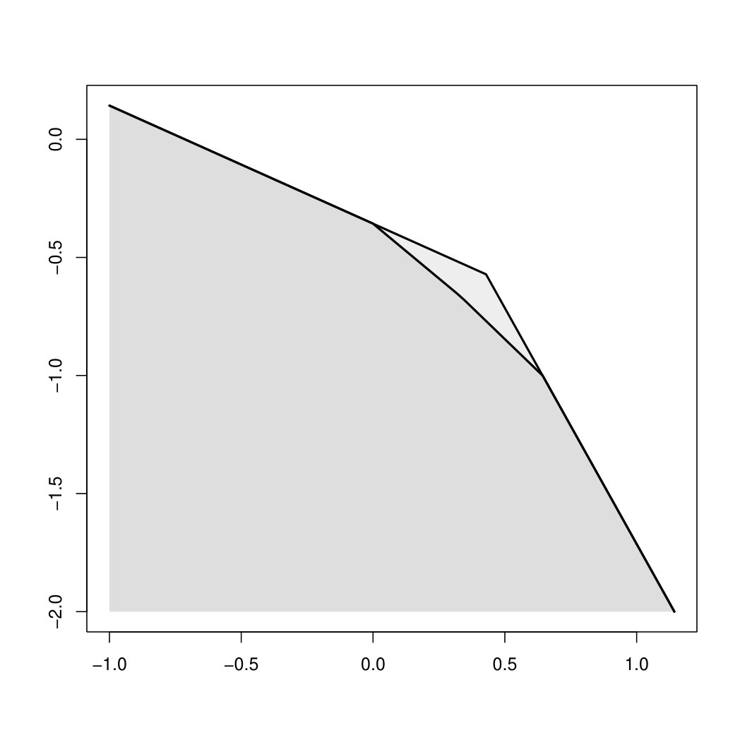 Figure 1
Peer Reviews
No public reviews on file for this paper yet. If you reviewed it on a platform where reviews are public (OpenReview, ICLR, NeurIPS, ICML), you can paste yours below so the community can read it here.
Videos
No videos yet. Explain this paper in a talk, walkthrough, or lecture? Add one.
Nonlinear expectations of random sets
Ilya Molchanov and Anja Mühlemann
University of Bern, Institute of Mathematical Statistics
and Actuarial Science, Alpeneggstrasse 22, CH-3012 Bern, Switzerland
Abstract
Sublinear functionals of random variables are known as sublinear expectations; they are convex homogeneous functionals on infinite-dimensional linear spaces. We extend this concept for set-valued functionals defined on measurable set-valued functions (which form a nonlinear space), equivalently, on random closed sets. This calls for a separate study of sublinear and superlinear expectations, since a change of sign does not convert one to the other in the set-valued setting.
We identify the extremal expectations as those arising from the primal and dual representations of them. Several general construction methods for nonlinear expectations are presented and the corresponding duality representation results are obtained. On the application side, sublinear expectations are naturally related to depth trimming of multivariate samples, while superlinear ones can be used to assess utilities of multiasset portfolios.
1 Introduction
Fix a probability space . A sublinear expectation is a real-valued function defined on the space of -integrable random variables (with ), such that
[TABLE]
for each deterministic , the function is monotone,
[TABLE]
homogeneous
[TABLE]
and subadditive
[TABLE]
see [24], who brought sublinear expectations to the realm of probability theory and established their close relationship to solutions of backward stochastic differential equations. A superlinear expectation satisfies the same properties with (1.2) replaced by
[TABLE]
In many studies, the homogeneity property together with the sub- (super-) additivity is replaced by the convexity of and the concavity of . These nonlinear expectations may be defined on a larger family than or on its subfamily; it is necessary to assume that the domain of definition contains all constants and is closed under addition and multiplication by positive constants. The range of values may be extended to for the sublinear expectation and to for the superlinear one.
The choice of notation and is explained by the fact that the superlinear expectation can be viewed as a utility function that allocates a higher utility value to the sum of two random variables in comparison with the sum of their individual utilities, see [5]. If random variable models a financial gain, then is called a coherent risk measure. Property (1.1) is then termed cash invariance, and the superadditivity property is turned into subadditivity due to the change of sign. The subadditivity of risk means that the sum of two random variables bears at most the same risk as the sum of their risks; this is justified by the economic principle of diversification.
It is easy to see that is a sublinear expectation if and only if
[TABLE]
is a superlinear one, and in this case and are said to form an exact dual pair. The sublinearity property yields that
[TABLE]
so that . The interval generated by an exact dual pair of nonlinear expectations characterises the uncertainty in the determination of the expectation of . In finance, such intervals determine price ranges in illiquid markets, see [19].
We equip the space with the -topology based on the standard pairing of and with . It is usually assumed that is lower semicontinuous and is upper semicontinuous in the -topology. Given that and take finite values, general results of functional analysis concerning convex functions on linear spaces imply the semicontinuity property if (see [15]); it is additionally imposed if . A nonlinear expectation is said to be law invariant (more exactly, law-determined) if it takes the same value on identically distributed random variables, see [8, Sec. 4.5].
A rich source of sublinear expectations is provided by suprema of conventional (linear) expectations taken with respect to several probability measures. Assuming the -lower semicontinuity, the bipolar theorem yields that this is the only possible case, see [5] and [15]. Then
[TABLE]
is the supremum of expectations over a convex -closed cone in ; the superlinear expectation is obtained by replacing the supremum with the infimum. In the following, we assume that (1.5) holds and the representing set is chosen in such a way to ensure that the corresponding sublinear and superlinear expectations are law invariant, that is, with each , contains all random variables identically distributed as .
A random closed set in Euclidean space is a random element with values in the family of closed sets in such that is a measurable event for all compact sets in , see [20]. In other words, a random closed set is a measurable set-valued function. A random closed set is said to be convex if almost surely belongs to the family of closed convex sets in . For convex random sets in Euclidean space, the measurability condition is equivalent to the fact that the support function of (see (2.2)) is a random function on with values in .
In the set-valued setting, it is natural to replace the inequalities (1.2) and (1.3) with the inclusions. For sets, the minus sign corresponds to the reflection with respect to the origin; it does not alter the direction of the inclusion, and so there is no direct link between set-valued sublinear and superlinear expectations. Set inclusions are always considered nonstrict, e.g., allows for .
This paper aims to systematically explore nonlinear set-valued expectations. Section 2 recalls the classical concept of the (linear) selection expectation for random closed sets, see [2] and [20, Sec. 2.1]. A random vector is said to be a selection of if almost surely. The selection expectation is defined as the closure of the set of expectations of all integrable selections of (the primal representation) or by considering the expected support function (being the dual representation). In this section, we introduce a suitable convergence concept for (possibly, unbounded) random convex sets based on linear functionals applied to the support function.
Nonlinear expectations of random convex sets are introduced in Section 3. The definitions refine the properties of nonlinear expectations stated in [20, Sec. 2.2.7]. Basic examples of such expectations and more involved constructions are considered with a particular attention to the expectations of random singletons and half-spaces. It is also explained how the set-valued expectation applies to random convex functions and how it is possible to get rid of the homogeneity property and to extend the setting to convex/concave functionals.
Among the rather vast variety of nonlinear expectations, it is possible to identify extremal ones: the minimal sublinear expectation of is the convex hull of nonlinear expectations of all sets from some family that yields as their union. In the case of selections, this becomes a direct generalisation of the primal representation for the selection expectation. The maximal superlinear extension is the intersection of nonlinear expectations of all half-spaces containing the random set. While in the linear case the both coincide and provide two equivalent definitions of the selection expectation, in general, the two constructions differ.
Nonlinear maps restricted to the family of -integrable random vectors have been studied in [4, 9], the comprehensive duality results can be found in [7]. In our framework, these studies concern the cases when the argument of a superlinear expectation is the sum of a random vector and a convex cone. However, for general set-valued arguments, it is not possible to rely the approach of [9, 7], since the known techniques of set-valued optimisation theory (see, e.g., [16]) are not applicable.
The key technique suitable to handle nonlinear expectations relies on the bipolar theorem. A direct generalisation of this theorem for functional of random convex sets is not feasible, since random convex sets do not form a linear space. Section 5 provides duality results for sublinear expectations and Section 6 for the superlinear ones. Specifically, the constant preserving minimal sublinear expectations are identified. For the superlinear expectation, the family of random closed convex sets such that the sublinear expectation contains the origin is a convex cone. However, it is rather tricky to use the separation results, since linear functions (such as the selection expectation) may have trivial values on unbounded integrable random sets. For instance, the selection expectation of a random half-space with a nondeterministic normal is the whole space; in this case the superlinear expectation is not dominated by any nontrivial linear one. In order to handle such situations, the duality results for superlinear expectations are proved for the maximal superlinear expectation. It is shown that the superlinear expectation of a singleton is usually empty; in order to come up with a nontrivial minimal extension, singletons in the definition of the minimal extension are replaced by translated cones.
Some applications are outlined in Section 7. Sublinear expectations are useful as depth functions in order to identify outliers in samples of random sets. Such samples often appear in partial identified models in econometrics, see [22]. The superlinear expectation is closely related to measuring multivariate risk in finance and to multivariate utilities. Superlinear expectations are useful to describe the utility, since the utility of the sum of two portfolios described by random sets “dominates” the sum of their individual utilities. We show that the minimal extension of a superlinear expectation is closely related to the selection risk measure of lower random sets considered in [21].
Appendix presents a self-contained proof of the fact that vector-valued sublinear expectations of random vectors necessarily split into sublinear expectations applied to each component of the vector. This fact reiterates the point that the set-valued setting is essential for defining nonlinear expectations of random vectors.
Note the following notational conventions: denote random closed convex sets, is a deterministic closed convex set, and are -integrable random vectors and random variables, and are -integrable vectors and variables with , is usually a random vector from the unit sphere , and are deterministic points from .
2 Selection expectation
2.1 Integrable random sets and selection expectation
Let be a random closed set in , which is always assumed to be almost surely non-empty. A random vector is called a selection of if almost surely. Let denote the family of -integrable selections of for , essentially bounded ones if , and all selections if . If is not empty, then is called -integrable, shortly integrable if . This is the case if is -integrably bounded, that is, is -integrable (essentially bounded if ).
If is integrable, then its selection expectation is defined by
[TABLE]
which is the closure of the set of expectations of all integrable selections of , see [20, Sec. 2.1.2]. If is integrably bounded, then the closure on the right-hand side is not needed, is compact, and also almost surely convex if is convex or the underlying probability space is non-atomic. From now on, we assume that all random closed sets are almost surely convex.
The support function of a non-empty set in is defined by
[TABLE]
allowing for possibly infinite values if is not bounded, where denotes the scalar product. Due to homogeneity, the support function is determined by its values on the unit sphere .
If is an integrable random closed set, then its expected support function is the support function of , that is,
[TABLE]
see [20, Th. 2.1.38]. Thus,
[TABLE]
which may be seen as the dual representation of the selection expectation with (2.1) being its primal representation. [1] provide an axiomatic Daniell–Stone type characterisation of the selection expectation. Property (2.3) can be also expressed as
[TABLE]
meaning that in this case it is possible to interchange the expectation and the supremum. If is an integrable random closed set and is a sub--algebra of , the conditional expectation is identified by its support function, being the conditional expectation of the support function of , see [12] and [20, Sec. 2.1.6].
The dilation (scaling) of a closed set is defined as for . For two closed sets and , their closed Minkowski sum is defined by
[TABLE]
and the sum is empty if at least one summand is empty. If at least one of and is compact, then the closure on the right-hand side is not needed. We write shortly instead of for .
If and are random closed convex sets, then is a random closed set, see [20, Th. 1.3.25]. The selection expectation is linear on integrable random closed sets, that is,
[TABLE]
see, e.g., [20, Prop. 2.1.32].
Let be a deterministic closed convex cone in which is distinct from the whole space. If , then is said to be -closed. Due to the closed Minkowski sum on the right-hand side, is also topologically closed. Let denote the family of all -closed convex sets in (including the empty set), and let be the family of all -integrable random sets with values in . Any random set from is necessarily a.s. non-empty. By
[TABLE]
we denote the polar cone to .
Example 2.1*.*
If , then is the family of all convex closed sets in . If , then is the family of lower convex closed sets, and a random closed convex set with realisations in this family is called a random lower set.
Example 2.2*.*
Let be a convex closed cone in which does not coincide with the whole space. If for , then belongs to the space . For each , we have .
2.2 Support function at random directions
Let
[TABLE]
denote a half-space in , and let . Particular difficulties when dealing with unbounded random closed sets are caused by the fact that the support function of any deterministic argument may be infinite with probability one.
Example 2.3*.*
Let be the random half-space with the normal vector having a non-atomic distribution. Then is the whole space. The support function of is finite only on the random ray .
It is shown in [17, Cor. 3.5] that each random closed convex set satisfies
[TABLE]
where
[TABLE]
is the smallest half-space with outer normal that contains . If is a.s. -closed, (2.6) holds with running through the family of selections of .
For each , the support function is a random variable with values in , see [17, Lemma 3.1]. While is not necessarily integrable, its negative part is always integrable if is -integrable. Indeed, choose any , and write
[TABLE]
The second summand on the right-hand side is integrable, while the first one is nonnegative.
Lemma 2.4**.**
Let . If for all , then a.s.
Proof.
For each measurable event , replacing with yields that
[TABLE]
whence a.s. The same holds for a general by splitting it into the cases when and . For a general , we have a.s. with , . Thus, a.s. for all , and the statement follows from [17, Cor. 3.6]. ∎
Corollary 2.5**.**
The distribution of is uniquely determined by for .
Proof.
Apply Lemma 2.4 to , so that the values of identify all -integrable selections of , and note that equals the closure of the family of its -integrable selections, see [20, Prop. 2.1.4]. ∎
A random closed set is called Hausdorff approximable if it appears as the almost sure limit in the Hausdorff metric of random closed sets with at most a finite number of values. It is known [20, Th. 1.3.18] that all random compact sets are Hausdorff approximable, as well as those that appear as the sum of a random compact set and a random closed set with at most a finite number of possible values. The random closed set from Example 2.3 is not Hausdorff approximable.
The distribution of a Hausdorff approximable -integrable random closed convex set is uniquely determined by the selection expectations for all , actually it suffices to let be all measurable indicators, see [11] and [20, Prop. 2.1.33]. If is Hausdorff approximable, then its selections are identified by the condition for all events . By passing to the support functions, we arrive at a variant of Lemma 2.4 with for all and .
2.3 Convergence of random closed convex sets
Convergence of random closed sets is typically considered in probability, almost surely, or in distribution. In the following we need to define -type convergence concepts suitable to deal with unbounded random convex sets.
The space is equipped with the -topology, that is, means that for all .
Lemma 2.6**.**
*If is a -integrable random -closed convex set, then is a non-empty convex -closed and -closed subset of . *
Proof.
If and in , then
[TABLE]
for all . Thus, is a selection of by Lemma 2.4. The statement concerning -closedness is obvious. ∎
A sequence , , is said to converge to scalarly in (shortly, scalarly) if for all , where the convergence is understood in the extended line . Since equals the support function of in direction , this convergence is the scalar convergence as convex sets in , see [26].
3 General nonlinear set-valued expectations
3.1 Definitions
Fix and a convex closed cone distinct from the whole space.
Definition 3.1**.**
A sublinear set-valued expectation is a function such that:
- i)
for each deterministic ,
[TABLE]
(additivity on deterministic singletons); 2. ii)
for all deterministic ; 3. iii)
if almost surely (monotonicity); 4. iv)
for all (homogeneity); 5. v)
is subadditive, that is,
[TABLE]
for all -integrable random closed convex sets and .
A superlinear set-valued expectation satisfies the same properties with the exception of ii) replaced by and (3.2) replaced by the superadditivity property
[TABLE]
The nonlinear expectations and are said to be law invariant, if they retain their values on identically distributed random closed convex sets.
Proposition 3.2**.**
Nonlinear expectations on take values from .
Proof.
If , then a.s., whence . Therefore, . ∎
While the argument of nonlinear expectations is a.s. non-empty, may be empty and then the right-hand side of (3.3) is also empty. However, if is empty for some , then for , hence
[TABLE]
is empty for all -integrable random sets . In view of this, it is assumed that sublinear expectations take non-empty values. We always exclude the trivial cases, when or for all .
The homogeneity property immediately implies that and are cones if is almost surely a cone, that is, a.s. for all . Therefore, it is only possible to conclude that is a closed convex cone, which may be strictly larger than . By Proposition 3.2, is either or is empty.
The sublinear (respectively, superlinear) expectation is said to be normalised if (respectively, ). We always have by property ii), and also , since for all , and is not identically empty.
The properties of the nonlinear expectations do not imply that they preserve deterministic convex closed sets. The family of invariant sets is closed under translations, dilations by positive reals, and for Minkowski sums, since if and , then
[TABLE]
A nonlinear expectation is said to be constant preserving if all non-empty deterministic sets from are invariant.
The superlinear and sublinear expectations form a dual pair if for each -integrable random closed convex set . In difference to the univariate setting, the exact duality relation (1.4) is useless; if , then is also a sublinear expectation, where is the reflection of with respect to the origin.
For a sequence of closed sets, its lower limit, , is the set of limits for all convergent sequences , , and its upper limit, , is the set of limits for all convergent subsequences , .
The sublinear expectation is called lower semicontinuous if
[TABLE]
and is upper semicontinuous if
[TABLE]
for a sequence of random closed convex sets converging to in the chosen topology, e.g. scalarly lower semicontinuous if scalarly converges to . Note that the lower semicontinuity definition is weaker than its standard variant for set-valued functions that would require that is a subset of , see [14, Prop. 2.35].
Remark 3.3*.*
It is possible to consider nonlinear expectations defined only on some special random sets, e.g., singletons or half-spaces. It is only required that the family of such sets is closed under translations, dilations by positive reals, and for Minkowski sums.
The family is often ordered by the reverse inclusion ordering; then the terminology is correspondingly adjusted, e.g., the superlinear expectation becomes sublinear. However, we systematically consider the conventional inclusion order.
Remark 3.4*.*
Motivated by financial applications, it is possible to replace the homogeneity and sub- (super-) additivity properties with convexity or concavity, e.g.,
[TABLE]
However, then can be turned into a superlinear expectation for random sets in the space by letting
[TABLE]
The arguments of are random closed convex sets ; they form a family closed for dilations, Minkowski sums and translations by singletons from . Note that selections of are given by with being a selection of . In view of this, all results in the homogeneous case apply to the convex case if dimension is increased by one.
3.2 Examples
The simplest example is provided by the selection expectation, which is linear and law invariant on all integrable random convex sets.
Example 3.5* (Fixed points and support).*
Let
[TABLE]
denote the set of fixed points of a random closed set . If is almost surely convex, then is also almost surely convex, and if is compact with a positive probability, then is compact. It is easy to see that , whence is a law invariant superlinear expectation. With a similar idea, it is possible to define the sublinear expectation as the support of , which is the set of points such that hits any open neighbourhood of with a positive probability. By the monotonicity property, for any , whence is a subset of any other normalised superlinear expectation of . By a similar argument, dominates any other constant preserving sublinear expectation.
Example 3.6* (Half-lines).*
Fix and let . Then is superlinear if and only if is sublinear in the usual sense of (1.2). For random sets of the type , the superlinearity of corresponds to the univariate superlinearity of . Therefore, the nature of a set-valued nonlinear expectation depends not only on the background numerical one, but also on the construction of relevant random sets. The situation becomes more complicated in higher dimensions, where complements of convex sets are not necessarily convex and the Minkowski sum of complements is not equal to the complement of the sum.
Example 3.7* (Random intervals).*
Let be a random interval on the line with , and let . Then is the interval formed by a numerical superlinear expectation of and a numerical sublinear expectation of such that for all , e.g., if and are an exact dual pair. The superlinear expectation may be empty.
3.3 Expectations of singletons and half-spaces
The additivity property on deterministic singletons immediately yields the following useful fact.
Lemma 3.8**.**
We have , and the same holds for the superlinear expectation.
Fix . Restricted to singletons, the sublinear expectation is a homogeneous map that satisfies
[TABLE]
Note that is not necessarily a singleton. If is a singleton for each , then is linear on . Assuming its lower semicontinuity, it becomes the usual (linear) expectation. The following result concerns the superlinear expectation of singletons. For a general cone , a similar result holds with singletons replaced by sets .
Proposition 3.9**.**
Let . For each and any normalised superlinear expectation , the set is either empty or a singleton, and is additive on the family of all singletons with non-empty .
Proof.
By (3.3) applied to and , we have
[TABLE]
whence is either empty or is a singleton, and then . If and are singletons (and so are non-empty) for , then
[TABLE]
whence the inclusion turns into the equality. ∎
In view of Proposition 3.9 and imposing the upper semicontinuity property on the superlinear expectation, equals or is empty for each -integrable . The family of such that is a convex cone in .
Proposition 3.10**.**
If a.s. for being an independent copy of , then for each law invariant sublinear expectation .
Proof.
By subadditivity and law invariance,
[TABLE]
Proposition 3.10 applies if is a half-space with a non-atomic , so that each law invariant sublinear expectation on such random sets takes trivial values.
Example 3.11*.*
Let . If for a vector-valued function , then splits into the vector of superlinear expectations applied to the components of , see Theorem A.1.
3.4 Nonlinear expectations of random convex functions
A lower semicontinuous convex function yields a convex set in such that
[TABLE]
The obtained support function is called the perspective transform of , see [13]. Note that can be recovered by letting in the support function of .
If , , is a random nonnegative lower semicontinuous convex function, then its sublinear expectation can be defined as , and the superlinear one is defined similarly. With this definition, all constructions from this paper apply to random functions.
4 Extensions of nonlinear expectations
4.1 Minimal extension
The minimal extension of a sublinear set-valued expectation on random sets from is defined by
[TABLE]
where denotes the closed convex hull operation. It extends a sublinear expectation defined on sets to all -integrable random closed sets such that a.s. In terms of support functions, the minimal extension is given by
[TABLE]
Proposition 4.1**.**
If is a sublinear expectation defined on random sets for , then its minimal extension (4.1) is a sublinear expectation.
Proof.
The additivity of on deterministic singletons follows from this property of . For a deterministic ,
[TABLE]
The homogeneity and monotonicity properties of are obvious. The subadditivity follows from the fact that is the -closure of the sum , see [20, Prop. 2.1.6]. ∎
4.2 Maximal extension
Extending a superlinear expectation from its values on half-spaces yields its maximal extension
[TABLE]
being the intersection of superlinear expectations of random half-spaces almost surely containing . Recall that .
Proposition 4.2**.**
If is superlinear on half-spaces with the same normal, that is,
[TABLE]
for and , and is scalarly upper semicontinuous on half-spaces with the same normal, that is,
[TABLE]
if in , then its maximal extension given by (4.3) is superlinear and upper semicontinuous with respect to the scalar convergence of random closed convex sets. If is law invariant on half-spaces, then is law invariant.
Proof.
The additivity on deterministic singletons follows from the fact that for all . If is deterministic, then
[TABLE]
The homogeneity and monotonicity properties of the extension are obvious. For two -integrable random closed convex sets and , (4.4) yields that
[TABLE]
Assume that scalarly converges to . Let and for some . Then for all . Since in , upper semicontinuity on half-spaces yields that , whence for all . Therefore, , confirming the upper semicontinuity of the maximal extension. The law invariance property is straightforward. ∎
It is possible to let in (4.3) be deterministic and define
[TABLE]
With this reduced maximal extension, the superlinear expectation is extended from its values on half-spaces with deterministic normal vectors. Note that the reduced maximal extension may be equal to the whole space, e.g., for being a half-space with a nondeterministic normal. It is obvious that and is constant preserving. The reduced maximal extension is particularly useful for Hausdorff approximable random closed sets.
4.3 Exact nonlinear expectations
It is possible to apply the maximal extension to the sublinear expectation and the minimal extension to the superlinear one, resulting in and . The monotonicity property yields that, for each -integrable random closed set ,
[TABLE]
It is easy to see that each extension is an idempotent operation, e.g., the minimal extension of coincides with .
A nonlinear sublinear expectation is said to be minimal (respectively, maximal) if it coincides with its minimal (respectively, maximal) extension. The superlinear expectation is said to be reduced maximal if coincides with . Since random convex closed sets can be represented either as families of their selections or as intersections of half-spaces, the minimal representation may be considered a primal representation of an exact nonlinear expectation, while the maximal representation becomes the dual one.
If (4.6) holds with the equalities, then is said to be exact. The same applies to superlinear expectations. Note that the selection expectation is exact on all integrable random closed convex sets, its minimality corresponds to (2.1) and maximality becomes (2.3).
5 Sublinear set-valued expectations
5.1 Duality for minimal sublinear expectations
The minimal sublinear expectation is determined by its restriction on random sets ; the following result characterises such a restriction.
Lemma 5.1**.**
A map for is a -lower semicontinuous normalised sublinear expectation if and only if for , and
[TABLE]
where , , are convex -closed cones in , such that for all , for all , , and
[TABLE]
Proof.
Sufficiency. For linearly independent and , each satisfies with and . Thus, only if . Therefore,
[TABLE]
Since for any ,
[TABLE]
whence the function is sublinear in and so is a support function.
The additivity property on singletons follows from the construction, since
[TABLE]
for each deterministic . Furthermore, , whence . The homogeneity property is obvious. The function is subadditive, since
[TABLE]
For , the set is closed in . Indeed, if , then in let be one the basis vectors to confirm that . Since is the support function of the closed set in direction , it is lower semicontinuous as function of , so that (3.4) holds.
Necessity. By Proposition 3.2, the support function is infinite for . For , let be the set of such that . The map is a sublinear map from to . By sublinearity, is a convex cone in , and for all . Furthermore, is closed with respect to the scalar convergence by the assumed lower semicontinuity of . Hence, it is closed with respect to the convergence in .
Note that , and let
[TABLE]
be the polar cone to . For , we have and . Consider . Letting for an event and deterministic with , we obtain a member of , whence each satisfies whenever . Thus, a.s., and letting yields that for some and all . The subadditivity property of the support function of yields that for . By a Banach space analogue of [25, Th. 1.6.9], the polar to is the closed sum of the polars, whence (5.2) holds.
By the definition of ,
[TABLE]
Since is convex and -closed, the bipolar theorem yields that
[TABLE]
Theorem 5.2**.**
A function on -integrable random closed convex sets is a scalarly lower semicontinuous minimal normalised sublinear expectation if and only if admits the representation
[TABLE]
and for , where satisfy the conditions of Lemma 5.1.
Proof.
Necessity. Lemma 5.1 applies to the restriction of onto random sets . By the minimality assumption, coincides with its minimal extension (4.2). By Lemma 5.1, for ,
[TABLE]
where (2.4) has been used.
Sufficiency. The right-hand side of (5.3) is sublinear in and so is a support function. The additivity on singletons, monotonicity, subadditivity and homogeneity properties of are obvious. For a deterministic , the sublinearity of the support function yields that
[TABLE]
whence .
The minimality of follows from
[TABLE]
Since the support function of given by (5.3) is the supremum of scalarly continuous functions of , the minimal sublinear expectation is scalarly lower semicontinuous. ∎
Corollary 5.3**.**
If for all , then for all -integrable and any scalarly lower semicontinuous normalised minimal sublinear expectation .
Proof.
By (5.3), for all . ∎
Remark 5.4*.*
The sublinear expectation given by (5.3) is law invariant if and only if the sets are law-complete, that is, with each , the set contains all random vectors that share distribution with .
Example 5.5*.*
Let be a random matrix with being the identity matrix, and let , . Then (5.3) turns into , whence . It is possible to let belong to a family of such matrices; then is the closed convex hull of the union of for all such . In this example, is not solely determined by . This sublinear expectation is not necessarily constant preserving.
Example 5.6* (Random half-space).*
Let with and . By (5.3), is finite for only if each with satisfies a.s. with . Then
[TABLE]
If the normal is deterministic and
[TABLE]
then with
[TABLE]
Otherwise, .
5.2 Exact sublinear expectation
Consider now the situation when, for each , the value of is solely determined by the distribution of . This is the case if the supremum in (5.3) involves only such that for some . The following result shows that this condition characterises constant preserving minimal sublinear expectations, which then necessarily become exact ones.
Theorem 5.7**.**
A function on -integrable random closed convex sets from is a scalarly lower semicontinuous constant preserving minimal sublinear expectation if and only if for , and
[TABLE]
where , , are convex -closed cones in , such that for all , and for all .
Proof.
Sufficiency. If , , satisfy the imposed conditions, then , , satisfy the conditions of Lemma 5.1. Indeed, for all , and
[TABLE]
for all . If is deterministic, then
[TABLE]
whence is constant preserving.
Necessity. Since is minimal, the support function of is given by (5.3). The constant preserving property yields that for all half-spaces with . By the argument from Example 5.6, the minimal sublinear expectation of a half-space is distinct from the whole space only if (5.4) holds.
The properties of imply the imposed properties of . Indeed, assume that , so that . Hence, , meaning that is the norm limit of for and , . The linear independence of and yields that and , whence . ∎
It is possible to rephrase (5.5) as
[TABLE]
for numerical sublinear expectations
[TABLE]
defined by an analogue of (1.5). Since the negative part of is -integrable, it is possible to consistently let in (5.7) if is not -integrable.
Corollary 5.8**.**
Each scalarly lower semicontinuous constant preserving minimal sublinear expectation is exact.
Proof.
Since (5.5) yields that if is random, the maximal extension of by an analogue of (4.3) reduces to deterministic and so is the reduced maximal extension. For and , we have , cf. Example 5.6. Thus, the reduced maximal extension of is given by
[TABLE]
Comparing with (5.6), we see that . The opposite inclusion is obvious, whence . ∎
Corollary 5.9**.**
If is a scalarly lower semicontinuous constant preserving minimal normalised sublinear expectation, then for each deterministic .
Corollary 5.10**.**
Assume that is scalarly lower semicontinuous constant preserving minimal law invariant sublinear expectation. Then for all and any sub--algebra of . In particular, .
Proof.
The law invariance of implies that is law invariant. The sublinear expectation is dilatation monotonic, meaning that for all , see [8, Cor. 4.59] for this fact derived for risk measures. The statement follows from (5.6). ∎
For a -integrable random closed convex set , its Firey -expectation is defined by . The next result follows from Hölder’s inequality applied to in (5.5).
Corollary 5.11**.**
If admits representation (5.5), then
[TABLE]
The following result identifies a particularly important case, when the families do not depend on . This property essentially means that the sublinear expectation preserves centred balls. By denote the ball of radius centred at the origin.
Theorem 5.12**.**
A scalarly lower semicontinuous constant preserving minimal superlinear expectation satisfies for all and (depending on ) if and only if (5.5) holds with for all . Then
[TABLE]
where admits the representation (1.5). Furthermore,
[TABLE]
Proof.
Assume that are constructed as in the proof of Theorem 5.7, so that is maximal for each . The right-hand side of
[TABLE]
does not depend on if and only if for all .
Representation (5.7) follows from (5.6) with . In view of (1.5),
[TABLE]
By (5.7), the support functions of the both sides of (5.8) are identical. ∎
If is a singleton, there is no need to take the convex hull on the right-hand side of (5.8).
Example 5.13*.*
For an integrable and , consider the sublinear expectation
[TABLE]
It is easy to see that is a minimal constant preserving sublinear expectation; it is given by (5.7) with the corresponding numerical sublinear expectation , being the expected maximum of i.i.d. copies of . By Corollary 5.8, this sublinear expectation is exact.
Example 5.14*.*
For , let be the family of random variables with values in and such that . Furthermore, let be the cone generated by , that is . In finance, the set generates the average Value-at-Risk, which is the risk measure obtained as the average quantile, see [8]. Similarly, the numerical sublinear and superlinear expectations generated by this set are represented as average quantiles. Namely, is the average of the quantiles of at levels , and is the average of the quantiles at levels . The corresponding set-valued sublinear expectation satisfies .
6 Superlinear set-valued expectations
6.1 Duality for maximal superlinear expectations
Consider a superlinear expectation defined on . If , we deal with all -integrable random closed convex sets. Recall that is the polar cone to .
Theorem 6.1**.**
A map is a scalarly upper semicontinuous normalised maximal superlinear expectation if and only if
[TABLE]
for a collection of convex -closed cones parametrised by and such that is strictly larger than for each deterministic .
Proof.
Necessity. Fix , and let be the set of such that contains the origin. Since , we have . Since , the family does not contain for and .
If in , then for all , whence scalarly in . Therefore,
[TABLE]
by the assumed upper semicontinuity of . Thus, is a convex -closed cone in . Consider its positive dual cone
[TABLE]
Since , we have whenever a.s. In view of this, if is a.s. nonnegative, then a.s. contains zero and so . Thus, each from is a.s. nonnegative. The bipolar theorem yields that
[TABLE]
Since , (6.2) yields that the cone is strictly larger than . Since is assumed to be maximal, (4.3) implies that
[TABLE]
Sufficiency. It is easy to check that given by (6.1) is additive on deterministic singletons, homogeneous and monotonic. If is deterministic, then letting in (6.1) be deterministic and using the nontriviality of yield that . Furthermore, , since contains the origin and so is not empty.
The superadditivity of follows from the fact that
[TABLE]
It is easy to see that coincides with its maximal extension.
Note that (6.1) is equivalently written as
[TABLE]
If scalarly converges to and for , , then converges to for all and . Thus, , whence , and the upper semicontinuity of follows. ∎
In difference to the sublinear case (see Theorem 5.2), the cones from Theorem 6.1 do not need to satisfy additional conditions like those imposed in Lemma 5.1.
Corollary 6.2**.**
If for all , then for all -integrable and any scalarly upper semicontinuous maximal normalised superlinear expectation .
Proof.
Restrict the intersection in (6.1) to deterministic and , so that the right-hand side of (6.1) becomes . ∎
Example 6.3*.*
Let be the half-space with normal and . If , the maximal superlinear expectation of is given by
[TABLE]
Assume that and let with being an almost surely positive random variable. We have
[TABLE]
where is the numerical superlinear expectation with the generating set . In particular, if a.s., then
[TABLE]
Therefore, , where and for the exact dual pair and of nonlinear expectations with the representing set .
6.2 Reduced maximal extension
The following result can be proved similarly to Theorem 6.1 for the reduced maximal extension from (4.5).
Theorem 6.4**.**
A map is a scalarly upper semicontinuous normalised reduced maximal superlinear expectation if and only if
[TABLE]
for a collection of nontrivial convex -closed cones , .
It is possible to take the intersection in (6.3) over all , since for . Representation (6.3) can be equivalently written as the intersection of the half-spaces , where
[TABLE]
is a superlinear univariate expectation of for each . The superlinear expectation (6.3) is law invariant if the families are law-complete for all .
Corollary 6.5**.**
Let be a scalarly upper semicontinuous law invariant normalised reduced maximal superlinear expectation, and let the probability space be non-atomic. Then is dilatation monotonic, meaning that
[TABLE]
for each sub--algebra and all . In particular, .
Proof.
Since is law-complete, given by (6.4) is a law invariant concave function of . Thus, is dilatation monotonic by [8, Cor. 4.59], meaning that . Hence,
[TABLE]
Example 6.6*.*
If in (6.3) is nontrivial and does not depend on , then (6.3) turns into
[TABLE]
where given by (6.4) is the numerical superlinear expectation with the representing set . In this case, is the largest convex set whose support function is dominated by , that is,
[TABLE]
Note that may fail to be a support function. Since
[TABLE]
for , this reduced maximal superlinear expectation admits the equivalent representation as
[TABLE]
Example 6.7*.*
Let for a and a deterministic convex closed cone that is different from the whole space. Then
[TABLE]
If for all , then and
[TABLE]
If is a Riesz cone, then for some , since an intersection of translations of is again a translation of , see [18, Th. 26.11].
Example 6.8*.*
Let for independent copies of , noticing that the expectation is empty if the intersection is empty with positive probability. This superlinear expectation is neither maximal, nor even a reduced maximal one. For instance,
[TABLE]
so that the reduced maximal extension is the largest convex set whose support function is dominated by , . However, the support function of is the expectation of the largest sublinear function dominated by , and so may be a strict subset of .
For instance, let for . Then
[TABLE]
where the minimum is applied coordinatewisely to independent copies of , while is the largest convex set whose support function is dominated by , . Obviously,
[TABLE]
with a possibly strict inequality.
6.3 Minimal extension of a superlinear expectation
In any nontrivial case, the superlinear expectation of a nondeterministic singleton is empty. Indeed, if , then (6.3) yields that
[TABLE]
which is not empty only if
[TABLE]
for all . In the setting of Example 6.6, is empty unless for all . The latter means that for the exact dual pair of real-valued nonlinear expectations. Equivalently, if for some . If this is the case for all , then the minimal extension of is the set of fixed points of , see Example 3.5. Thus, it is not feasible to come up with a nontrivial minimal extension of the superlinear expectation if .
A possible way to ensure non-emptiness of the minimal extension of is to apply it to random sets from with a cone having interior points, since then at least one of and is almost surely infinite for all . The minimal extension of is given by
[TABLE]
The following result, in particular, implies that the union on the right-hand side of (6.8) is a convex set, cf. (4.1).
Theorem 6.9**.**
The function given by (6.8) is a superlinear expectation. If in (6.8) is reduced maximal and satisfies the conditions of Corollary 6.5, then its minimal extension is law invariant and dilatation monotonic.
Proof.
Let and belong to the union on the right-hand side of (6.8) (without closure). Then and , and the superlinearity of yields that
[TABLE]
for each . Since is a selection of , the convexity of easily follows.
The additivity on deterministic singletons, monotonicity and homogeneity properties are evident from (6.8). If is deterministic, then
[TABLE]
For the superadditivity property, consider and from the nonclosed right-hand side of (6.8) for and , respectively. Then and for some and . Hence,
[TABLE]
Now assume that is reduced maximal. Let be the -algebra generated by . The convexity of implies that is a selection of for any . By the dilatation monotonicity property from Corollary 6.5, it is possible to replace in (6.8) with the family of -measurable -integrable selections of . These families coincide for two identically distributed sets, see [20, Prop. 1.4.5]. The dilatation monotonicity follows from Corollary 6.5. ∎
Below we establish the upper semicontinuity of the minimal extension.
Theorem 6.10**.**
Assume that , is upper semicontinuous, and that for all nontrivial . Then the minimal extension is scalarly upper semicontinuous.
Proof.
It suffices to omit the closure in (6.8) and consider such that and scalarly in . For each , there exists a such that .
Assume first that and . Then is relatively compact in . Without loss of generality, assume that . Then for all . Taking expectation, letting and using the convergence and yield that . By Lemma 2.4, is a selection of . By the upper semicontinuity of ,
[TABLE]
Hence, for some , so that .
Assume now that . Let . This sequence is bounded in the -norm, and so assume without loss of generality that in . Since
[TABLE]
the upper semicontinuity of yields that . For each , we have . Dividing by , taking expectation, and letting yield that . Thus, almost surely. Given that , this contradicts the fact that contains the origin.
Similar reasons apply if , splitting the cases when is essentially bounded and when the essential supremum of converges to infinity. ∎
The exact calculation of involves working with all -integrable selections of , which is a very rich family even in simple cases, like . Since
[TABLE]
the superlinear expectation yields a computationally tractable upper bound on .
Example 6.11*.*
Assume that for and a deterministic convex closed lower set . Assume that in (6.8) is reduced maximal and satisfies conditions of Corollary 6.5. Then
[TABLE]
where is the family of selections of which are measurable with respect to the -algebra generated by . Indeed, is a subset of by Corollary 6.5.
Note that the minimal extension is not necessarily a maximal superlinear expectation. The following result describes its maximal extension.
Theorem 6.12**.**
Assume that is defined by (6.8), where is a scalarly upper semicontinuous reduced maximal superlinear expectation with representation (6.6). Then for all and , and the reduced maximal extension of coincides with .
Proof.
By (6.3), . In view of (6.9), it suffices to show that each also belongs to . Let be the projection of onto the subspace orthogonal to . It suffices to show that . Noticing that , it is possible to assume that for .
Consider . Then
[TABLE]
Since , we deduce that .
Since and coincide on half-spaces, the reduced maximal extension of is
[TABLE]
In view of (6.9), if
[TABLE]
This surely holds for and also for being a half-space with a deterministic normal. In general, may be a strict subset of as the following example shows, so superlinear expectations are not exact even on rather simple random sets of the type .
Example 6.13*.*
Assume that and consider which equally takes two possible values: the origin and . Let , where is the cone containing and with points and on its boundary, such that .
Let be the family from Example 5.14 and let be the corresponding superlinear expectation with the representing set . For each , equals the average of the -quantiles of over . If and takes two values with equal probabilities, then is the smaller value of . Then , so that coincides with in this case, see Example 6.8.
Now assume that . If equally likely takes two values and , then , and
[TABLE]
for all from . Since is a Riesz cone, for some , see Example 6.7. For , the linear function is dominated by if and by otherwise. By an elementary calculation,
[TABLE]
In view of Example 6.11, it suffices to consider selections of measurable with respect to the -algebra generated by ; these selections take two values from the boundary of with equal probabilities. The minimal extension can be found by (6.10), letting equally likely take two values and on the boundary of . Then
[TABLE]
Figure 1 shows and for , , and . It shows that the minimal extension may be indeed a strict subset of the reduced maximal superlinear expectation.
7 Applications
7.1 Depth-trimmed regions and outliers
Consider a sublinear expectation restricted to the family of -integrable singletons, and let . The map satisfies the properties of depth-trimmed regions imposed in [3], which are those from [27] augmented by the monotonicity and subadditivity.
Therefore, the sublinear expectation provides a rather generic construction of a depth-trimmed region associated with a random vector . In statistical applications, points outside or its empirical variant are regarded as outliers. The subadditivity property (3.2) means that, if a point is not an outlier for the convolution of two samples, then there is a way to obtain this point as the sum of two non-outliers for the original samples.
Example 7.1* (Zonoid-trimmed regions).*
Fix . For , define
[TABLE]
where is an -quantile of (in case of non-uniqueness, the choice of a particular quantile does not matter because of integration). The risk measure is called the average value-at-risk. Denote by the corresponding minimal sublinear expectation constructed by (5.7), so that for all . The set is the zonoid-trimmed region of at level , see [3] and [23]. This set can be obtained as
[TABLE]
where consists of all random variables with values in and expectation , see Example 5.14. This setting is a special case of Theorem 5.12 with . The value of controls the size of the depth-trimmed region, yields a single point, being the expectation of . The subadditivity property of zonoid-trimmed regions was first noticed by [4].
Example 7.2* (Lift expectation).*
Let be an integrable random closed convex set. Consider the random set in given by the convex hull of the origin and . The selection expectation is called the lift expectation of , see [6]. If is a singleton, then is the lift zonoid of , see [23]. By definition of the selection expectation, is the closure of the set of , where runs through the family of random variables with values in . Equivalently, belongs to if and only if for from the family , see Example 7.1. Thus, the minimal extension of from Example 7.1 is
[TABLE]
7.2 Parametric families of nonlinear expectations
Consider a dual pair and of nonlinear expectations such that for all random closed sets . Then it is natural to regard observations of that do not lie between the superlinear and sublinear expectation as outliers. For each , it is possible to quantify its depth with respect to the distribution of using parametric families of nonlinear expectations constructed as follows.
Let be independent copies of a -integrable random closed convex set . For a sublinear expectation ,
[TABLE]
is also a sublinear expectation. The only slightly nontrivial property is the subadditivity, which follows from the fact that
[TABLE]
If is a.s. non-empty, then
[TABLE]
yields a superlinear expectation, noticing that
[TABLE]
It is possible to consistently let if is empty with positive probability.
Proposition 7.3**.**
Let be a geometric random variable such that, for some , , , which is independent of , being i.i.d. copies of . Then
[TABLE]
is a sublinear expectation and, if a.s. for all , then
[TABLE]
is a superlinear expectation depending on .
Example 7.4*.*
Choosing in (7.1) and (7.2) yields a family of nonlinear expectations depending on parameter, which are also easy to compute.
It is easily seen that increases and decreases as declines. Define the depth of as
[TABLE]
It is easy to see that , . Furthermore, declines to the set of fixed points of and increases to the support of as , see Example 3.5. Thus, all closed convex sets satisfying have a positive depth.
In order to handle the empirical variant of this concept based on a sample of independent observations of , consider a random closed set that with equal probabilities takes one of the values . Its distribution can be simulated by sampling one of these sets with possible repetitions. Then it is possible to use the nonlinear expectations of in order to assess the depth of any given convex set, including those from the sample.
7.3 Risk of a set-valued portfolio
For a random variable interpreted as a financial outcome or gain, the value (equivalently, ) is used in finance to assess the risk of . It may be tempting to extend this to the multivariate setting by assuming that the risk is a -dimensional function of a random vector , with the conventional properties extended coordinatewisely. However, in this case the nonlinear expectations (and so the risk) are marginalised, that is, the risk of splits into a vector of nonlinear expectations applied to the individual components of , see Theorem A.1.
Moreover, assessing the financial risk of a vector is impossible without taking into account exchange rules that can be applied to its components. If no exchanges are allowed and only consumption is possible, then one arrives at positions being selections of . On the contrary, if the components of are expressed in the same currency with unrestricted exchanges and disposal (consumption) of the assets, then each position from the half-space is reachable from . Working with the random set also eliminates possible non-uniqueness in the choice of with identical sums.
In view of this, it is natural to consider multivariate financial positions as lower random closed convex sets, equivalently, those from with . The random closed set is said to be acceptable if , and the risk of is defined as . The superadditivity property guarantees that if both and are acceptable, then is acceptable. This is the classical financial diversification advantage formulated in set-valued terms.
If and , the minimal extension (6.8) is called the lower set extension of . If is reduced maximal, (6.6) yields that
[TABLE]
where is defined by applying the same superlinear expectation with representing set to each component of . Then
[TABLE]
In other words, is the closure of the set of all points dominated coordinatewisely by the superlinear expectation of at least one selection of . In [21], the origin-reflected set was called the selection risk measure of .
For set-valued portfolios , arising as the sum of a singleton and a (possibly random) convex cone , the maximal superlinear expectation (in our terminology), considered a function of only and not of , was studied by [9] and [10]. The case of general set-valued arguments was pursued by [21]. For the purpose of risk assessment, one can use any superlinear expectation. However, the sensible choices are the maximal superlinear expectation in view of its closed form dual representation, and the lower set extension in view of its direct financial interpretation (through its primal representation), meaning the existence of a selection with all acceptable components. Given that the minimal superlinear expectation may be a strict subset of the maximal one (see Example 6.13), the acceptability of under a maximal superlinear expectation may be a weaker requirement than the acceptability under the lower set extension.
Appendix Marginalisation of vector-valued sublinear functions
It may be tempting to consider vector-valued functions , which are sublinear, that is, for all , if a.s., for all , and
[TABLE]
Such a function may be viewed as a restriction of a sublinear set-valued expectation onto the family of sets and letting be the coordinatewise supremum of .
The following result shows that vector-valued sublinear expectations marginalise, that is, they split into sublinear expectations applied to each component of the random vector.
Theorem A.1**.**
If is a -lower semicontinuous vector-valued sublinear expectation, then
[TABLE]
for a collection of numerical sublinear expectations .
Proof.
The set is a -closed convex cone in . The polar cone is the set of all -valued measures such that
[TABLE]
for all . It is easy to see that each has all nonnegative components. The bipolar theorem yields that
[TABLE]
Since is constant preserving,
[TABLE]
so that for all deterministic . Hence,
[TABLE]
where the infimum is taken coordinatewisely.
Consider the set for some . Let denote the family of all nontrivial such that vanish for all . Note that if , then , that is the projections of and on each of the component coincide. If , then
[TABLE]
Assume that two components of do not vanish, say and . Then
[TABLE]
Thus, this latter set does not influence the coordinatewise infimum in (A.1) comparing to the sets obtained by letting . The same argument applies to with more than two nonvanishing components. Thus, the intersection in (A.1) can be taken over , whence the result. ∎
A similar result holds for superlinear vector-valued expectations.
Acknowledgements
IM is grateful to Ignacio Cascos for discussions and a collaboration on related works. This work was motivated by the stay of IM at the Universidad Carlos III de Madrid in 2012 supported by the Santander Bank. IM was also supported in part by Swiss National Science Foundation grants 200021_153597 and IZ73Z0_152292.
The reference list from the paper itself. Each links out to its DOI / PubMed record.
- 1[1] Ç. Ararat and B. Rudloff. A characterization theorem for Aumann integrals. Set-Valued Var. Anal. , 23:305–318, 2015.
- 2[2] R. J. Aumann. Integrals of set-valued functions. J. Math. Anal. Appl. , 12:1–12, 1965.
- 3[3] I. Cascos. Data depth: multivariate statistics and geometry. In W. S. Kendall and I. Molchanov, editors, New Perspectives in Stochastic Geometry , pages 398–426. Oxford University Press, Oxford, 2010.
- 4[4] I. Cascos and I. Molchanov. Multivariate risks and depth-trimmed regions. Finance and Stochastics , 11:373–397, 2007.
- 5[5] F. Delbaen. Monetary Utility Functions . Osaka University Press, Osaka, 2012.
- 6[6] M.-A. Diaye, G. A. Koshevoy, and I. Molchanov. Lift expectations of random sets and their applications. Statist. Probab. Lett. , 145:110–117, 2018.
- 7[7] S. Drapeau, A. H. Hamel, and M. Kupper. Complete duality for quasiconvex and convex set-valued functions. Set-Valued Var. Anal. , 24:253–275, 2016.
- 8[8] H. Föllmer and A. Schied. Stochastic Finance. An Introduction in Discrete Time . De Gruyter, Berlin, 2 edition, 2004.