Helper and Equivalent Objectives: An Efficient Approach to Constrained Optimisation
Tao Xu, Jun He, Changjing Shang

TL;DR
This paper introduces a novel multi-objective optimization approach using helper and equivalent objectives for constrained problems, demonstrating improved efficiency and performance over existing algorithms, especially on challenging wide gap problems.
Contribution
It proposes a new method that transforms constrained optimization into a multi-objective problem with helper and equivalent objectives, and provides theoretical and empirical validation of its effectiveness.
Findings
Shortens the crossing time of wide gap problems.
Achieves top performance on IEEE CEC2017 benchmarks.
Theoretically reduces exponential crossing time in hard problems.
Abstract
Numerous multi-objective evolutionary algorithms have been designed for constrained optimisation over past two decades. The idea behind these algorithms is to transform constrained optimisation problems into multi-objective optimisation problems without any constraint, and then solve them. In this paper, we propose a new multi-objective method for constrained optimisation, which works by converting a constrained optimisation problem into a problem with helper and equivalent objectives. An equivalent objective means that its optimal solution set is the same as that to the constrained problem but a helper objective does not. Then this multi-objective optimisation problem is decomposed into a group of sub-problems using the weighted sum approach. Weights are dynamically adjusted so that each subproblem eventually tends to a problem with an equivalent objective. We theoretically analyse the…
Click any figure to enlarge with its caption.
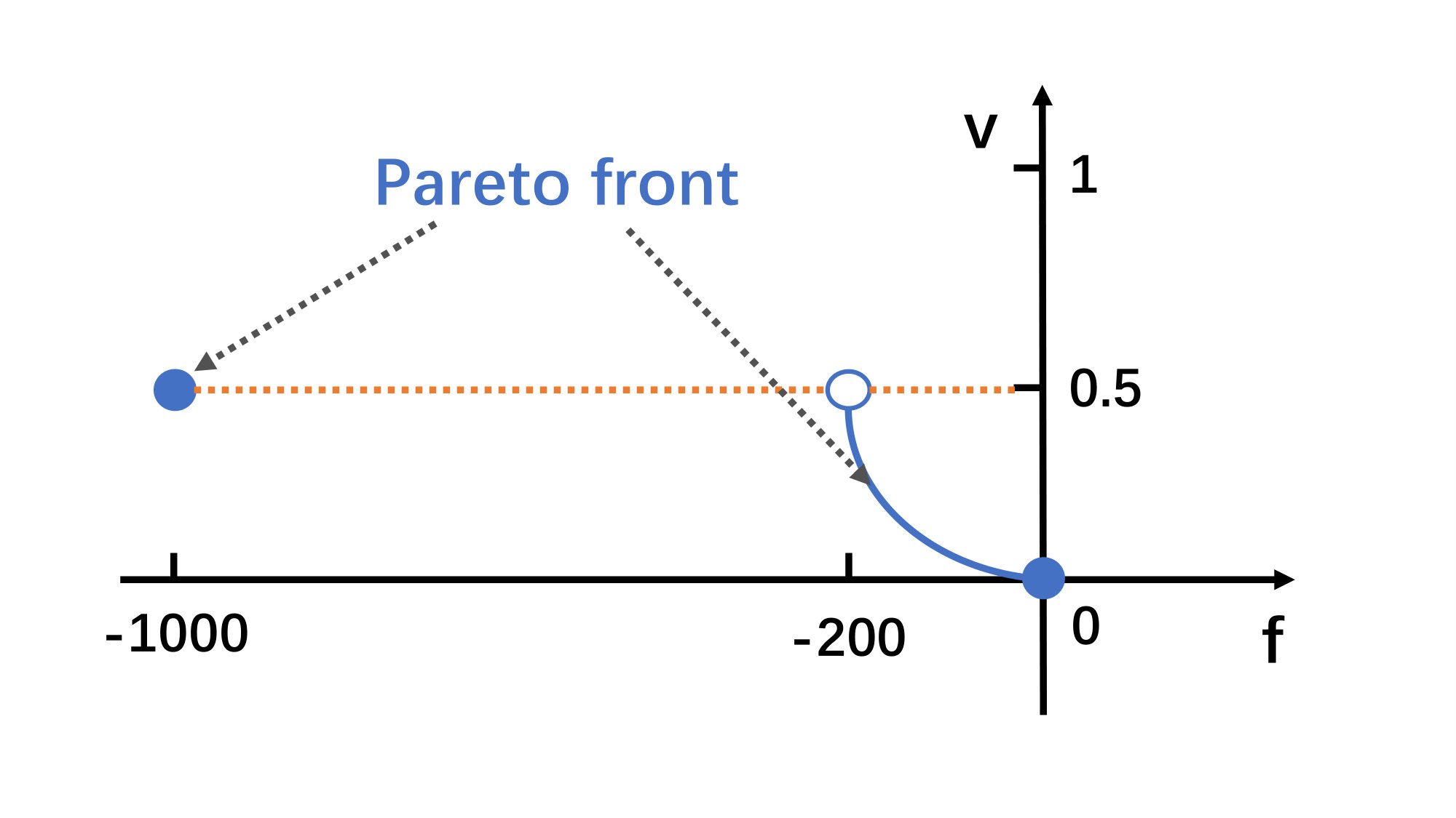 Figure 1
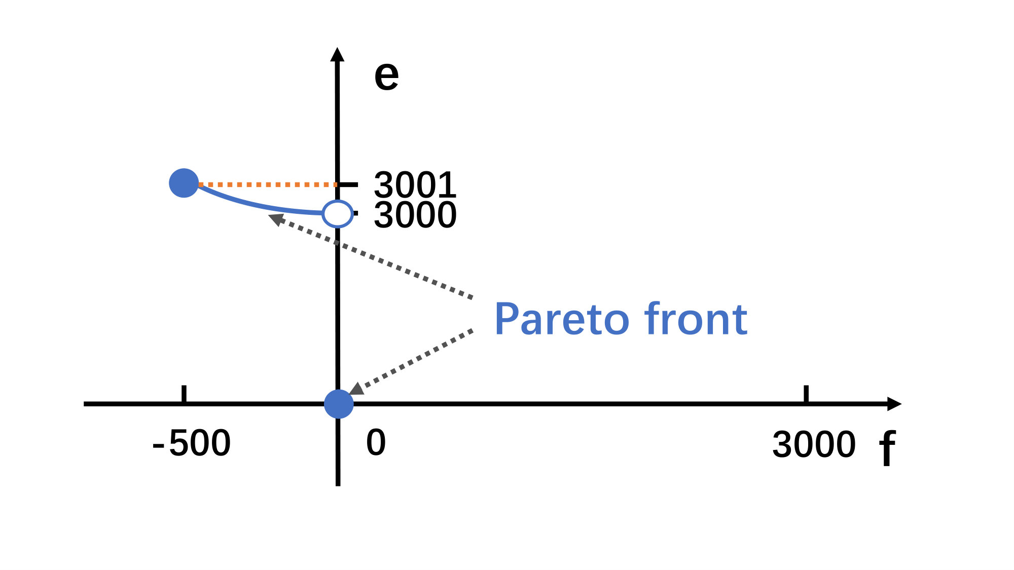 Figure 2
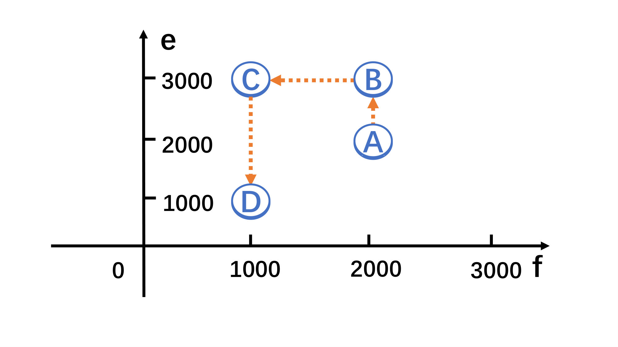 Figure 3
 Figure 4
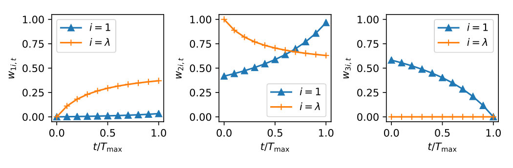 Figure 5
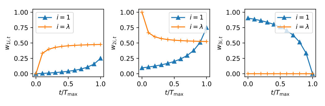 Figure 6
 Figure 7
| historical memory size | |
|---|---|
| number of strategies | |
| constant in strategy adaption | |
| threshold in strategy adaption | |
| the maximum size of archive | |
| tolerance for equivalent constraints |
| CEC2006 | |
|---|---|
| from CEC2006 benchmarks | |
| required population sizes | , |
| population size of | |
| constraint violation bias | |
| CEC2017 | |
| from CEC2017 benchmarks | |
| required population sizes | , |
| population size of | |
| constraint violation bias | |
| Algorithm/Dimension | Total | ||||
|---|---|---|---|---|---|
| CAL_LSAHDE(2017) | 421 | 420 | 469 | 478 | 1788 |
| LSHADE44+IDE(2017) | 310 | 394 | 422 | 392 | 1518 |
| LSAHDE44(2017) | 332 | 344 | 342 | 342 | 1360 |
| UDE(2017) | 341 | 372 | 377 | 438 | 1528 |
| MA_ES(2018) | 271 | 261 | 273 | 282 | 1087 |
| IUDE(2018) | 198 | 261 | 269 | 327 | 1055 |
| LSAHDE_IEpsilon(2018) | 222 | 278 | 324 | 372 | 1196 |
| DeCODE(2018) | 239 | 297 | 302 | 328 | 1166 |
| HCO-DE | 282 | 253 | 255 | 219 | 1009 |
| HECO-DE(FR) | 158 | 194 | 186 | 202 | 740 |
| HECO-DE | 154 | 139 | 156 | 205 | 654 |
| Algorithm/Dimension | Total | ||||
|---|---|---|---|---|---|
| CAL_LSAHDE(2017) | 507 | 508 | 569 | 582 | 2166 |
| LSHADE44+IDE(2017) | 381 | 486 | 524 | 483 | 1874 |
| LSAHDE44(2017) | 409 | 431 | 431 | 422 | 1693 |
| UDE(2017) | 431 | 479 | 480 | 537 | 1927 |
| MA_ES(2018) | 326 | 321 | 341 | 347 | 1335 |
| IUDE(2018) | 250 | 343 | 345 | 424 | 1362 |
| LSAHDE_IEpsilon(2018) | 277 | 354 | 420 | 472 | 1523 |
| DeCODE(2018) | 301 | 381 | 390 | 410 | 1482 |
| HECO-DE() | 172 | 199 | 218 | 261 | 850 |
| HECO-DE() | 194 | 149 | 181 | 242 | 766 |
| HECO-DE() | 177 | 174 | 197 | 241 | 789 |
| HECO-DE() | 195 | 192 | 204 | 210 | 801 |
| HECO-DE() | 189 | 208 | 200 | 222 | 819 |
| Algorithm/Dimension | Total | ||||
|---|---|---|---|---|---|
| CAL_LSAHDE(2017) | 508 | 511 | 572 | 583 | 2174 |
| LSHADE44+IDE(2017) | 373 | 485 | 518 | 482 | 1858 |
| LSAHDE44(2017) | 405 | 428 | 427 | 422 | 1682 |
| UDE(2017) | 423 | 471 | 465 | 532 | 1891 |
| MA_ES(2018) | 329 | 320 | 334 | 349 | 1332 |
| IUDE(2018) | 249 | 317 | 315 | 419 | 1300 |
| LSAHDE_IEpsilon(2018) | 276 | 341 | 415 | 475 | 1507 |
| DeCODE(2018) | 296 | 362 | 370 | 398 | 1426 |
| HECO-DE() | 254 | 207 | 243 | 287 | 991 |
| HECO-DE() | 186 | 177 | 186 | 234 | 783 |
| HECO-DE() | 182 | 186 | 197 | 223 | 788 |
| HECO-DE() | 190 | 220 | 229 | 210 | 849 |
| HECO-DE() | 209 | 262 | 283 | 261 | 1015 |
| Function | D | Type | ||
|---|---|---|---|---|
| g01 | 13 | Quadratic | 0.0111% | -15.00000000 |
| g02 | 20 | Nonlinear | 99.9971% | -0.8036191041 |
| g03 | 10 | Polynomial | 0.0000% | -1.0005001000 |
| g04 | 5 | Quadratic | 51.1230% | -30665.5386717833 |
| g05 | 4 | Cubic | 0.0000% | 5126.4967140071 |
| g06 | 2 | Cubic | 0.0066% | -6961.8138755802 |
| g07 | 10 | Quadratic | 0.0003% | 24.3062090682 |
| g08 | 2 | Nonlinear | 0.8560% | -0.0958250414 |
| g09 | 7 | Polynomial | 0.5121% | 680.6300573744 |
| g10 | 8 | Linear | 0.0010% | 7049.2480205287 |
| g11 | 2 | Quadratic | 0.0000% | 0.7499000000 |
| g12 | 3 | Quadratic | 4.7713% | -1.0000000000 |
| g13 | 5 | Nonlinear | 0.0000% | 0.0539415140 |
| g14 | 10 | Nonlinear | 0.0000% | -47.7648884595 |
| g15 | 3 | Quadratic | 0.0000% | 961.7150222900 |
| g16 | 5 | Nonlinear | 0.0204% | -1.9051552585 |
| g17 | 6 | Nonlinear | 0.0000% | 8853.5338748065 |
| g18 | 9 | Quadratic | 0.0000% | -0.8660254038 |
| g19 | 15 | Nonlinear | 33.4761% | 32.6555929502 |
| g20 | 24 | Linear | 0.0000% | 0.2049794002 |
| g21 | 7 | Linear | 0.0000% | 193.7245100697 |
| g22 | 22 | Linear | 0.0000% | 236.4309755040 |
| g23 | 9 | Linear | 0.0000% | -400.055100000 |
| g24 | 2 | Linear | 79.6556% | 5.5080132716 |
| Problem Search Range | Type of Objective | Number of Constraints | |
| C01 [-100,100]D | Non Separable | 0 | 1 Separable |
| C02 [-100,100]D | Non Separable, Rotated | 0 | 1 Non Separable, Rotated |
| C03 [-100,100]D | Non Separable | 1 Separable | 1 Separable |
| C04 [-10,10]D | Separable | 0 | 2 Separable |
| C05 [-10,10]D | Non Separable | 0 | 2 Non Separable, Rotated |
| C06 [-20,20]D | Separable | 6 | 0 Separable |
| C07 [-50,50]D | Separable | 2 Separable | 0 |
| C08 [-100,100]D | Separable | 2 Non Separable | 0 |
| C09 [-10,10]D | Separable | 2 Non Separable | 0 |
| C10 [-100,100]D | Separable | 2 Non Separable | 0 |
| C11 [-100,100]D | Separable | 1 Non Separable | 1 Non Separable |
| C12 [-100,100]D | Separable | 0 | 2 Separable |
| C13 [-100,100]D | Non Separable | 0 | 3 Separable |
| C14 [-100,100]D | Non Separable | 1 Separable | 1 Separable |
| C15 [-100,100]D | Separable | 1 | 1 |
| C16 [-100,100]D | Separable | 1 Non Separable | 1 Separable |
| C17 [-100,100]D | Non Separable | 1 Non Separable | 1 Separable |
| C18 [-100,100]D | Separable | 1 | 2 |
| C19 [-50,50]D | Separable | 0 | 2 Non Separable |
| C20 [-100,100]D | Non Separable | 0 | 2 |
| C21 [-100,100]D | Rotated | 0 | 2 Rotated |
| C22 [-100,100]D | Rotated | 0 | 3 Rotated |
| C23 [-100,100]D | Rotated | 1 Rotated | 1 Rotated |
| C24 [-100,100]D | Rotated | 1 Rotated | 1 Rotated |
| C25 [-100,100]D | Rotated | 1 Rotated | 1 Rotated |
| C26 [-100,100]D | Rotated | 1 Rotated | 1 Rotated |
| C27 [-100,100]D | Rotated | 1 Rotated | 2 Rotated |
| C28 [-50,50]D | Rotated | 0 | 2 Rotated |
| Prob. | Mean (Success Rate)[Feasible Rate] | ||||
|---|---|---|---|---|---|
| 35 | 40 | 45 | 50 | 55 | |
| g02 | -0.8032(92)[100] | -0.8036(100)[100] | -0.8036(100)[100] | -0.8036(100)[100] | -0.8032(96)[100] |
| g03 | -1.0005(100)[100] | -1.0005(100)[100] | -1.0005(100)[100] | -1.0005(100)[100] | -1.00047(96)[100] |
| g10 | 7049.2480(100)[100] | 7049.2480(100)[100] | 7049.2480(100)[100] | 7049.2480(100)[100] | 7049.2481(96)[100] |
| g13 | 0.0539(100)[100] | 0.0539(100)[100] | 0.0539(100)[100] | 0.0539(100)[100] | 0.0539(96)[100] |
| g17 | 8856.5008(96)[100] | 8853.5339(100)[100] | 8853.5339(100)[100] | 8853.5339(100)[100] | 8853.7232(96)[100] |
| g21 | 193.7245(100)[100] | 193.7245(100)[100] | 193.7245(100)[100] | 193.7245(100)[100] | 193.7245(100)[100] |
| g23 | -388.0548(96)[100] | -376.0544(92)[100] | -400.0551(100)[100] | -376.0544(92)[100] | -400.0551(100)[100] |
| Prob. | Mean (Success Rate)[Feasible Rate] | ||||
|---|---|---|---|---|---|
| 0.5 | 0.6 | 0.7 | 0.8 | 0.9 | |
| g02 | -0.8036(100)[100] | -0.8034(96)[100] | -0.8036(100)[100] | -0.8036(100)[100] | -0.8036(96)[100] |
| g03 | -1.0005(100)[100] | -1.0005(100)[100] | -1.0005(100)[100] | -1.0005(100)[100] | -1.0005(100)[100] |
| g10 | 10384.6108(8)[92] | 7049.2986(80)[100] | 7049.2480(100)[100] | 7049.2480(100)[100] | 7049.2480(100)[100] |
| g13 | 0.0539(100)[100] | 0.0539(100)[100] | 0.0539(100)[100] | 0.0539(100)[100] | 0.0615(92)[100] |
| g17 | 8854.9176(52)[100] | 8853.9032(80)[100] | 8853.5339(100)[100] | 8853.5339(100)[100] | 8856.5699(92)[100] |
| g21 | 23.2469(12)[12] | 131.7327(68)[68] | 193.7245(100)[100] | 193.7245(100)[100] | 193.7245(100)[100] |
| g23 | -387.5537(80[100]) | -387.4869(88)[100] | -400.0551(100)[100] | -376.0544(92)[100] | -376.0544(92)[100] |
| problem | C01 | C02 | C03 | C04 | C05 | C06 | C07 |
|---|---|---|---|---|---|---|---|
| Best | 0.00000e+00 | 0.00000e+00 | 0.00000e+00 | 0.00000e+00 | 0.00000e+00 | 0.00000e+00 | -9.91896e+02 |
| Median | 0.00000e+00 | 0.00000e+00 | 0.00000e+00 | 0.00000e+00 | 0.00000e+00 | 0.00000e+00 | -9.68180e+02 |
| 0 0 0 | 0 0 0 | 0 0 0 | 0 0 0 | 0 0 0 | 0 0 0 | 0 0 0 | |
| 0.00000e+00 | 0.00000e+00 | 0.00000e+00 | 0.00000e+00 | 0.00000e+00 | 0.00000e+00 | 0.00000e+00 | |
| mean | 0.00000e+00 | 0.00000e+00 | 0.00000e+00 | 5.42911e+00 | 8.69719e-31 | 0.00000e+00 | -9.56102e+02 |
| Worst | 0.00000e+00 | 0.00000e+00 | 0.00000e+00 | 1.35728e+01 | 2.17430e-29 | 0.00000e+00 | -8.80241e+02 |
| std | 0.00000e+00 | 0.00000e+00 | 0.00000e+00 | 6.64928e+00 | 4.26074e-30 | 0.00000e+00 | 3.35462e+01 |
| SR | 100 | 100 | 100 | 100 | 100 | 100 | 100 |
| 0.00000e+00 | 0.00000e+00 | 0.00000e+00 | 0.00000e+00 | 0.00000e+00 | 0.00000e+00 | 0.00000e+00 | |
| Problem | C8 | C9 | C10 | C11 | C12 | C13 | C14 |
| Best | -1.34840e-03 | -4.97525e-03 | -5.09647e-04 | -1.68818e-01 | 3.98790e+00 | 0.00000e+00 | 2.37633e+00 |
| Median | -1.34840e-03 | -4.97525e-03 | -5.09647e-04 | -1.66490e-01 | 3.98790e+00 | 0.00000e+00 | 2.37633e+00 |
| 0 0 0 | 0 0 0 | 0 0 0 | 0 0 0 | 0 0 0 | 0 0 0 | 0 0 0 | |
| 0.00000e+00 | 0.00000e+00 | 0.00000e+00 | 0.00000e+00 | 0.00000e+00 | 0.00000e+00 | 0.00000e+00 | |
| mean | -1.34840e-03 | -4.97525e-03 | -5.09647e-04 | -1.04491e+00 | 3.98791e+00 | 1.59463e-01 | 2.37633e+00 |
| Worst | -1.34840e-03 | -4.97525e-03 | -5.09647e-04 | -5.03190e+00 | 3.98796e+00 | 3.98658e+00 | 2.37633e+00 |
| std | 3.82639e-16 | 0.00000e+00 | 0.00000e+00 | 1.34370e+00 | 1.05948e-05 | 7.81207e-01 | 1.33227e-15 |
| SR | 100 | 100 | 100 | 56 | 100 | 100 | 100 |
| 0.00000e+00 | 0.00000e+00 | 0.00000e+00 | 2.41023e-05 | 0.00000e+00 | 0.00000e+00 | 0.00000e+00 | |
| Problem | C15 | C16 | C17 | C18 | C19 | C20 | C21 |
| Best | 2.35612e+00 | 0.00000e+00 | 1.08553e-02 | 1.00000e+01 | 0.00000e+00 | 5.59892e-02 | 3.98790e+00 |
| Median | 2.35612e+00 | 0.00000e+00 | 1.08553e-02 | 5.04203e+01 | 0.00000e+00 | 2.94245e-01 | 3.98790e+00 |
| 0 0 0 | 0 0 0 | 1 0 0 | 0 0 0 | 1 0 0 | 0 0 0 | 0 0 0 | |
| 0.00000e+00 | 0.00000e+00 | 4.50000e+00 | 0.00000e+00 | 6.63359e+03 | 0.00000e+00 | 0.00000e+00 | |
| mean | 2.35612e+00 | 6.28263e-02 | 1.08347e-02 | 3.43142e+01 | 0.00000e+00 | 3.01877e-01 | 3.98790e+00 |
| Worst | 2.35612e+00 | 1.57066e+00 | 1.03418e-02 | 5.19710e+01 | 0.00000e+00 | 5.23269e-01 | 3.98791e+00 |
| std | 1.06951e-15 | 3.07785e-01 | 1.00610e-04 | 1.98547e+01 | 0.00000e+00 | 1.30553e-01 | 2.61846e-06 |
| SR | 100 | 100 | 0 | 100 | 0 | 100 | 100 |
| 0.00000e+00 | 0.00000e+00 | 4.54000e+00 | 0.00000e+00 | 6.63359e+03 | 0.00000e+00 | 0.00000e+00 | |
| Problem | C22 | C23 | C24 | C25 | C26 | C27 | C28 |
| Best | 6.17530e-30 | 2.37633e+00 | 2.35612e+00 | 3.09207e-86 | 1.08553e-02 | 9.05515e+01 | 3.74160e-15 |
| Median | 6.17530e-30 | 2.37633e+00 | 2.35612e+00 | 1.63062e-74 | 1.08553e-02 | 9.57215e+01 | 1.01234e-10 |
| 0 0 0 | 0 0 0 | 0 0 0 | 0 0 0 | 1 0 0 | 0 0 0 | 1 0 0 | |
| 0.00000e+00 | 0.00000e+00 | 0.00000e+00 | 0.00000e+00 | 4.50000e+00 | 0.00000e+00 | 6.63359e+03 | |
| mean | 1.59463e-01 | 2.37633e+00 | 2.35612e+00 | 4.39784e-01 | 1.93244e-02 | 9.38603e+01 | 2.33151e-08 |
| Worst | 3.98658e+00 | 2.37633e+00 | 2.35612e+00 | 1.57066e+00 | 2.27203e-01 | 9.57221e+01 | 2.01317e-07 |
| std | 7.81207e-01 | 3.52023e-07 | 4.59998e-08 | 7.05223e-01 | 4.24337e-02 | 2.48162e+00 | 5.59317e-08 |
| SR | 100 | 100 | 100 | 100 | 0 | 100 | 0 |
| 0.00000e+00 | 0.00000e+00 | 0.00000e+00 | 0.00000e+00 | 4.90000e+00 | 0.00000e+00 | 6.63359e+03 |
| Problem | 1 | 2 | 3 | 4 | 5 | 6 | 7 | 8 | 9 | 10 | 11 | 12 | 13 | 14 | 15 | 16 | 17 | 18 | 19 | 20 | 21 | 22 | 23 | 24 | 25 | 26 | 27 | 28 | Total |
|---|---|---|---|---|---|---|---|---|---|---|---|---|---|---|---|---|---|---|---|---|---|---|---|---|---|---|---|---|---|
| CAL_LSAHDE(2017) | 1 | 1 | 11 | 11 | 11 | 7 | 10 | 10 | 10 | 10 | 6 | 1 | 11 | 8 | 8 | 11 | 10 | 11 | 1 | 9 | 11 | 11 | 10 | 10 | 11 | 11 | 9 | 1 | 232 |
| LSHADE44+IDE(2017) | 1 | 1 | 9 | 8 | 1 | 11 | 9 | 1 | 1 | 2 | 1 | 3 | 1 | 10 | 4 | 9 | 7 | 9 | 4 | 4 | 2 | 4 | 9 | 7 | 9 | 6 | 10 | 9 | 152 |
| LSAHDE44(2017) | 1 | 1 | 10 | 6 | 1 | 10 | 8 | 1 | 9 | 2 | 2 | 10 | 1 | 9 | 9 | 10 | 8 | 8 | 2 | 1 | 7 | 8 | 8 | 6 | 10 | 7 | 8 | 10 | 173 |
| UDE(2017) | 1 | 1 | 8 | 9 | 10 | 8 | 7 | 1 | 7 | 2 | 10 | 1 | 10 | 7 | 5 | 8 | 9 | 7 | 8 | 11 | 9 | 10 | 7 | 3 | 8 | 10 | 7 | 7 | 191 |
| MA_ES(2018) | 1 | 1 | 1 | 10 | 1 | 6 | 5 | 1 | 1 | 2 | 4 | 11 | 7 | 11 | 10 | 1 | 11 | 3 | 10 | 10 | 10 | 7 | 11 | 5 | 1 | 9 | 2 | 8 | 160 |
| IUDE(2018) | 1 | 1 | 6 | 3 | 1 | 1 | 11 | 1 | 1 | 2 | 5 | 9 | 1 | 3 | 3 | 1 | 5 | 5 | 4 | 8 | 4 | 9 | 1 | 3 | 1 | 2 | 6 | 6 | 104 |
| LSAHDE_IEpsilon(2018) | 1 | 1 | 7 | 5 | 1 | 9 | 6 | 1 | 1 | 2 | 3 | 6 | 1 | 2 | 6 | 1 | 3 | 4 | 3 | 7 | 8 | 1 | 4 | 9 | 1 | 5 | 1 | 11 | 110 |
| DeCODE(2018) | 1 | 1 | 1 | 7 | 1 | 1 | 4 | 9 | 7 | 1 | 9 | 5 | 9 | 1 | 1 | 7 | 2 | 10 | 9 | 6 | 1 | 1 | 6 | 1 | 7 | 1 | 11 | 4 | 124 |
| HCO-DE | 1 | 1 | 1 | 1 | 1 | 1 | 3 | 11 | 11 | 11 | 11 | 7 | 1 | 3 | 11 | 1 | 6 | 6 | 11 | 3 | 6 | 6 | 5 | 11 | 1 | 8 | 5 | 5 | 149 |
| HECO-DE(FR) | 1 | 1 | 1 | 1 | 1 | 1 | 2 | 1 | 1 | 2 | 7 | 8 | 1 | 3 | 7 | 1 | 1 | 1 | 4 | 5 | 5 | 1 | 3 | 8 | 5 | 3 | 3 | 2 | 80 |
| HECO-DE | 1 | 1 | 1 | 4 | 1 | 1 | 1 | 1 | 1 | 2 | 8 | 4 | 7 | 3 | 2 | 6 | 4 | 2 | 4 | 2 | 3 | 4 | 2 | 2 | 6 | 4 | 4 | 2 | 83 |
| Problem | 1 | 2 | 3 | 4 | 5 | 6 | 7 | 8 | 9 | 10 | 11 | 12 | 13 | 14 | 15 | 16 | 17 | 18 | 19 | 20 | 21 | 22 | 23 | 24 | 25 | 26 | 27 | 28 | Total |
|---|---|---|---|---|---|---|---|---|---|---|---|---|---|---|---|---|---|---|---|---|---|---|---|---|---|---|---|---|---|
| CAL_LSAHDE(2017) | 1 | 1 | 11 | 11 | 1 | 9 | 8 | 10 | 11 | 1 | 4 | 3 | 1 | 9 | 8 | 11 | 11 | 10 | 1 | 9 | 4 | 1 | 10 | 10 | 11 | 11 | 10 | 1 | 189 |
| LSHADE44+IDE(2017) | 1 | 1 | 10 | 6 | 1 | 11 | 9 | 1 | 1 | 2 | 2 | 4 | 1 | 11 | 7 | 10 | 7 | 9 | 4 | 4 | 5 | 1 | 11 | 9 | 10 | 9 | 9 | 2 | 158 |
| LSAHDE44(2017) | 1 | 1 | 9 | 8 | 1 | 10 | 10 | 1 | 1 | 2 | 4 | 11 | 1 | 10 | 9 | 9 | 8 | 7 | 2 | 1 | 1 | 1 | 9 | 8 | 9 | 7 | 8 | 10 | 159 |
| UDE(2017) | 1 | 1 | 7 | 9 | 1 | 8 | 7 | 1 | 9 | 2 | 10 | 1 | 1 | 1 | 5 | 8 | 10 | 8 | 10 | 11 | 1 | 1 | 1 | 5 | 8 | 10 | 7 | 6 | 150 |
| MA_ES(2018) | 1 | 1 | 1 | 10 | 1 | 1 | 5 | 1 | 1 | 2 | 2 | 5 | 1 | 3 | 10 | 1 | 9 | 2 | 8 | 10 | 6 | 1 | 3 | 7 | 1 | 8 | 1 | 9 | 111 |
| IUDE(2018) | 1 | 1 | 1 | 1 | 1 | 1 | 11 | 1 | 1 | 2 | 1 | 10 | 1 | 3 | 5 | 1 | 1 | 6 | 4 | 8 | 9 | 1 | 4 | 5 | 1 | 1 | 6 | 6 | 94 |
| LSAHDE_IEpsilon(2018) | 1 | 1 | 8 | 5 | 1 | 1 | 6 | 1 | 1 | 2 | 6 | 8 | 1 | 3 | 3 | 1 | 6 | 3 | 3 | 7 | 11 | 1 | 8 | 4 | 1 | 6 | 2 | 11 | 112 |
| DeCODE(2018) | 1 | 1 | 1 | 7 | 1 | 1 | 4 | 1 | 9 | 2 | 9 | 1 | 1 | 1 | 1 | 7 | 5 | 11 | 11 | 6 | 1 | 1 | 1 | 1 | 7 | 4 | 11 | 8 | 115 |
| HCO-DE | 1 | 1 | 1 | 1 | 1 | 1 | 3 | 11 | 1 | 11 | 11 | 9 | 1 | 6 | 11 | 1 | 2 | 5 | 9 | 3 | 10 | 1 | 7 | 11 | 1 | 5 | 3 | 5 | 133 |
| HECO-DE(FR) | 1 | 1 | 1 | 1 | 1 | 1 | 2 | 1 | 1 | 2 | 8 | 7 | 1 | 6 | 4 | 1 | 2 | 1 | 4 | 5 | 8 | 1 | 6 | 2 | 1 | 2 | 5 | 2 | 78 |
| HECO-DE | 1 | 1 | 1 | 1 | 1 | 1 | 1 | 1 | 1 | 2 | 7 | 6 | 1 | 6 | 2 | 1 | 2 | 4 | 4 | 2 | 7 | 1 | 5 | 2 | 1 | 3 | 4 | 2 | 71 |
| problem | C01 | C02 | C03 | C04 | C05 | C06 | C07 |
|---|---|---|---|---|---|---|---|
| Best | 1.24862e-29 | 2.12623e-29 | 2.36658e-30 | 1.35728e+01 | 0.00000e+00 | 0.00000e+00 | -2.19162e+03 |
| Median | 5.23113e-29 | 4.96613e-29 | 9.01274e-29 | 1.35728e+01 | 0.00000e+00 | 0.00000e+00 | -1.91485e+03 |
| 0 0 0 | 0 0 0 | 0 0 0 | 0 0 0 | 0 0 0 | 0 0 0 | 0 0 0 | |
| 0.00000e+00 | 0.00000e+00 | 0.00000e+00 | 0.00000e+00 | 0.00000e+00 | 0.00000e+00 | 0.00000e+00 | |
| mean | 5.63040e-29 | 5.57256e-29 | 1.07822e-28 | 1.35728e+01 | 1.59465e-01 | 4.92467e+01 | -1.90807e+03 |
| Worst | 1.86036e-28 | 1.35548e-28 | 2.96612e-28 | 1.35728e+01 | 3.98662e+00 | 1.50462e+02 | -1.59126e+03 |
| std | 3.48173e-29 | 2.56870e-29 | 7.57292e-29 | 5.65094e-15 | 7.81216e-01 | 6.11356e+01 | 1.59817e+02 |
| SR | 100 | 100 | 100 | 100 | 100 | 100 | 100 |
| 0.00000e+00 | 0.00000e+00 | 0.00000e+00 | 0.00000e+00 | 0.00000e+00 | 0.00000e+00 | 0.00000e+00 | |
| Problem | C8 | C9 | C10 | C11 | C12 | C13 | C14 |
| Best | -2.83981e-04 | -2.66551e-03 | -1.02842e-04 | -1.23626e+01 | 3.98253e+00 | 0.00000e+00 | 1.40852e+00 |
| Median | -2.83981e-04 | -2.66551e-03 | -1.02842e-04 | -2.81552e+02 | 3.98253e+00 | 5.38003e-27 | 1.40852e+00 |
| 0 0 0 | 0 0 0 | 0 0 0 | 1 0 0 | 0 0 0 | 0 0 0 | 0 0 0 | |
| 0.00000e+00 | 0.00000e+00 | 0.00000e+00 | 5.15602e+00 | 0.00000e+00 | 0.00000e+00 | 0.00000e+00 | |
| mean | -2.83981e-04 | -2.66551e-03 | -1.02842e-04 | -2.88422e+02 | 3.98253e+00 | 1.09425e-26 | 1.40852e+00 |
| Worst | -2.83981e-04 | -2.66551e-03 | -1.02842e-04 | -7.24259e+02 | 3.98253e+00 | 6.34654e-26 | 1.40852e+00 |
| std | 1.12431e-14 | 8.70234e-17 | 3.72014e-13 | 2.14245e+02 | 6.74301e-07 | 1.54346e-26 | 9.65830e-16 |
| SR | 100 | 100 | 100 | 0 | 100 | 100 | 100 |
| 0.00000e+00 | 0.00000e+00 | 0.00000e+00 | 7.95513e+00 | 0.00000e+00 | 0.00000e+00 | 0.00000e+00 | |
| Problem | C15 | C16 | C17 | C18 | C19 | C20 | C21 |
| Best | 2.35612e+00 | 1.57066e+00 | 3.08555e-02 | 4.22186e+01 | 0.00000e+00 | 9.86676e-01 | 3.98253e+00 |
| Median | 2.35612e+00 | 1.57066e+00 | 3.15387e-02 | 5.34725e+01 | 0.00000e+00 | 1.21870e+00 | 3.98253e+00 |
| 0 0 0 | 0 0 0 | 1 0 0 | 0 0 0 | 1 0 0 | 0 0 0 | 0 0 0 | |
| 0.00000e+00 | 0.00000e+00 | 1.55000e+01 | 0.00000e+00 | 2.13749e+04 | 0.00000e+00 | 0.00000e+00 | |
| mean | 2.35612e+00 | 1.57066e+00 | 1.46237e-01 | 5.18854e+01 | 0.00000e+00 | 1.24525e+00 | 3.98253e+00 |
| Worst | 2.35612e+00 | 1.57066e+00 | 2.23668e-01 | 5.48137e+01 | 0.00000e+00 | 1.72676e+00 | 3.98253e+00 |
| std | 1.14778e-15 | 6.49635e-07 | 2.18583e-01 | 3.80234e+00 | 0.00000e+00 | 2.01869e-01 | 9.88227e-07 |
| SR | 100 | 100 | 0 | 100 | 0 | 100 | 100 |
| 0.00000e+00 | 0.00000e+00 | 1.52200e+01 | 0.00000e+00 | 2.13749e+04 | 0.00000e+00 | 0.00000e+00 | |
| Problem | C22 | C23 | C24 | C25 | C26 | C27 | C28 |
| Best | 2.72944e-04 | 1.40852e+00 | 2.35612e+00 | 1.57066e+00 | 9.65986e-02 | 2.08760e+02 | 2.01800e-01 |
| Median | 1.37656e-01 | 1.40852e+00 | 2.35612e+00 | 6.28305e+00 | 6.65154e-01 | 2.08770e+02 | 2.93281e+00 |
| 0 0 0 | 0 0 0 | 0 0 0 | 0 0 0 | 1 0 0 | 0 0 0 | 1 0 0 | |
| 0.00000e+00 | 0.00000e+00 | 0.00000e+00 | 0.00000e+00 | 1.55000e+01 | 0.00000e+00 | 2.13848e+04 | |
| mean | 1.99711e-01 | 1.43633e+00 | 2.35612e+00 | 4.58659e+00 | 5.51798e-01 | 2.24098e+02 | 3.78446e+00 |
| Worst | 1.29494e+00 | 1.49544e+00 | 2.35612e+00 | 6.28305e+00 | 8.34109e-01 | 2.51377e+02 | 1.25840e+01 |
| std | 2.51084e-01 | 4.05468e-02 | 1.14658e-14 | 2.26195e+00 | 2.68652e-01 | 2.04449e+01 | 3.89563e+00 |
| SR | 100 | 100 | 100 | 100 | 0 | 100 | 0 |
| 0.00000e+00 | 0.00000e+00 | 0.00000e+00 | 0.00000e+00 | 1.54600e+01 | 0.00000e+00 | 2.13870e+04 |
| Problem | 1 | 2 | 3 | 4 | 5 | 6 | 7 | 8 | 9 | 10 | 11 | 12 | 13 | 14 | 15 | 16 | 17 | 18 | 19 | 20 | 21 | 22 | 23 | 24 | 25 | 26 | 27 | 28 | Total |
|---|---|---|---|---|---|---|---|---|---|---|---|---|---|---|---|---|---|---|---|---|---|---|---|---|---|---|---|---|---|
| CAL_LSAHDE(2017) | 1 | 1 | 11 | 10 | 11 | 5 | 11 | 1 | 11 | 10 | 4 | 11 | 11 | 11 | 9 | 11 | 11 | 10 | 1 | 6 | 11 | 11 | 11 | 10 | 11 | 11 | 9 | 1 | 232 |
| LSHADE44+IDE(2017) | 1 | 1 | 10 | 6 | 1 | 11 | 7 | 10 | 1 | 9 | 3 | 8 | 8 | 10 | 7 | 8 | 8 | 9 | 4 | 8 | 9 | 8 | 10 | 9 | 8 | 8 | 10 | 9 | 201 |
| LSAHDE44(2017) | 1 | 1 | 9 | 4 | 1 | 10 | 8 | 2 | 1 | 1 | 2 | 6 | 7 | 9 | 8 | 9 | 7 | 7 | 2 | 3 | 8 | 9 | 8 | 8 | 9 | 7 | 8 | 10 | 165 |
| UDE(2017) | 1 | 1 | 6 | 9 | 6 | 3 | 5 | 9 | 7 | 8 | 7 | 9 | 9 | 7 | 6 | 7 | 9 | 8 | 10 | 10 | 5 | 7 | 5 | 6 | 6 | 9 | 7 | 7 | 189 |
| MA_ES(2018) | 1 | 1 | 1 | 8 | 1 | 2 | 4 | 2 | 1 | 1 | 1 | 10 | 1 | 8 | 10 | 1 | 10 | 2 | 11 | 11 | 10 | 1 | 7 | 7 | 1 | 10 | 1 | 5 | 129 |
| IUDE(2018) | 1 | 1 | 7 | 5 | 1 | 8 | 10 | 2 | 7 | 1 | 5 | 5 | 6 | 1 | 5 | 4 | 4 | 6 | 8 | 9 | 7 | 6 | 3 | 3 | 5 | 5 | 6 | 8 | 139 |
| LSAHDE_IEpsilon(2018) | 1 | 1 | 8 | 2 | 1 | 9 | 6 | 2 | 1 | 1 | 9 | 7 | 10 | 6 | 3 | 6 | 6 | 1 | 3 | 4 | 4 | 10 | 1 | 5 | 7 | 6 | 2 | 11 | 133 |
| DeCODE(2018) | 1 | 1 | 1 | 7 | 10 | 4 | 9 | 8 | 9 | 1 | 11 | 1 | 1 | 2 | 4 | 5 | 5 | 11 | 9 | 7 | 6 | 3 | 9 | 4 | 4 | 3 | 11 | 6 | 153 |
| HCO-DE | 1 | 1 | 1 | 1 | 7 | 7 | 1 | 11 | 10 | 11 | 10 | 3 | 1 | 3 | 11 | 1 | 1 | 5 | 7 | 2 | 2 | 4 | 6 | 11 | 2 | 2 | 5 | 4 | 131 |
| HECO-DE(FR) | 1 | 1 | 5 | 11 | 7 | 6 | 2 | 2 | 1 | 1 | 6 | 4 | 1 | 3 | 2 | 10 | 3 | 4 | 4 | 5 | 3 | 5 | 2 | 2 | 10 | 1 | 4 | 2 | 108 |
| HECO-DE | 1 | 1 | 1 | 3 | 7 | 1 | 3 | 2 | 1 | 1 | 8 | 2 | 1 | 3 | 1 | 3 | 2 | 3 | 4 | 1 | 1 | 2 | 4 | 1 | 3 | 4 | 3 | 3 | 70 |
| Problem | 1 | 2 | 3 | 4 | 5 | 6 | 7 | 8 | 9 | 10 | 11 | 12 | 13 | 14 | 15 | 16 | 17 | 18 | 19 | 20 | 21 | 22 | 23 | 24 | 25 | 26 | 27 | 28 | Total |
|---|---|---|---|---|---|---|---|---|---|---|---|---|---|---|---|---|---|---|---|---|---|---|---|---|---|---|---|---|---|
| CAL_LSAHDE(2017) | 1 | 1 | 11 | 11 | 1 | 7 | 11 | 1 | 1 | 1 | 4 | 9 | 11 | 8 | 9 | 11 | 11 | 9 | 1 | 6 | 4 | 11 | 7 | 10 | 11 | 11 | 8 | 1 | 188 |
| LSHADE44+IDE(2017) | 1 | 1 | 10 | 3 | 1 | 11 | 9 | 10 | 2 | 10 | 3 | 2 | 1 | 11 | 7 | 9 | 9 | 10 | 4 | 8 | 10 | 8 | 10 | 9 | 9 | 6 | 10 | 9 | 193 |
| LSAHDE44(2017) | 1 | 1 | 9 | 5 | 1 | 10 | 8 | 2 | 2 | 2 | 2 | 8 | 9 | 10 | 8 | 10 | 8 | 6 | 2 | 3 | 9 | 9 | 9 | 7 | 10 | 9 | 9 | 10 | 179 |
| UDE(2017) | 1 | 1 | 6 | 10 | 1 | 5 | 5 | 9 | 8 | 9 | 6 | 10 | 8 | 7 | 6 | 6 | 10 | 8 | 8 | 10 | 4 | 7 | 1 | 6 | 7 | 10 | 7 | 7 | 183 |
| MA_ES(2018) | 1 | 1 | 1 | 9 | 1 | 4 | 4 | 2 | 2 | 2 | 1 | 11 | 1 | 9 | 10 | 1 | 7 | 1 | 11 | 11 | 11 | 1 | 8 | 8 | 1 | 7 | 1 | 5 | 132 |
| IUDE(2018) | 1 | 1 | 7 | 6 | 1 | 9 | 7 | 2 | 8 | 2 | 5 | 6 | 1 | 1 | 3 | 5 | 3 | 7 | 8 | 9 | 4 | 1 | 1 | 1 | 6 | 3 | 6 | 8 | 122 |
| LSAHDE_IEpsilon(2018) | 1 | 1 | 8 | 2 | 1 | 8 | 6 | 2 | 2 | 2 | 9 | 7 | 10 | 3 | 5 | 8 | 6 | 2 | 3 | 4 | 8 | 10 | 6 | 5 | 8 | 5 | 2 | 11 | 145 |
| DeCODE(2018) | 1 | 1 | 1 | 6 | 1 | 6 | 10 | 2 | 8 | 2 | 11 | 1 | 1 | 1 | 3 | 6 | 5 | 11 | 10 | 7 | 4 | 1 | 11 | 4 | 5 | 8 | 11 | 6 | 144 |
| HCO-DE | 1 | 1 | 1 | 1 | 1 | 1 | 1 | 11 | 11 | 11 | 10 | 4 | 1 | 4 | 11 | 1 | 1 | 5 | 7 | 2 | 2 | 4 | 5 | 11 | 1 | 4 | 5 | 4 | 122 |
| HECO-DE(FR) | 1 | 1 | 1 | 8 | 1 | 1 | 2 | 2 | 2 | 2 | 8 | 5 | 1 | 4 | 2 | 3 | 4 | 4 | 4 | 5 | 3 | 6 | 4 | 2 | 3 | 1 | 4 | 2 | 86 |
| HECO-DE | 1 | 1 | 1 | 3 | 1 | 1 | 3 | 2 | 2 | 2 | 7 | 3 | 1 | 4 | 1 | 3 | 2 | 3 | 4 | 1 | 1 | 5 | 3 | 2 | 4 | 2 | 3 | 3 | 69 |
| problem | C01 | C02 | C03 | C04 | C05 | C06 | C07 |
|---|---|---|---|---|---|---|---|
| Best | 3.26897e-28 | 2.74240e-28 | 6.07817e-28 | 1.35728e+01 | 1.99828e-28 | 1.37141e+02 | -3.27891e+03 |
| Median | 7.56234e-28 | 6.20353e-28 | 2.16503e-27 | 1.35728e+01 | 1.07226e-27 | 3.18299e+02 | -2.70042e+03 |
| 0 0 0 | 0 0 0 | 0 0 0 | 0 0 0 | 0 0 0 | 0 0 0 | 0 0 0 | |
| 0.00000e+00 | 0.00000e+00 | 0.00000e+00 | 0.00000e+00 | 0.00000e+00 | 0.00000e+00 | 0.00000e+00 | |
| mean | 8.56437e-28 | 6.88503e-28 | 6.18894e+00 | 1.38003e+01 | 4.78395e-01 | 3.29350e+02 | -2.71356e+03 |
| Worst | 3.02740e-27 | 1.76074e-27 | 7.74180e+01 | 1.69142e+01 | 3.98662e+00 | 4.76668e+02 | -1.74763e+03 |
| std | 5.13174e-28 | 3.12836e-28 | 2.09877e+01 | 7.84266e-01 | 1.29550e+00 | 8.49272e+01 | 3.98328e+02 |
| SR | 100 | 100 | 100 | 100 | 100 | 100 | 100 |
| 0.00000e+00 | 0.00000e+00 | 0.00000e+00 | 0.00000e+00 | 0.00000e+00 | 0.00000e+00 | 0.00000e+00 | |
| Problem | C8 | C9 | C10 | C11 | C12 | C13 | C14 |
| Best | -1.34534e-04 | -2.03709e-03 | -4.82664e-05 | -7.94134e+02 | 3.98145e+00 | 3.25024e-26 | 1.09995e+00 |
| Median | -1.34527e-04 | -2.03709e-03 | -4.82653e-05 | -1.09580e+03 | 3.98145e+00 | 1.28055e-25 | 1.09995e+00 |
| 0 0 0 | 0 0 0 | 0 0 0 | 1 0 0 | 0 0 0 | 0 0 0 | 0 0 0 | |
| 0.00000e+00 | 0.00000e+00 | 0.00000e+00 | 4.42331e+01 | 0.00000e+00 | 0.00000e+00 | 0.00000e+00 | |
| mean | -1.34500e-04 | -2.03709e-03 | -4.82635e-05 | -1.55921e+03 | 4.47573e+00 | 3.18930e-01 | 1.09995e+00 |
| Worst | -1.34278e-04 | -2.03709e-03 | -4.82524e-05 | -1.31990e+03 | 7.07354e+00 | 3.98662e+00 | 1.10000e+00 |
| std | 6.63405e-08 | 6.32044e-16 | 4.45902e-09 | 4.27039e+02 | 1.13254e+00 | 1.08154e+00 | 8.45949e-06 |
| SR | 100 | 100 | 100 | 0 | 100 | 100 | 100 |
| 0.00000e+00 | 0.00000e+00 | 0.00000e+00 | 4.23783e+01 | 0.00000e+00 | 0.00000e+00 | 0.00000e+00 | |
| Problem | C15 | C16 | C17 | C18 | C19 | C20 | C21 |
| Best | 2.35612e+00 | 1.57066e+00 | 3.10112e-01 | 4.42174e+01 | 0.00000e+00 | 2.03570e+00 | 3.98145e+00 |
| Median | 2.35612e+00 | 1.57066e+00 | 4.13497e-01 | 4.61633e+01 | 0.00000e+00 | 2.49861e+00 | 3.98145e+00 |
| 0 0 0 | 0 0 0 | 1 0 0 | 0 0 0 | 1 0 0 | 0 0 0 | 0 0 0 | |
| 0.00000e+00 | 0.00000e+00 | 2.55000e+01 | 0.00000e+00 | 3.61162e+04 | 0.00000e+00 | 0.00000e+00 | |
| mean | 2.35612e+00 | 1.75915e+00 | 5.11704e-01 | 4.70125e+01 | 0.00000e+00 | 2.51270e+00 | 4.59984e+00 |
| Worst | 2.35612e+00 | 6.28305e+00 | 9.93719e-01 | 4.42149e+01 | 0.00000e+00 | 3.06595e+00 | 7.08178e+00 |
| std | 1.32633e-15 | 9.23436e-01 | 2.82294e-01 | 4.37480e+00 | 0.00000e+00 | 2.93609e-01 | 1.23677e+00 |
| SR | 100 | 100 | 0 | 72 | 0 | 100 | 100 |
| 0.00000e+00 | 0.00000e+00 | 2.54200e+01 | 1.70218e+00 | 3.61162e+04 | 0.00000e+00 | 0.00000e+00 | |
| Problem | C22 | C23 | C24 | C25 | C26 | C27 | C28 |
| Best | 2.25269e+01 | 1.09995e+00 | 2.35612e+00 | 6.28305e+00 | 5.84432e-01 | 2.47657e+02 | 2.79454e+00 |
| Median | 2.65138e+01 | 1.09995e+00 | 2.35612e+00 | 6.28305e+00 | 9.12631e-01 | 2.47695e+02 | 8.12215e+00 |
| 0 0 0 | 0 0 0 | 0 0 0 | 0 0 0 | 1 0 0 | 0 0 0 | 1 0 0 | |
| 0.00000e+00 | 0.00000e+00 | 0.00000e+00 | 0.00000e+00 | 2.55000e+01 | 0.00000e+00 | 3.61449e+04 | |
| mean | 4.73690e+01 | 1.11255e+00 | 3.23577e+00 | 8.35650e+00 | 8.91498e-01 | 2.53009e+02 | 9.59562e+00 |
| Worst | 2.10530e+02 | 1.15245e+00 | 5.49772e+00 | 2.51326e+01 | 1.04807e+00 | 2.64434e+02 | 1.65574e+01 |
| std | 5.09604e+01 | 2.24184e-02 | 1.41057e+00 | 4.23171e+00 | 1.45244e-01 | 7.75164e+00 | 5.88050e+00 |
| SR | 100 | 100 | 100 | 100 | 0 | 100 | 0 |
| 0.00000e+00 | 0.00000e+00 | 0.00000e+00 | 0.00000e+00 | 2.55000e+01 | 0.00000e+00 | 3.61467e+04 |
| Problem | 1 | 2 | 3 | 4 | 5 | 6 | 7 | 8 | 9 | 10 | 11 | 12 | 13 | 14 | 15 | 16 | 17 | 18 | 19 | 20 | 21 | 22 | 23 | 24 | 25 | 26 | 27 | 28 | Total |
|---|---|---|---|---|---|---|---|---|---|---|---|---|---|---|---|---|---|---|---|---|---|---|---|---|---|---|---|---|---|
| CAL_LSAHDE(2017) | 11 | 11 | 11 | 10 | 10 | 6 | 11 | 11 | 10 | 8 | 4 | 8 | 11 | 11 | 10 | 11 | 11 | 9 | 1 | 11 | 7 | 10 | 11 | 10 | 11 | 11 | 8 | 1 | 255 |
| LSHADE44+IDE(2017) | 10 | 1 | 10 | 4 | 1 | 10 | 8 | 10 | 7 | 10 | 1 | 5 | 8 | 10 | 7 | 8 | 9 | 8 | 4 | 7 | 10 | 7 | 9 | 9 | 8 | 9 | 9 | 10 | 209 |
| LSAHDE44(2017) | 1 | 1 | 9 | 1 | 1 | 9 | 7 | 1 | 3 | 1 | 2 | 10 | 7 | 9 | 8 | 9 | 8 | 7 | 3 | 3 | 11 | 8 | 7 | 8 | 7 | 8 | 7 | 9 | 165 |
| UDE(2017) | 1 | 1 | 6 | 9 | 11 | 5 | 5 | 9 | 1 | 9 | 5 | 7 | 10 | 7 | 6 | 6 | 10 | 10 | 10 | 8 | 4 | 9 | 3 | 6 | 5 | 10 | 10 | 6 | 189 |
| MA_ES(2018) | 1 | 1 | 1 | 8 | 1 | 2 | 4 | 2 | 8 | 1 | 3 | 11 | 9 | 8 | 9 | 1 | 7 | 1 | 11 | 10 | 9 | 6 | 8 | 7 | 1 | 6 | 1 | 5 | 142 |
| IUDE(2018) | 1 | 1 | 7 | 7 | 1 | 11 | 10 | 7 | 1 | 1 | 8 | 4 | 6 | 4 | 3 | 5 | 4 | 6 | 9 | 9 | 5 | 5 | 2 | 3 | 3 | 3 | 6 | 8 | 140 |
| LSAHDE_IEpsilon(2018) | 1 | 1 | 8 | 2 | 7 | 8 | 6 | 8 | 6 | 7 | 9 | 9 | 5 | 6 | 5 | 7 | 6 | 2 | 7 | 5 | 6 | 11 | 1 | 5 | 6 | 7 | 2 | 11 | 164 |
| DeCODE(2018) | 1 | 1 | 1 | 5 | 1 | 4 | 9 | 6 | 9 | 6 | 11 | 6 | 1 | 5 | 4 | 4 | 5 | 11 | 2 | 6 | 8 | 1 | 10 | 4 | 2 | 5 | 11 | 7 | 146 |
| HCO-DE | 1 | 1 | 1 | 11 | 1 | 7 | 1 | 3 | 11 | 11 | 10 | 1 | 4 | 1 | 11 | 1 | 1 | 5 | 8 | 2 | 1 | 2 | 6 | 11 | 10 | 4 | 5 | 4 | 135 |
| HECO-DE(FR) | 1 | 1 | 5 | 6 | 7 | 1 | 2 | 5 | 3 | 5 | 6 | 3 | 2 | 1 | 2 | 10 | 2 | 3 | 4 | 4 | 3 | 4 | 5 | 1 | 9 | 1 | 4 | 2 | 102 |
| HECO-DE | 1 | 1 | 4 | 3 | 9 | 3 | 3 | 4 | 3 | 4 | 7 | 2 | 3 | 3 | 1 | 3 | 3 | 4 | 4 | 1 | 2 | 3 | 4 | 1 | 4 | 2 | 3 | 3 | 88 |
| Problem | 1 | 2 | 3 | 4 | 5 | 6 | 7 | 8 | 9 | 10 | 11 | 12 | 13 | 14 | 15 | 16 | 17 | 18 | 19 | 20 | 21 | 22 | 23 | 24 | 25 | 26 | 27 | 28 | Total |
|---|---|---|---|---|---|---|---|---|---|---|---|---|---|---|---|---|---|---|---|---|---|---|---|---|---|---|---|---|---|
| CAL_LSAHDE(2017) | 1 | 1 | 11 | 11 | 1 | 7 | 11 | 11 | 7 | 8 | 4 | 8 | 11 | 7 | 11 | 11 | 11 | 10 | 1 | 6 | 8 | 10 | 6 | 10 | 11 | 11 | 8 | 1 | 214 |
| LSHADE44+IDE(2017) | 1 | 1 | 10 | 3 | 1 | 10 | 8 | 10 | 9 | 10 | 3 | 4 | 9 | 11 | 7 | 10 | 9 | 9 | 5 | 8 | 10 | 8 | 10 | 9 | 9 | 9 | 10 | 10 | 213 |
| LSAHDE44(2017) | 1 | 1 | 9 | 5 | 1 | 9 | 7 | 1 | 3 | 1 | 1 | 11 | 8 | 10 | 9 | 9 | 8 | 7 | 4 | 3 | 11 | 9 | 9 | 8 | 8 | 8 | 7 | 9 | 177 |
| UDE(2017) | 1 | 1 | 6 | 10 | 11 | 6 | 5 | 9 | 1 | 9 | 5 | 6 | 10 | 8 | 6 | 7 | 10 | 8 | 11 | 9 | 1 | 7 | 3 | 7 | 6 | 10 | 9 | 6 | 188 |
| MA_ES(2018) | 1 | 1 | 1 | 9 | 1 | 3 | 4 | 2 | 8 | 1 | 2 | 10 | 1 | 9 | 8 | 1 | 6 | 1 | 10 | 11 | 9 | 6 | 8 | 6 | 1 | 5 | 1 | 5 | 131 |
| IUDE(2018) | 1 | 1 | 7 | 8 | 1 | 11 | 10 | 5 | 1 | 1 | 7 | 5 | 1 | 5 | 1 | 6 | 4 | 6 | 2 | 10 | 5 | 5 | 3 | 1 | 4 | 4 | 6 | 8 | 129 |
| LSAHDE_IEpsilon(2018) | 1 | 1 | 8 | 2 | 1 | 8 | 6 | 8 | 3 | 7 | 9 | 9 | 7 | 1 | 5 | 8 | 7 | 2 | 8 | 5 | 6 | 11 | 5 | 5 | 7 | 7 | 2 | 11 | 160 |
| DeCODE(2018) | 1 | 1 | 1 | 6 | 1 | 5 | 9 | 7 | 10 | 6 | 11 | 6 | 1 | 5 | 4 | 5 | 5 | 11 | 3 | 7 | 7 | 1 | 11 | 4 | 4 | 6 | 11 | 7 | 156 |
| HCO-DE | 1 | 1 | 1 | 1 | 1 | 1 | 1 | 2 | 11 | 11 | 10 | 3 | 1 | 2 | 10 | 1 | 1 | 5 | 9 | 2 | 3 | 2 | 7 | 11 | 10 | 3 | 5 | 4 | 120 |
| HECO-DE(FR) | 1 | 1 | 5 | 7 | 1 | 2 | 2 | 6 | 3 | 5 | 6 | 2 | 1 | 2 | 2 | 3 | 2 | 3 | 5 | 4 | 4 | 4 | 2 | 2 | 2 | 1 | 4 | 2 | 84 |
| HECO-DE | 1 | 1 | 1 | 3 | 1 | 4 | 3 | 2 | 3 | 1 | 8 | 1 | 1 | 2 | 2 | 3 | 3 | 4 | 5 | 1 | 2 | 3 | 1 | 2 | 2 | 2 | 3 | 3 | 68 |
| problem | C01 | C02 | C03 | C04 | C05 | C06 | C07 |
|---|---|---|---|---|---|---|---|
| Best | 5.47366e-21 | 7.19883e-21 | 1.41057e+02 | 1.69142e+01 | 2.66253e-17 | 5.05460e+02 | -5.00027e+03 |
| Median | 3.21897e-19 | 6.57495e-19 | 3.36356e+02 | 4.97476e+01 | 1.26216e-14 | 9.07974e+02 | -1.75646e+03 |
| 0 0 0 | 0 0 0 | 0 0 0 | 0 0 0 | 0 0 0 | 0 0 0 | 0 0 0 | |
| 0.00000e+00 | 0.00000e+00 | 0.00000e+00 | 0.00000e+00 | 0.00000e+00 | 0.00000e+00 | 0.00000e+00 | |
| mean | 7.51270e-19 | 4.62157e-18 | 3.24358e+02 | 6.02942e+01 | 1.59465e+00 | 8.88484e+02 | -2.04944e+03 |
| Worst | 4.86463e-18 | 9.19137e-17 | 4.95920e+02 | 2.27844e+02 | 3.98662e+00 | 1.09726e+03 | -3.68566e+02 |
| std | 1.05527e-18 | 1.78522e-17 | 9.03104e+01 | 4.07022e+01 | 1.95304e+00 | 1.11626e+02 | 1.17219e+03 |
| SR | 100 | 100 | 100 | 100 | 100 | 100 | 100 |
| 0.00000e+00 | 0.00000e+00 | 0.00000e+00 | 0.00000e+00 | 0.00000e+00 | 0.00000e+00 | 0.00000e+00 | |
| Problem | C8 | C9 | C10 | C11 | C12 | C13 | C14 |
| Best | 2.91098e-04 | 0.00000e+00 | -1.70891e-05 | -3.83253e+03 | 3.98064e+00 | 3.37712e+01 | 7.84202e-01 |
| Median | 4.89414e-04 | 0.00000e+00 | -1.68744e-05 | -3.94619e+03 | 1.46028e+01 | 2.35304e+02 | 7.84445e-01 |
| 0 0 0 | 0 0 0 | 0 0 0 | 1 0 0 | 0 0 0 | 0 0 0 | 0 0 0 | |
| 0.00000e+00 | 0.00000e+00 | 0.00000e+00 | 7.81370e+01 | 0.00000e+00 | 0.00000e+00 | 0.00000e+00 | |
| mean | 1.08808e-03 | 0.00000e+00 | -1.68459e-05 | -4.31676e+03 | 1.70060e+01 | 2.76821e+02 | 7.85919e-01 |
| Worst | 1.52346e-02 | 0.00000e+00 | -1.62139e-05 | -4.53746e+03 | 3.17614e+01 | 7.99908e+02 | 7.94379e-01 |
| std | 2.89065e-03 | 0.00000e+00 | 1.70733e-07 | 3.00520e+02 | 7.87982e+00 | 2.27727e+02 | 2.76686e-03 |
| SR | 96 | 100 | 100 | 0 | 100 | 100 | 100 |
| 3.20930e-07 | 0.00000e+00 | 0.00000e+00 | 9.41717e+01 | 0.00000e+00 | 0.00000e+00 | 0.00000e+00 | |
| Problem | C15 | C16 | C17 | C18 | C19 | C20 | C21 |
| Best | 5.49772e+00 | 6.28305e+00 | 6.61552e-01 | 4.62791e+01 | 0.00000e+00 | 5.47915e+00 | 5.02861e+00 |
| Median | 5.49772e+00 | 6.28305e+00 | 1.02926e+00 | 1.48540e+02 | 0.00000e+00 | 6.20755e+00 | 1.46029e+01 |
| 0 0 0 | 0 0 0 | 1 0 0 | 1 0 0 | 1 0 0 | 0 0 0 | 0 0 0 | |
| 0.00000e+00 | 0.00000e+00 | 5.05000e+01 | 2.11920e+01 | 7.29695e+04 | 0.00000e+00 | 0.00000e+00 | |
| mean | 6.25170e+00 | 6.28305e+00 | 9.95776e-01 | 9.42757e+01 | 0.00000e+00 | 6.24532e+00 | 1.97529e+01 |
| Worst | 8.63931e+00 | 6.28305e+00 | 1.04035e+00 | 8.02027e+01 | 0.00000e+00 | 7.20779e+00 | 3.96546e+01 |
| std | 1.34172e+00 | 3.80293e-07 | 7.94962e-02 | 4.07627e+01 | 0.00000e+00 | 4.75486e-01 | 1.02325e+01 |
| SR | 100 | 100 | 0 | 12 | 0 | 100 | 100 |
| 0.00000e+00 | 0.00000e+00 | 5.05000e+01 | 1.44421e+01 | 7.29695e+04 | 0.00000e+00 | 0.00000e+00 | |
| Problem | C22 | C23 | C24 | C25 | C26 | C27 | C28 |
| Best | 8.86509e+01 | 7.84204e-01 | 5.49772e+00 | 1.88494e+01 | 9.60614e-01 | 2.84846e+02 | 1.33704e+01 |
| Median | 1.15222e+03 | 7.84208e-01 | 5.49772e+00 | 2.51326e+01 | 1.01425e+00 | 2.84969e+02 | 2.89869e+01 |
| 0 0 0 | 0 0 0 | 0 0 0 | 0 0 0 | 1 0 0 | 0 0 0 | 1 0 0 | |
| 0.00000e+00 | 0.00000e+00 | 0.00000e+00 | 0.00000e+00 | 5.05000e+01 | 0.00000e+00 | 7.30625e+04 | |
| mean | 1.23905e+03 | 7.88427e-01 | 6.37736e+00 | 2.70176e+01 | 1.01549e+00 | 2.96309e+02 | 3.19541e+01 |
| Worst | 5.32177e+03 | 8.10585e-01 | 8.63931e+00 | 4.39822e+01 | 1.09605e+00 | 2.74868e+02 | 5.66894e+01 |
| std | 1.03932e+03 | 9.66942e-03 | 1.41057e+00 | 6.75260e+00 | 2.80498e-02 | 1.71702e+01 | 8.36820e+00 |
| SR | 84 | 100 | 100 | 100 | 0 | 84 | 0 |
| 3.71000e-01 | 0.00000e+00 | 0.00000e+00 | 0.00000e+00 | 5.05000e+01 | 3.50173e-05 | 7.30614e+04 |
| Problem | 1 | 2 | 3 | 4 | 5 | 6 | 7 | 8 | 9 | 10 | 11 | 12 | 13 | 14 | 15 | 16 | 17 | 18 | 19 | 20 | 21 | 22 | 23 | 24 | 25 | 26 | 27 | 28 | Total |
|---|---|---|---|---|---|---|---|---|---|---|---|---|---|---|---|---|---|---|---|---|---|---|---|---|---|---|---|---|---|
| CAL_LSAHDE(2017) | 10 | 10 | 11 | 11 | 6 | 5 | 11 | 11 | 7 | 9 | 5 | 8 | 10 | 11 | 10 | 11 | 11 | 10 | 1 | 11 | 11 | 8 | 11 | 11 | 11 | 11 | 8 | 1 | 251 |
| LSHADE44+IDE(2017) | 11 | 11 | 9 | 2 | 2 | 10 | 7 | 6 | 2 | 7 | 1 | 2 | 5 | 10 | 5 | 8 | 9 | 8 | 3 | 7 | 8 | 7 | 7 | 8 | 8 | 9 | 9 | 8 | 189 |
| LSAHDE44(2017) | 1 | 1 | 8 | 1 | 1 | 9 | 8 | 1 | 1 | 1 | 4 | 11 | 6 | 9 | 8 | 9 | 7 | 7 | 2 | 6 | 10 | 6 | 9 | 7 | 7 | 7 | 7 | 10 | 164 |
| UDE(2017) | 9 | 9 | 6 | 10 | 11 | 6 | 5 | 10 | 10 | 8 | 6 | 3 | 11 | 6 | 7 | 5 | 10 | 9 | 10 | 9 | 5 | 11 | 1 | 9 | 4 | 10 | 10 | 6 | 216 |
| MA_ES(2018) | 1 | 1 | 1 | 8 | 10 | 2 | 3 | 2 | 9 | 4 | 2 | 10 | 2 | 8 | 9 | 1 | 6 | 1 | 11 | 10 | 9 | 4 | 8 | 5 | 1 | 6 | 2 | 5 | 141 |
| IUDE(2018) | 1 | 1 | 10 | 9 | 5 | 11 | 10 | 3 | 5 | 5 | 3 | 4 | 7 | 4 | 4 | 6 | 4 | 6 | 8 | 8 | 3 | 9 | 5 | 6 | 5 | 4 | 6 | 9 | 161 |
| LSAHDE_IEpsilon(2018) | 8 | 8 | 7 | 3 | 9 | 8 | 6 | 7 | 6 | 6 | 9 | 7 | 4 | 5 | 6 | 7 | 8 | 2 | 6 | 5 | 4 | 10 | 4 | 10 | 6 | 8 | 4 | 11 | 184 |
| DeCODE(2018) | 1 | 1 | 1 | 7 | 7 | 4 | 9 | 9 | 3 | 10 | 11 | 9 | 1 | 7 | 3 | 4 | 5 | 11 | 7 | 4 | 2 | 2 | 10 | 2 | 3 | 5 | 11 | 7 | 156 |
| HCO-DE | 1 | 1 | 1 | 4 | 4 | 7 | 1 | 4 | 8 | 11 | 10 | 1 | 3 | 1 | 11 | 1 | 1 | 5 | 9 | 2 | 1 | 1 | 6 | 1 | 9 | 2 | 5 | 4 | 115 |
| HECO-DE(FR) | 1 | 1 | 5 | 6 | 3 | 1 | 2 | 5 | 11 | 2 | 7 | 5 | 9 | 1 | 2 | 10 | 2 | 3 | 3 | 3 | 6 | 3 | 3 | 4 | 10 | 1 | 1 | 2 | 112 |
| HECO-DE | 1 | 1 | 4 | 5 | 8 | 3 | 4 | 8 | 3 | 3 | 8 | 6 | 8 | 3 | 1 | 3 | 3 | 4 | 3 | 1 | 7 | 5 | 2 | 3 | 2 | 3 | 3 | 3 | 108 |
| Problem | 1 | 2 | 3 | 4 | 5 | 6 | 7 | 8 | 9 | 10 | 11 | 12 | 13 | 14 | 15 | 16 | 17 | 18 | 19 | 20 | 21 | 22 | 23 | 24 | 25 | 26 | 27 | 28 | Total |
|---|---|---|---|---|---|---|---|---|---|---|---|---|---|---|---|---|---|---|---|---|---|---|---|---|---|---|---|---|---|
| CAL_LSAHDE(2017) | 10 | 10 | 11 | 11 | 8 | 6 | 11 | 11 | 7 | 9 | 5 | 7 | 10 | 3 | 10 | 11 | 11 | 10 | 1 | 3 | 4 | 8 | 6 | 11 | 11 | 11 | 10 | 1 | 227 |
| LSHADE44+IDE(2017) | 11 | 11 | 10 | 1 | 4 | 9 | 8 | 7 | 2 | 8 | 4 | 3 | 5 | 11 | 6 | 9 | 8 | 7 | 3 | 8 | 10 | 7 | 8 | 9 | 10 | 8 | 7 | 9 | 203 |
| LSAHDE44(2017) | 1 | 1 | 9 | 2 | 5 | 8 | 9 | 1 | 1 | 1 | 2 | 11 | 6 | 10 | 9 | 10 | 6 | 8 | 2 | 7 | 11 | 6 | 10 | 10 | 9 | 5 | 8 | 10 | 178 |
| UDE(2017) | 9 | 9 | 6 | 10 | 11 | 5 | 5 | 10 | 9 | 10 | 6 | 2 | 11 | 7 | 8 | 6 | 10 | 9 | 10 | 10 | 8 | 11 | 3 | 7 | 6 | 9 | 9 | 6 | 222 |
| MA_ES(2018) | 1 | 1 | 1 | 8 | 10 | 3 | 3 | 2 | 11 | 5 | 1 | 9 | 3 | 9 | 4 | 1 | 5 | 1 | 11 | 11 | 9 | 5 | 9 | 5 | 1 | 6 | 1 | 5 | 141 |
| IUDE(2018) | 1 | 1 | 8 | 9 | 6 | 10 | 7 | 3 | 10 | 4 | 3 | 4 | 7 | 5 | 7 | 7 | 4 | 6 | 7 | 9 | 3 | 9 | 5 | 6 | 7 | 4 | 6 | 8 | 166 |
| LSAHDE_IEpsilon(2018) | 8 | 8 | 7 | 3 | 9 | 7 | 6 | 8 | 8 | 6 | 9 | 8 | 4 | 6 | 4 | 8 | 7 | 2 | 6 | 6 | 5 | 10 | 4 | 8 | 8 | 7 | 5 | 11 | 188 |
| DeCODE(2018) | 1 | 1 | 1 | 7 | 7 | 4 | 10 | 9 | 4 | 7 | 11 | 10 | 2 | 8 | 3 | 5 | 9 | 11 | 8 | 5 | 1 | 2 | 11 | 2 | 5 | 10 | 11 | 7 | 172 |
| HCO-DE | 1 | 1 | 1 | 5 | 1 | 11 | 1 | 4 | 4 | 11 | 10 | 1 | 1 | 1 | 11 | 1 | 1 | 5 | 9 | 1 | 2 | 1 | 7 | 1 | 2 | 2 | 4 | 4 | 104 |
| HECO-DE(FR) | 1 | 1 | 5 | 6 | 1 | 1 | 2 | 6 | 3 | 2 | 7 | 5 | 9 | 1 | 1 | 3 | 2 | 3 | 3 | 4 | 6 | 3 | 2 | 3 | 4 | 1 | 3 | 2 | 90 |
| HECO-DE | 1 | 1 | 4 | 4 | 1 | 2 | 4 | 5 | 4 | 3 | 8 | 6 | 8 | 4 | 1 | 3 | 3 | 4 | 3 | 2 | 7 | 4 | 1 | 3 | 3 | 3 | 2 | 3 | 97 |
Peer Reviews
No public reviews on file for this paper yet. If you reviewed it on a platform where reviews are public (OpenReview, ICLR, NeurIPS, ICML), you can paste yours below so the community can read it here.
Videos
No videos yet. Explain this paper in a talk, walkthrough, or lecture? Add one.
Helper and Equivalent Objectives: An Efficient Approach for Constrained Optimisation
Tao Xu and Jun He and Changjing Shang Manuscript received xx xx xxxxThis work was partially supported by EPSRC under Grant No. EP/I009809/1. Tao Xu and Changjing Shang are with the Department of Computer Science, Aberystwyth University, Aberystwyth SY23 3DB, U.K. E-mail: {tax2,cns}@aber.ac.ukJun He is with the School of Science and Technology, Nottingham Trent University, Nottingham NG11 8NS, U.K. Email: [email protected] (corresponding author)
Abstract
Numerous multi-objective evolutionary algorithms have been designed for constrained optimisation over past two decades. The idea behind these algorithms is to transform constrained optimisation problems into multi-objective optimisation problems without any constraint, and then solve them. In this paper, we propose a new multi-objective method for constrained optimisation, which works by converting a constrained optimisation problem into a problem with helper and equivalent objectives. An equivalent objective means that its optimal solution set is the same as that to the constrained problem but a helper objective does not. Then this multi-objective optimisation problem is decomposed into a group of sub-problems using the weighted sum approach. Weights are dynamically adjusted so that each subproblem eventually tends to a problem with an equivalent objective. We theoretically analyse the computation time of the helper and equivalent objective method on a hard problem called “wide gap”. In a “wide gap” problem, an algorithm needs exponential time to cross between two fitness levels (a wide gap). We prove that using helper and equivalent objectives can shorten the time of crossing the “wide gap”. We conduct a case study for validating our method. An algorithm with helper and equivalent objectives is implemented. Experimental results show that its overall performance is ranked first when compared with other eight state-of-art evolutionary algorithms on IEEE CEC2017 benchmarks in constrained optimisation.
Index Terms:
constrained optimisation, constraint handling, evolutionary algorithms, multi-objective optimisation, algorithm analysis, objective decomposition
I Introduction
Optimisation problems in the real world usually are subject to some constraints. A single-objective constrained optimisation problem (COP) is formulated in a mathematical form as
[TABLE]
where is a bounded domain in . is the dimension. and denote lower and upper boundaries respectively. is an inequality constraint and is an equality constraint. A feasible solution satisfies all constraints, and an infeasible solution violating at least one. The sets of optimal feasible solution(s), infeasible solutions and feasible solutions are denoted by , and respectively.
Evolutionary algorithms (EAs) have been applied to solving COPs using different constraint handling methods, such as the penalty function, repairing infeasible solutions and multi-objective optimisation [1, 2, 3, 4]. A multi-objective method works by transforming a COP into a multi-objective optimisation problem without inequality and equality constraints and then, solving it by a multi-objective EA. A popular implementation is to minimise the original objective function and the degree of constraint violation simultaneously.
[TABLE]
The constraint violation degree in this paper is measured by the sum of each constraint violation degree.
[TABLE]
is the degree of violating the th inequality constraint.
[TABLE]
is the degree of violating the th equal constraint.
[TABLE]
where is a user-defined tolerance allowed for the equality constraint.
Multi-objective EAs for constrained optimisation have been proposed over past two decades. Many empirical studies have demonstrated the efficiency of the multi-objective method [4]. Intuitively, the more objectives a problem has, the more complicated it is. Thus, this raises a question why the multi-objective method could be superior to the single objective method. So far few theoretical analyses have been reported for answering this question.
In fact, none of EAs in the latest IEEE CEC2017/18 constrained optimisation competitions adopted multi-objective optimisation [5]. The competition benchmark suite includes 50 and 100 dimensional functions. For a multi-objective optimisation problem, the higher dimension, the more complex Pareto optimal set. This raises another question whether multi-objective EAs are able to compete with the state-of-art single-objective EAs in the competition.
The above questions motivate us to further study the multi-objective method for COPs. Our work is inspired by helper objectives [6]. The use of helper objectives has significantly improved the performance of EAs for solving some combinatorial optimisation problems, such as job shop scheduling, travelling salesman and vertex covering [6, 7]. Our work is also inspired by objective decomposition, which was recently adopted in multi-objective EAs for COPs [8, 9, 10, 11]. Because the goal of COPs is to seek the optimal feasible solution(s) rather than a Pareto optimal set, decomposition-based multi-objective EAs with biased weights are flexible than those based on Pareto ranking.
This paper presents a new equivalent and helper objectives method for COPs. A COP is converted into an optimisation problem consisting of equivalent and helper objectives but without any constraint. Here an equivalent objective means its optimal solution set is identical to , but a helper objective does not. Then this problem is solved by a decomposition-based multi-objective EA.
Our research hypothesis is that the helper and equivalent objective method can outperform the single objective method on certain hard problems. We make both theoretical and empirical comparisons of these two methods.
In theory, the “wide gap” problem [12, 13] is regarded as a hard problem to EAs. We aim at proving using helper and equivalent objectives can shorten the hitting time of crossing such a “wide gap”. 2. 2.
A case study is conducted for validating our theory. We aim at designing an EA with helper and equivalent objectives and demonstrating that it can outperform EAs in CEC2017/18 competitions.
This paper is a significant extension of our two-page poster in GECCO2019 [14]. The algorithm described in the current paper is a slightly revised version of HECO-DE in [14]. HECO-DE was ranked 1st in 2019 in IEEE CEC Competition on Constrained Real Parameter Optimization when compared with other eight state-of-art EAs [5].
The paper is organised as follows: Section III is literature review. Section IV describes the helper and equivalent objective method. Section IV theoretically analyses this method. Section V conducts a case study. Section VI reports experiments and results. Section VII concludes the work.
II Literature Review
Multi-objective EAs have been applied to COPs since 1990s [15, 16]. Segura et al. [4] made a literature survey of the work up to 2016. Thus, this section focuses on reviewing most recent work. Following the taxonomy in [17, 4], a classification of these EAs is built upon the type of objectives.
Scheme I with two objectives, the original objective and a degree of violating constraints [18, 19, 20, 21, 8, 10, 11]. 2. 2.
Scheme II with many objectives, he original objective and degrees of violating each constraint [22, 23]. 3. 3.
Scheme III with helper objective(s) besides the original objective or the degree of constraint violation [24, 25, 26, 27]. For example, the penalty function forms helper objective.
The first scheme is the most widely used one so far. Ji et al. [28] converted a berth allocation problem with constraints into problem (6) and solved it by a modified non-dominated sorting genetic algorithm II. Ji et al. [29] transformed a COP into problem (6) and solved it by a differential evolution (DE) algorithm. They combined multiobjective optimization with an -constrained method.
Recently, decomposition-based multi-objective EAs have applied to solving problem (6). Xu et al. [8] decomposed problem (6) into a tri-objective problem using the weighted sum method with static weights and solved it using a Pareto-ranking based DE algorithm. Wang et al. [11] decomposed problem (6) using the weighted sum method into a number of subproblems with dynamical weights and solved these subproblems by DE. Peng et al. [10] decomposed problem (6) using the Chebyshev method. Weights are biased and adjusted dynamically for maintaining a balance between convergence and population diversity.
The second scheme converts a COP into a many-objective optimisation problem but is less used. Li et al. [23] solved the many-objective optimization problem by dynamical constraint handling.
The third scheme has an advantage of designing a helper objective. Zeng et al. [9] designed a niche-count objective besides the original objective and a constraint-violation objective and proposed an dynamic constrained multiobjective evolutionary algorithm (DCMOEA). The niche-count objective helps maintain population diversity. They applied three different multiobjective EAs (ranking-based, decomposition-based, and hype-volume) to the tri-objective optimisation problem. Jiao et al. [26] converted a COP into a dynamical bi-objective optimisation problem consisting of the original objective and a niche-count objective. Recently, these EAs with dynamic constrained multi-objectives were further improved by adding the feasible-ratio control technique [30] and a dynamic constraint boundary [31].
The helper and equivalent objective method proposed in this paper belongs to the third scheme. One objective is designed as an equivalent objective. The equivalent objective has the same optimal set as that to the original COP. Helper objectives are also used to add more search directions. Under this framework, we have designed HECO-DE and HECO-PDE [27]. HECO-PDE is an enhanced version of HECO-DE with principle component analysis. A multi-population implementation of HECO-DE is designed in [32] which is suitable for parallel processing.
In order to speed up the convergence of EAs for COPs, Deb and Datta [24] observed that the hybridisation of multi-objective EAs and local search can reduce the number of fitness evaluations by one or more orders of magnitude. However, the current paper will not discuss the benefit of hybridisation but only focus on using helper and equivalent objectives.
The theoretical analysis of multi-objective EAs for constrained optimisation is still rare and limited to combinatorial optimisation. He et al. [33] proved that a multi-objective EA with helper objectives is a 1/2-approximation algorithm for the knapsack problem. Recently, Neumann and Sutton [34] analysed the running time of a variant of Global Simple Evolutionary Multiobjective Optimizer on the knapsack problem. Nevertheless, no general theoretical analysis exists for the multi-objective EAs in continuous COPs.
III The Helper and Equivalent Objective Method
III-A Helper and Equivalent Objectives
We start from a problem existing in the classical bi-objective method for solving problem (6). The Pareto optimal set to (6) is often significantly larger than .
Example 1
Consider the following COP. Its optimal solution is a single point .
[TABLE]
The degree of constrain violation is
[TABLE]
The Pareto optimal set to the bi-objective problem is , significantly larger than . The Pareto front is shown in Fig. 1.
This example shows that using two objectives makes the problem more complicated. Thus, it is difficult to explain why the multi-objective method is more efficient.
In order to develop a theory of understanding the multi-objective method for COPs, we introduce two concepts, equivalent and helper objectives. The term “helper objective” originates from [6].
Definition 1
A scalar function defined on is called an equivalent objective function with respect to the COP (5) if it satisfies the condition:
[TABLE]
A scalar function is called a helper objective function if it does not satisfy the above condition.
Equivalent functions can be obtained from single objective methods for constrained optimisation. For example, a simple equivalent function is the death penalty function. Let denote feasible solutions and infeasible ones.
[TABLE]
But the objective function is not an equivalent function unless all optimal solution(s) to are feasible. The constraint violation degree is not an equivalent function unless all feasible solutions are optimal. Hence, except particular COPs, is a two helper objective problem.
In practice, it is more convenient to construct an equivalent function which is defined on population , rather than . In this case, the definition of helper and equivalent functions is modified as follows.
Definition 2
Given a population such that , a scalar function defined on is called an equivalent objective function with respect to the COP (5) if it satisfies the following condition:
[TABLE]
A scalar function defined on is called a helper objective function if it does not satisfy the above condition. For a population such that , we can not distinguish between equivalent and helper functions defined on the population.
An example is the superiority of feasibility rule [35] which is described as follows. Given a population ,
A feasible solution with a smaller value is better than one with a larger value; 2. 2.
A feasible solution is better than an infeasible solution; 3. 3.
An infeasible solution with smaller constraint violation is better than one with larger constraint violation.
The above rule leads to an equivalent function on as
[TABLE]
where if or otherwise.
III-B The Helper and Equivalent Objective Method
Once an equivalent objective function is obtained, the COP (5) can be converted to a single-objective optimisation problem without any constraint.
[TABLE]
In practice, an EA generates a population sequence and relies on population .
A single-objective EA (SOCO) for problem (19) is described as follows.
1:population initialise a population of solutions;
2:for do
3: population generate a population of solutions from subject to a conditional probability ;
4: select optimal solution(s) to ; remove repeated solutions.
5:end for
is the maximum number of generations. is a conditional probability determined by search operator(s). The population size is changeable so that is able to contain all found best solutions.
Besides the equivalent function , we add several helper functions , and then obtain a helper and equivalent objective optimisation problem on population .
[TABLE]
Furthermore, we decompose problem (20) into several single objective problem. Decomposition-based multi-objective EAs have been proven to be efficient in solving multiobjective optimisation problems [36, 37]. The decomposition method in the present work adopts the weighted sum approach, adding the helper objective onto the equivalent objective such that
[TABLE]
where are weights.
Problem (20) is transformed into single-objective optimisation subproblems by assigning tuples of weights .
[TABLE]
At least one is chosen to an equivalent objective function. We minimise all simultaneously.
Since the ranges of and might be significantly different, one of them may play a dominant role in the weighted sum. It is therefore, helpful to normalise the values of each function to so that none of them dominates others in the sum. The min-max normalisation method is adopted within a population . Given a function , it is normalised to .
[TABLE]
A helper and equivalent objective EA (HECO) for problem (22) is described as follows.
1:population initialise a population of solutions;
2:for do
3: adjust weights;
4: population generate a population of solutions from subject to a conditional probability ;
5: select optimal solution(s) to for where is calculated by formula (22); remove repeated solutions.
6:end for
HECO selects optimal solution(s) to with respect to each function (called elitist selection), but it does not select all non-dominated solutions with respect to (no Pareto-based ranking).
Since our goal is to find the optimal solution(s) to but not to , it is not necessary to generate solutions evenly spreading on the Pareto front. Thus, the decomposition mechanism proposed herein differs from that employed in traditional decomposition-based multi-objective EAs [36]. The weights are chosen dynamically over generations so that each eventually converges to an equivalent objective function. Thus, the adjustment of weights follows the principle:
[TABLE]
HECO has two characteristics:
SOCO is one-dimension search along the direction in the objective space. HECO is multi-dimensional search along several directions . is the main search direction for SOCO, while are auxiliary directions added by HECO. Intuitively, if SOCO encounters a “wide gap” along the direction , HECO might bypass it through other auxiliary directions. This initiative discussion will be rigorously analysed later. 2. 2.
The dynamically weighting ensures that at the beginning, HECO explores different directions , while at the end, HECO exploits the direction for obtaining an optimal feasible solution.
HECO is a general framework which covers many variant algorithm instances. Equivalent and helper functions can be constructed in a different way, such as (14) and (18). Search operators can be chosen from evolutionary strategies, differential evolution, particle swarm optimisation and so on.
III-C Implicit Equivalent Objective
Without the aid of an equivalent objective, a decomposition-based multi-objective EA for COPs faces a problem. The solution set found by the algorithm is often larger than . This claim is shown through Example 1. We assign pairs of weights in objective decomposition: where and and obtain subproblems with a bounded constraint .
[TABLE]
The optimal solution to is . The optimal solution to is infeasible. The optimal solution to is . The solution set to the subproblems consists of infinite solutions, much larger than . Using dynamical adjustment of weights does not help here.
However, in practice, it is common to utilise the superiority of feasibility rule to select solutions. Using the rule, an infeasible solution such as is not selected. Among feasible solutions , only the minimal point is selected. But the superiority of feasibility rule is an equivalent objective (18), thus, many multi-objective EAs for COPs implicitly utilise an equivalent objective. Based on this argument, multi-objective EAs for COPs are classified into three types.
Type I is to optimise helper objectives only; 2. 2.
Type II is to optimise helper objectives but select solutions by the superiority of feasibility rule (an implicit equivalent objective); 3. 3.
Type III is to explicitly optimise both helper and equivalent objectives.
In this paper, the notation HECO refers to type III. It has some advantages: an explicit equivalent objective is utilised and it can be designed more flexibly beyond the superiority of feasibility rule.
IV A Theoretical Analysis
IV-A Preliminary Definitions and Lemma
Intuitively, an equivalent objective ensures a primary search direction towards and avoid an enlarged Pareto optimal set. Helper objectives provide auxiliary search directions. If there exists an obstacle like a “wide gap” on the primary direction, auxiliary directions can help bypass it. In theory, we aim at mathematically proving the conjecture: using helper and equivalent objectives can shorten the time of crossing the “wide gap”. First we introduce several preliminary definitions and a lemma.
For the sake of analysis, the search space is regarded as a finite set. This simplification is made due to two reasons. First, any computer can only represent a finite set of real numbers with a limited precision. Secondly, population consists of finite individuals (points). But the probability of at finite points always equals to [math] in a continuous space. To handle this issue, we assume that possible values of are finite.
Let be a scalar function () or a vector-valued function (). Consider a minimisation problem with bounded constraints:
[TABLE]
If , it degenerates into a single-objective problem.
Definition 3
Given the optimisation problem (25), is said to dominate (written as ) if
; 2. 2.
.
If , the two conditions degenerate into one inequality .
Based on the domination relationship, the non-dominated set and Pareto optimal set are defined as follows.
Definition 4
A set is called a non-dominated set in the set if and only if , , is not dominated by . A set is called a Pareto optimal set if and only if it is a non-dominated set in .
Given a target set, the hitting time is the number of generations for an EA to reach the set [38]. The hitting time of an EA from one set to another is defined as follows.
Definition 5
Let be a population sequence of an EA. Given two sets and , the expected hitting time of the EA from to is defined by
[TABLE]
where the notation denotes the complement set of .
From the definition, it is straightforward to derive a lemma for comparing the hitting time of two EAs.
Lemma 1
Let and be two population sequences and and two sets such that . Let . If for any ,
[TABLE]
then Furthermore, if the inequality (26) holds strictly for some , then
This lemma provides a criterion to determine whether an EA has a shorter hitting time than another EA. The comparison is qualitative because no estimation of the hitting time is involved. For a quantitative comparison, it is necessary to utilise more advanced tools such as average drift analysis [38]. This will not be discussed in the current paper.
IV-B Fundamental Theorem
Now we compare SOCO for the single-objective problem (19) and HECO for the helper and equivalent objective problem (22). In order to make a fair comparison, a natural premise is that both EAs use identical search operator(s).
The main purpose of using HECO is to tackle hard problems facing SOCO. Yet, what kind of problems are hard to SOCO? According to [12, 13], hard problems to EAs can be classified into two types: the “wide gap” problem and the “long path” problem. The concept of “wide gap” is established on fitness levels. In the helper and equivalent objective method, the equivalent function plays the role of “fitness”. In constrained optimisation, function is not suitable as “fitness” because the minimum value of might be obtained by an infeasible solution.
The values of are split into fitness levels: and the search space is split into disjoint level sets: where . Given a fitness level and its corresponding point set , let denote points at better levels . A “wide gap” between and is defined as follows.
Definition 6
Given an EA, we say a wide gap existing between and if for a subset , the expected hitting time is an exponential function of the dimension .
Several conditions are needed for mathematically comparing SOCO and HECO. Let represent the population sequence from SOCO and from HECO. Assume are chosen from the fitness level . For SOCO, thanks to elitist selection, its offspring are either at the level or better fitness levels. For HECO, because of selection on both equivalent and helper function directions, offspring may include points from worse fitness levels too. This observation is summarised as a condition.
Condition 1: Assume that . For SOCO, for ever. Provided that there is a one-to-many mapping from to where is in the set
[TABLE]
The event of requires , . The probability of this event happening is larger than that of the event where because the latter event requires , and also . This leads to the following conditions.
Condition 2: Let . For any , it holds
[TABLE]
Condition 3: For some , the above inequality is strict.
Thanks to elitist selection and equivalent objective(s), Conditions 1 and 2 are always true. Condition 3 could be true, for example, if the transition probability from to is greater than 0. Using the above conditions, we prove a fundamental theorem of comparing HECO and SOCO.
Theorem 1
Consider SOCO for the single objective problem (19) and HECO for the helper and equivalent objective problem (22) using elitist selection and identical search operator(s). Assume that SOCO faces a wide gap, that is, is an exponential function of for a subset . Let initial population . Under Conditions 1 and 2, the expected hitting time . Furthermore, under Condition 3, .
Proof:
From Conditions 1 and 2, it follows for any ,
[TABLE]
From Lemma 1, it is known . The second conclusion is drawn from Condition 3. ∎
Theorem 1 proves that the hitting time of HECO crossing a wide gap is not more than SOCO under Conditions 1 and 2 (always true) and shorter than SOCO under Condition 3 (sometimes true). In Conditions 2 and 3, the part is a path of searching along helper directions and intuitively is regarded as a bypass over the wide gap. Theorem 1 reveals if such a bypass exists, HECO may shorten the hitting time of crossing the wide gap. Nevertheless, Theorem 1 is inapplicable to the multi-helper objective method, because the one-to-many mapping in Condition 1 cannot be established.
Example 2
Consider the COP below,
[TABLE]
Its optimal solution is . The feasible region is The objective function is not an equivalent function because its minimal point is , an infeasible solution.
First, we analyse a SOCO algorithm using elitist selection and the equivalent objective from the superiority of feasibility rule.
[TABLE]
where .
Mutation is where is the parent and its child. is a uniform random number in .
Assume that SOCO starts at . Then . Because of elitist selection, the EA cannot accept a worse solution. Then it cannot cross the infeasible region , a wide gap to SOCO. Thus, for ever.
Secondly, we analyse a HECO algorithm employing elitist selection, identical mutation but two objectives.
[TABLE]
Its Pareto front is displayed in Fig. 2.
We assign two pairs of weights: and on . Assume that SOCO starts at . For any , after mutation, some point such that is generated with a positive probability. Since , is selected to . Thus, makes a downhill-search along the direction . Repeating this procedure for 2000 generations, can reach the set with a positive probability. This implies for ,
[TABLE]
According to Theorem 1, . Fig. 3 visualises the bypass in the objective space.
V A Case Study
V-A Search Operators from LSHADE44
In order to validate our theory, we follow Occam’s razor, that is to construct a HECO algorithm from a SOCO algorithm such that their search operators are identical but their objectives are different. No extra operation is added to HECO. For comparative purpose, LSHADE44 [39] is chosen as the SOCO algorithm because it is ranked only 4th in the CEC2017/18 competition [5]. If the constructed HECO algorithm outperforms LSHADE44 and winer EAs in the competition, then we have a good reason to claim the helper and equivalent objective method works.
For the sake of a self-contained presentation, search operators in LSHADE44 are summarised as follows.
LSHADE44 employs two mutation operators. The first one is current-to-pbest/1 mutation (see (6) in [40]). Mutant point is generated from target point by
[TABLE]
where is chosen at random from the top of population where . is chosen at random from population , while at random from where represents an archive. Mutation factor .
The second mutation is randrl/1 mutation (see (3) in [41]).
[TABLE]
In (34), mutually distinct , and are randomly chosen from population . They are also different from . In (35), , and are chosen as that in (34) but then are ranked. denotes the best, while and denote the other two.
LSHADE44 employs two crossover operators. The first one is binomial crossover (see (4) in [42]). Trial point is generated from target point and mutant by
[TABLE]
where integer is chosen at random from . is chosen at random from . Crossover rate . The second crossover is the exponential crossover (see (3) in [43]).
The combination of a mutation operator and a crossover operator forms a search strategy. Thus, four search strategies (combinations) can be produced. LSHADE44 employs a mechanism of competition of strategies [44, 45] to create trial points. The th strategy is chosen subject to a probability . All are initially set to the same value, i.e., . The th strategy is considered successful if a generated trial point is better than the original point . The probability is adapted according to its success counts:
[TABLE]
where is the count of the th strategy’s successes, and is a constant.
LSHADE44 adapts parameters and in each strategy based on previous successful values of and [39]. Each strategy has its own pair of memories and for saving and values. The size of a historical memory is .
LSHADE44 uses an archive for the current-to-pbest/1 mutation [39]. The maximal size of archive is set to . At the beginning of search, the archive is empty. During a generation, each point which is rewritten by its successful trial point is stored into the archive. If the archive size exceeds the maximum size , then individuals are randomly removed from .
LSHADE44 takes a mechanism to linearly decrease the population size [39, 46]. For population , its size must equal to a required size . Otherwise its size is reduced. The required initial size is set to and the finial size to . The required size at the th generation is set by the formula:
[TABLE]
If , then worst individuals are deleted from the population.
V-B A New Equivalent Objective Function
Two equivalent functions (14) and (18) have been constructed from the death penalty method and the superiority of feasibility rule respectively. However, measured by these functions, a feasible solution always dominates any infeasible one. To reduce the effect of such heavily imposed preference of feasible solutions, we construct a new equivalent function.
Let be the best individual in population ,
[TABLE]
For each , denotes the fitness difference between and .
[TABLE]
itself is not an equivalent function because in some problems, the fitness of an infeasible solution is equal to too. An equivalent function on population is defined as
[TABLE]
where are weights, which are used to control the contribution of and to the equivalent function . The number of such equivalent functions is infinite because .
Theorem 2
Function given by (42) is an equivalent objective function for any weights .
Proof:
Given any satisfying , we have . On one hand, for any , and , then . On the other hand, for such that , it holds , then . ∎
If two solutions (infeasible) and (feasible) in population satisfy
[TABLE]
then under the equivalent objective function , infeasible is better than feasible . This feature may help search the infeasible region. For example, in Fig. 4, assume that and , and . Then we have . Starting from , it is much easier to reach the left feasible region in which the optimal feasible solution locates.
We choose as a helper function and then obtain a problem with helper and equivalent objectives.
[TABLE]
The problem is decomposed into single objective subproblems through the weighted sum method: for
[TABLE]
An extra term is added besides the original objective function and constraint violation degree .
V-C * A New multi-objective EA for Constrained Optimisation*
A HECO algorithm is designed which reuses search operators from LSHADE44 [39]. We call it HECO-DE because it is built upon HECO and DE. Different from the single-objective method LSHADE44, HECO-DE has three new multi-objective features: helper and equivalent objectives, objective decomposition and dynamical adjustment of weights. The procedure of HECO-DE is described in detail as below.
1:Initialise algorithm parameters, including the required initial population sizes and final size , the maximum number of fitness evaluations , circle memories for parameters and , the size of historical memories ; initial probabilities of four strategies, and external archive ;
2:Set the counter of fitness evaluations to [math], and the counter of generations to [math];
3:Randomly generate solutions and form an initial population ;
4:Evaluate the value of and for each ;
5:Increase counter by ;
6:while (or ) do
7: Adjust weights in objective decomposition.
8: Assign sets and to for each strategy. The sets are used to preserve successful values of and for each search strategy respectively. The set (used for saving children population) is also set to .
9: Randomly select individuals (denoted by ) from and then denote the rest individuals by ;
10: for in , do
11: Select one strategy (say ) with probability and generate mutation factor and crossover rate from respective circle memories;
12: Generate a trail point by applying the selected strategy;
13: Evaluate the value of and ;
14: Add to subpopulation , resulting in an enlarged subpopulation ;
15: Normalise , and for each individual in .
16: Calculate value for and according to formula (46).
17: if then
18: Add into children and into archive ;
19: Save values of and into respective sets and and increase respective success count;
20: end if
21: end for
22: Update circle memories and using respective sets and for each strategy (see its detail in LSHADE44 [39]);
23: Merge subpopulation (not involved in mutation and crossover) and children and form new population ;
24: Calculate the required population size ;
25: if then
26: Randomly delete individuals from ;
27: end if
28: Calculate the required archive size ;
29: if then
30: Randomly delete individuals from archive ;
31: end if
32: Increase counter by and counter by 1;
33:end while
There are several major differences between HECO-DE and LSHADE44 which are listed as below.
Lines 12: in HECO-DE, mutation is applied to subpopulation , rather than the whole population . Thus, current-to-pbest/1 mutation and randr1/1 mutation must be modified because the ranking of individuals is restricted to subpopulation . Given target and subpopulation , is chosen to be the individual in with the lowest value of . Hence, current-to-pbest/1 mutation (33) is modified as
[TABLE]
This new mutation is called current-to-Qbest/1 mutation. For randr1/1 mutation (35), , and are not compared but just randomly selected from subpopulation . Thus it returns to the original rand/1 mutation (34).
Lines 12 and 16: ranking individuals is used in both mutation (33) and calculation of the equivalent function (42). Because ranking is restricted within subpopulation and its size is a small constant, the time complexity of ranking is a constant. This is different from LSHADE44 in which individuals in the whole population are ranked. Its time complexity is a function of dimension .
Lines 17-20: if , then is accepted and added into children population . HECO-DE minimises functions simultaneously. In Line 7, the weights on each are dynamically adjusted (detail in Subsection V-D). This is the most important difference from LSHADE44.
Since is a small constant, the number of operations in HECO-DE is only changed by a constant when compared with LSHADE44. Thus, the time complexity of HECO-DE in each generation is the same as LSHADE44 [39].
V-D A New Mechanism of Dynamical Adjustment of Weights
We propose a special mechanism for dynamically adjusting weights. Function in subproblem (46) is a weighted sum of helper and equivalent functions:
[TABLE]
where are the weights on functions and respectively. Weights are adjusted according to the following principle: each converges to an equivalent function. Thus,
[TABLE]
In HECO-DE, weights are designed to linearly increase (for ) or decrease (for ) over and also linearly increase (for ) or decrease (for ) over . In more detail, weights are given by
[TABLE]
where is the number of subproblems. is the maximal number of generations. is a bias constant which is linked to the number of constraints. The more constraints, the larger and .
Figures 5 and 6 depict the change of normalised weights over . For th individual, weights but . This individual minimises an equivalent function . For st individual, weight initially is set to a large value. Thus, at the beginning of search, this individual focuses on minimising a helper function . Subsequently decreases to [math]. It turns to minimise an equivalent function at the end of search.
VI Comparative Experiments and Results
VI-A Experimental Setting
HECO-DE was tested on two well-known benchmark sets. The first set is from IEEE CEC2017 Competition and Special Session on Constrained Single Objective Real-Parameter Optimization [5] which consists of scalable functions with dimension (total benchmarks). The second set is from the IEEE CEC2006 Special Session on Constrained Real-parameter Optimization [47] which consists of 24 functions. According to [47], there is no feasible solutions for function g20 and it is extremely difficult to find the optimum of function g22. Thus, these two functions are excluded in the comparison.
Tables I and II list the parameter setting used in HECO-DE. In Table I, parameters inherited from LSHADE44 are set to values similar to LSHADE44 [39].
In Table II, population size , the number of subproblems and constraint violation bias are set to different values on CEC2006 and CEC2017 benchmarks. Since CEC2006 benchmarks include more constraints, both the values of and are set higher on CEC2006 benchmarks than that on CEC2017. The initial population size is set to a constant on CEC2006 benchmarks, while it is set to on CEC2017 benchmarks because the dimension ranges from 10 to 100. As required by the competitions, twenty five independent runs were taken on each benchmark.
VI-B Experimental results on IEEE CEC2017 benchmarks
HECO-DE was compared with seven single-objective EAs in CEC2017/18 constrained optimisation competitions, which are CAL-SHADE [48], LSHADE44+IDE [49], LSHADE44 [39], UDE [50], MA-ES [51], IUDE [52], LSHADE-IEpsilon [53], and one decomposition-based MOEA, DeCODE [11].
HECO-DE was also compared with its two variants. The first variant is to remove the equivalent function from HECO-DE. In the weighted sum (48), is replaced by . We call it HCO-DE. The second variant is to choose the superiority of feasibility rule as the equivalent function. In the weighted sum (48), is replaced by given by (18). We call it HECO-DE(FR). The three algorithms adopt same parameter setting.
According to the CEC2017/18 competition rules [5], EAs under comparison were ranked on the experimental results against the use of 28 benchmarks under , in terms of the mean values and median solution. All results were compared at the precision level of in the same way as the official ranking source code [5]. The rank value of each algorithm on each dimension was calculated as below:
[TABLE]
The total rank value is the sum of rank values on four dimensions.
Table III summarises the ranks of EAs on four dimensions and total ranks. HECO-DE is the top-ranked amongst all compared. This result clearly demonstrates that HECO-DE consistently outperforms other EAs on all dimensions. Without the equivalent function, HCO-DE is worse than HECO-DE and HECO-DE(FR). HECO-DE(FR) which uses the superiority of feasibility rule as the equivalent objective is slightly worse than HECO-DE. Tables IV and V provide a sensitivity analysis of parameters and . HECO-DE with all five and values had obtained lower total ranks than other EAs.
Due to the paper length restriction, more experimental results are provided in the supplement.
VI-C Experimental results on IEEE CEC2006 benchmarks
HECO-DE was compared with five EAs, which are CMODE [20], NSES [54], FROFI [55], DW [10] and DeCODE [11], on IEEE CEC2006 benchmarks.
Table VI summarises experiment results, where “Mean” and “Std Dev” denote the mean and standard deviation of objective function values, respectively. As suggested in [47], a successful run is a run during which an algorithm finds a feasible solution satisfying , where is the best solution found by the algorithm and is the optimum. In Table VI, “*” denotes that the algorithm satisfies this successful rule in 25 runs for a test problem.
As shown in Table VI, the performance of HECO-DE is similar to NSES, FROFI, DeCODE, which can always find optimum of all test problems. HECO-DE performs better than CMODE and DW. CMODE cannot find the optimum of problem g21 and DW cannot find the optimum of g17 with 100% success rate.
HECO-DE was also compared with HCO-DE and HECO-DE(FR) on four functions g02, g10, g21, and g23. Table VII shows that HECO-DE always find the optimum on all test functions. But without an equivalent objective, HCO-DE has a lower success rate or feasible rate. HECO-DE(FR) faces performance degradation on g10, g21, and g23, probably because the superiority of feasibility rule has a higher selection pressure than the equivalent function (42).
VII Conclusions
This paper has proposed a helper and equivalent objective method for constrained optimisation. It is theoretically proven that for a hard problem called “wide gap”, using helper and equivalent objectives can shorten the time of crossing the“wide gap”. This general theoretical result shows the strengths of multi-objective EAs in solving COPs.
A case study has been conducted for validating our method. An algorithm, called HECO-DE, has been implemented which employs both helper and equivalent objectives and reuses search operators from LSHADE44 [39]. A new equivalent function and a new mechanism of dynamically weighting are designed in HECO-DE. Experimental results show that the overall performance of HECO-DE is ranked first when compared with other state-of-art EAs on CEC2017 benchmarks. HECO-DE also performs well on CEC2006 benchmarks.
For future work, we will consider each constraint violation degree as an individual helper objective and then design a many helper and equivalent objectives EA for COPs.
Supplement: Experiments and Results
This supplement provides further details of the benchmark problems used for comparative experimental investigations and of experimental results and comparisons.
VII-A Description of EAs under comparison on CEC2017 benchmarks
The first seven EAs come from the CEC2017/18 constrained optimisation competitions [5]. The last one, DeCODE [11], was a decomposition-based multi-objective EAs for constrained optimisation published in 2018.
CAL-SHADE [48]: Success-History based Adaptive Differential Evolution Algorithm including liner population size reduction, enhanced with adaptive constraint violation handling, i.e. adaptive -constraint handling. 2. 2.
LSHADE+IDE [49]: A simple framework for cooperation of two advanced adaptive DE variants. The search process is divided into two stages: (i) search feasible solutions via minimizing the mean violation and stopped if a number of feasible solutions are found. (ii) minimize the function value until the stop condition is reached. 3. 3.
LSHADE44 [39]: Success-History based Adaptive Differential Evolution Algorithm including liner population size reduction, uses three different additional strategies compete, with the superiority of feasibility rule. 4. 4.
UDE [50]: Uses three trial vector generation strategies and two parameter settings. At each generation, UDE divides the current population into two sub-populations. In the first population, UDE employs all the three trial vector generation strategies on each target vector. For another one, UDE employs strategy adaption from learning experience from evolution in first population. 5. 5.
MA-ES [51]: Combines the Matrix Adaptation Evolution Strategy for unconstrained optimization with well-known constraint handling techniques. It handles box-constraints by reflecting exceeding components into the predefined box. Additional in-/equality constraints are dealt with by application of two constraint handling techniques: -level ordering and a repair step that is based on gradient approximation. 6. 6.
IUDE [52]: An improved version of UDE. Different from UDE, local search and duplication operators have been removed, it employs a combination of -constraint handling technique and the superiority of feasibility rule. 7. 7.
LSHADE-IEpsilon [53]: An improved -constrained handling method (IEpsilon) for solving constrained single-objective optimization problems. The IEpsilon method adaptively adjusts the value of according to the proportion of feasible solutions in the current population. Furthermore, a new mutation operator DE/randr1*/1 is proposed. 8. 8.
DeCODE [11]: A recent decomposition-based EA made use of the weighted sum approach to decompose the transformed bi-objective problem into a number of scalar optimisation subproblems and then applied differential evolution to solve them. They designed a strategy of adjusting weights and a restart strategy to tackle COPs with complicated constraints.
VII-B The IEEE CEC2006 benchmark suit
VII-C The IEEE CEC2017 Benchmark Suit
IEEE CEC2017 benchmark suit is listed in Table IX which consists of problems with the dimension .
VII-D Convergence Speed of HECO-DE on IEEE CEC2006 Benchmark Suit
Fig. 7 plots the convergence speed at the median run of HECO-DE. The convergence speed is measured by the average convergence rate defined as follows [56]:
[TABLE]
where denotes the normalised convergence speed, is the counter of the current generation, is the objective value at generation, and the objective value of the known optimal solution.
Ten typical test function chosen from CEC2006 Benchmark are classified into five groups: quadratic, polynomial, linear, nonlinear and cubic. In each type of problems, we choose one function with relatively large feasible region and one function with very tiny feasible region.
As shown in Fig. 7, the convergence speed on all test functions is within the range around after 50,000 generations. The case of g12 is special. At the beginning, the convergence speed is negative. This implies an infeasible solution with is generated and accepted.
Fig. 7 shows that HECO-DE need more FES on test functions with tiny feasible region (g18, g03, g21 and g05) than test functions with large feasible region (g04, g09, g24 and g06) for satisfying the success criteria. However, this observation does not hold on nonlinear functions (g13 and g0).
VII-E Fine-tuning parameters on CEC2006 benchmark
CEC2006 benchmarks have more constraints than CEC2017 benchmarks. Thus the size of subpopulation and constraint violation bias in CEC2006 are set to different values from CEC2017. Fine-tuning of parameters and was conducted on IEEE CEC2006 benchmark functions. For brevity, only performance on g02, g10, g17, g21, and g23 are shown in Tables X and XI while other functions share the same performance with different value of parameter and . As shown in Tables X, the value is the best because HECO-DE can always solve all tested benchmark functions 100% successfully. As shown in Tables XI, gives the best performance. The and values are larger than those used in CEC2017 ( and ). This is due to CEC2006 benchmarks are strongly constrained.
VII-F Detailed experimental results and ranking of HECO-DE on CEC2017 benchmarks
In terms of IEEE CEC2017 benchmark functions, the best, median, worst, mean, standard deviation and feasibility rate of the function values tested by HECO-DE on , , and are recorded in Table XII-XXI.
- •
is the number of violated constraints at the median solution where three figures indicate the number of violations (including inequality and equality) by more than 1.0, in the range and in the range respectively.
- •
denotes the mean value of the constraint violations of all constraints at the median solution.
- •
is the feasibility rate of the solutions obtained in 25 runs.
- •
denotes the mean constraint violation value of all the solutions in 25 runs.
As shown in Table XII-XXI, HECO-DE got high accuracy results with high feasibility rate on most test problems. However, no feasible solution was found in functions C17, C19, C26 and C28 on any dimensions. This is a common issue faced by all EAs when solving these problems. For functions C08, C11, C18, c22 and C27, a feasible solution sometimes was not found.
VII-G Detailed ranking results of EAs on 2017 benchmarks
For the 28 test problems in , , and , the ranks of each algorithm in terms of mean values and median solution are listed in Table XIII-XXIII respectively.
Regarding the test functions with , rank values based on mean values and median solution on the 28 test functions are reported in Table XIII and XIV, respectively. In terms of mean of solutions, HECO-DE had the lowest rank values on of problems (functions C01-C03, C05-C09). However, HECO-DE got relatively poor performance on C11, C13, C16 and C25. HECO-DE got the second lowest total rank value which was slighter worse than the rank values obtained by HECO-DE(FR). In terms of median solution, HECO-DE got the lowest rank value on of problems (functions C01-C09, C13, C16, C21, and C24). But its performance is not good on functions C11, C12 and C14. HECO-DE was ranked first with a total rank value . The overall performance of HECO-DE is also the best among all nine EAs on by summing up the two rank values in terms of mean values and median solution together.
Regarding the test functions with , rank values based on mean values and median solution on the 28 test functions are listed in Table XVI and XVII, respectively. HECO-DE had the lowest rank values on of problems (functions C01-C03, C06, C09, C10, C13, C15, 20, C21 and C24). However, HECO-DE got relatively poor performance on functions C05 and C11. In terms of median solution, HECO-DE got the lowest rank value on of problems (functions C01-C03, C05, C06, C13, C15, C20 and C21). But its performance was not good on functions C11. Total rank values of HECO-DE were the lowest ones, in terms of mean of solutions and in terms of median solution, respectively.
Regarding the test functions with , rank values based on mean values and median solution on the 28 test functions are reported in Table XIX and XX, respectively. HECO-DE had the lowest rank values on of problems (functions C01-C05, C12, C15-C17, C21, C24 and C25). However, HECO-DE got relatively poor performance on functions C05 and C11. In terms of median solution, HECO-DE got the lowest rank value on of problems (functions C01-C03, C05, C10, C12, C13, C20 and C23). But its performance was not good on functions C11. Total rank values of HECO-DE were the lowest ones, in terms of mean values and in terms of median solution, respectively.
Table XXII and XXIII record rank values based on mean values and median solution on the 28 test functions on . HECO-DE had the lowest rank values on of problems (functions C01, C02, C15 and C20). But HECO-DE got relatively poor performance on functions C05, C08, C11, C13 and C21. HECO-DE got the lowest total rank value here. In terms of median solution, HECO-DE got the lowest rank value on of problems (functions C01, C02, C15 and C20). But it had a poor performance on functions C11-C13 and C21. HECO-DE got the second lowest total rank value which was only worse than the rank values obtained by HECO-DE(FR).
According to the competition rules, HECO-DE got the lowest or at least comparable total rank values on each dimension. This means that HECO-DE had an overall better performance than other eights algorithms on the IEEE CEC2017 benchmark suit. However, the ranking tables also show that no algorithm could perform better than other algorithms on all problems.
The reference list from the paper itself. Each links out to its DOI / PubMed record.
- 1[1] Z. Michalewicz and M. Schoenauer, “Evolutionary algorithms for constrained parameter optimization problems,” Evolutionary computation , vol. 4, no. 1, pp. 1–32, 1996.
- 2[2] C. A. Coello Coello, “Theoretical and numerical constraint-handling techniques used with evolutionary algorithms: A survey of the state of the art,” Computer Methods in Applied Mechanics and Engineering , vol. 191, no. 11-12, pp. 1245–1287, 2002.
- 3[3] E. Mezura-Montes and C. A. Coello Coello, “Constraint-handling in nature-inspired numerical optimization: Past, present and future,” Swarm and Evolutionary Computation , vol. 1, no. 4, pp. 173–194, 2011.
- 4[4] C. Segura, C. A. C. Coello, G. Miranda, and C. León, “Using multi-objective evolutionary algorithms for single-objective constrained and unconstrained optimization,” Annals of Operations Research , vol. 240, no. 1, pp. 217–250, 2016.
- 5[5] P. N. Suganthan. (2020) Comparison of results in 2019 on CEC Competition on Constrained Real Parameter Optimization 2017. Accessed on 1 March 2020. [Online]. Available: https://github.com/P-N-Suganthan/CEC 2017
- 6[6] M. T. Jensen, “Helper-objectives: Using multi-objective evolutionary algorithms for single-objective optimisation,” Journal of Mathematical Modelling and Algorithms , vol. 3, no. 4, pp. 323–347, 2004.
- 7[7] T. Friedrich, J. He, N. Hebbinghaus, F. Neumann, and C. Witt, “Analyses of simple hybrid algorithms for the vertex cover problem,” Evolutionary Computation , vol. 17, no. 1, pp. 3–19, 2009.
- 8[8] T. Xu, J. He, C. Shang, and W. Ying, “A new multi-objective model for constrained optimisation,” in Advances in Computational Intelligence Systems: the 16th UK Workshop on Computational Intelligence , P. Angelov, A. Gegov, C. Jayne, and Q. Shen, Eds. Springer, 2017, pp. 71–85.