Compact Approximate Taylor methods for systems of conservation laws
Hugo Carrillo, Carlos Par\'es

TL;DR
This paper introduces the Compact Approximate Taylor (CAT) methods, high-order schemes for conservation laws that are stable, accurate, and capable of handling discontinuities with shock-capturing techniques, showing promising results in various test cases.
Contribution
The paper develops a new family of high-order, linearly stable CAT methods based on centered stencils, extending Lax-Wendroff methods and incorporating shock-capturing techniques.
Findings
CAT methods achieve order 2p accuracy with CFL<1 stability.
WENO-CAT methods effectively prevent oscillations near discontinuities.
CAT methods perform well on test cases like Burgers and Euler equations.
Abstract
A new family of high order methods for systems of conservation laws are introduced: the Compact Approximate Taylor (CAT) methods. These methods are based on centered (2p + 1)-point stencils where p is an arbitrary integer. We prove that the order of accuracy is 2p and that CAT methods are an extension of high-order Lax-Wendroff methods for linear problems. Due to this, they are linearly L2-stable under a CFL<1 condition. In order to prevent the spurious oscillations that appear close to discontinuities two shock-capturing techniques have been considered: a fux-limiter technique (FL-CAT methods) and WENO reconstruction for the frst time derivative (WENO-CAT methods). We follow the WENO-Lax Wendroff Approximate Taylor method of Zorio, Baeza and Mullet (2017) in the second approach. A number of test cases are considered to compare these methods with other WENO-based schemes: the linear…
Click any figure to enlarge with its caption.
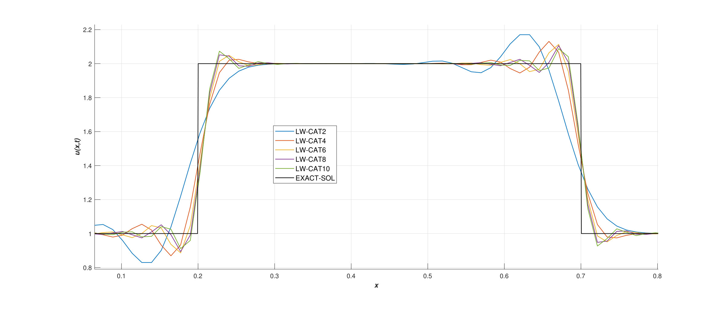 Figure 1
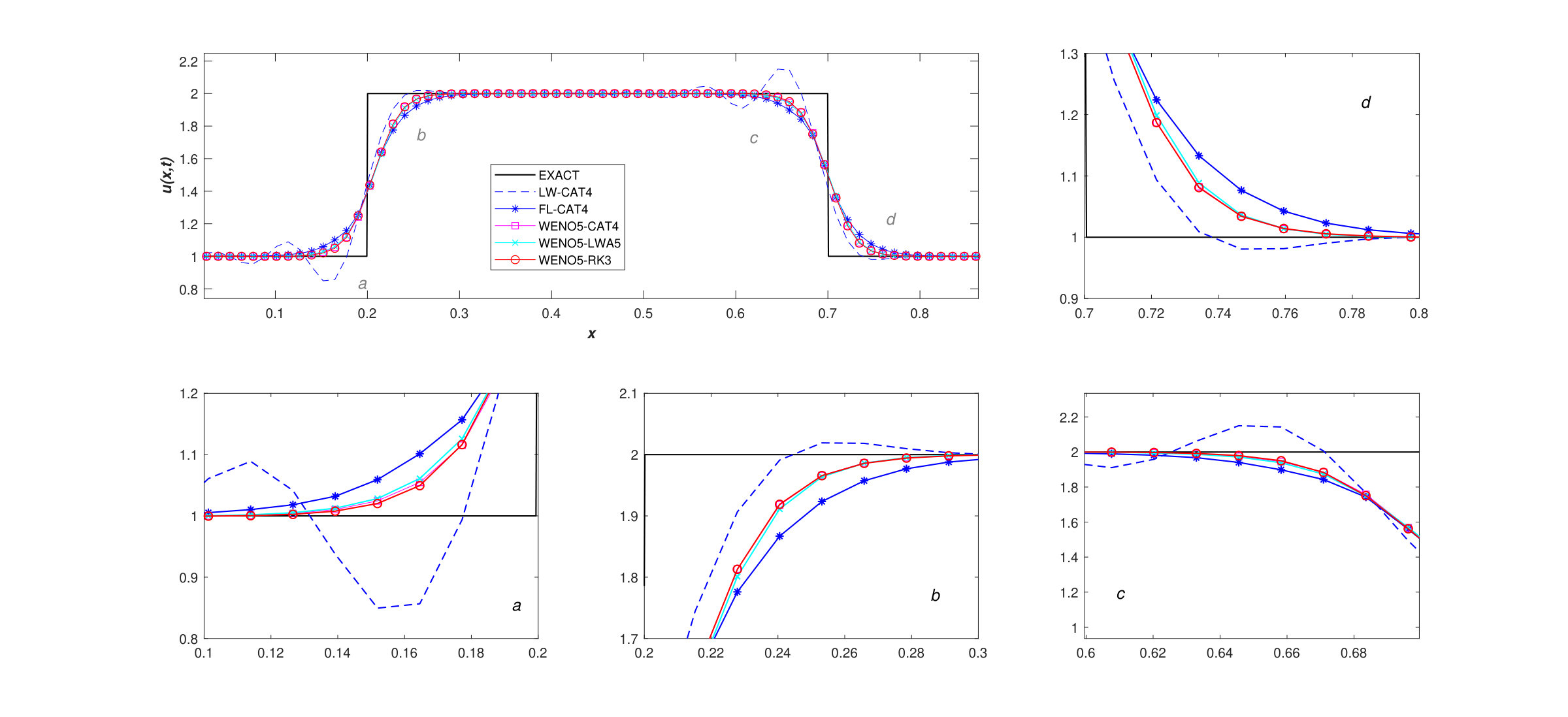 Figure 2
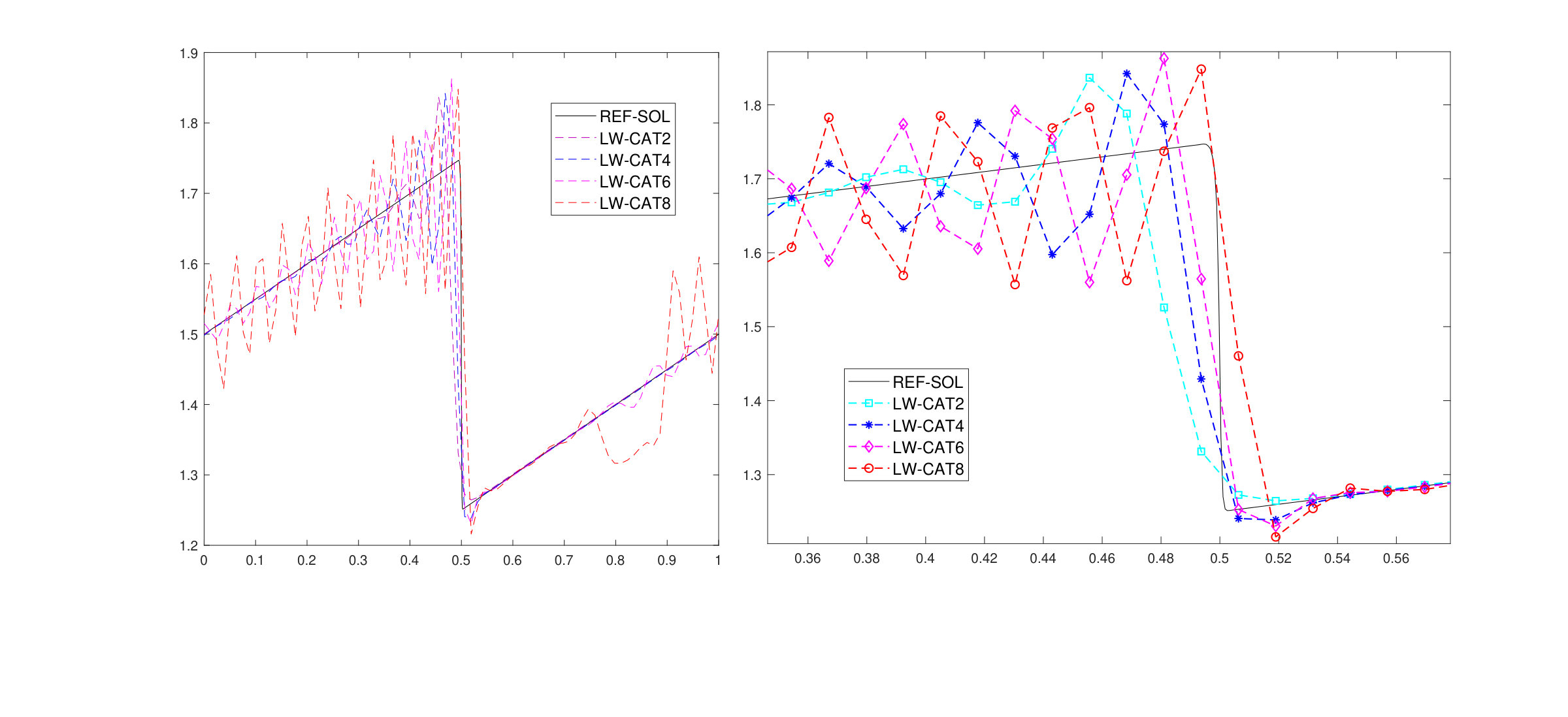 Figure 3
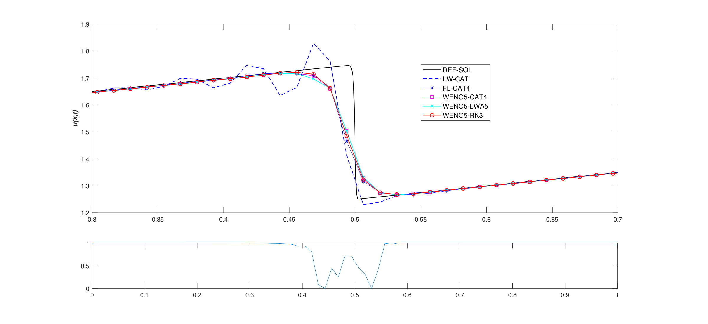 Figure 4
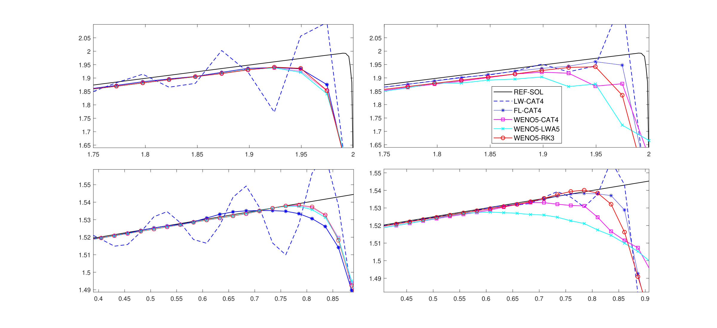 Figure 5
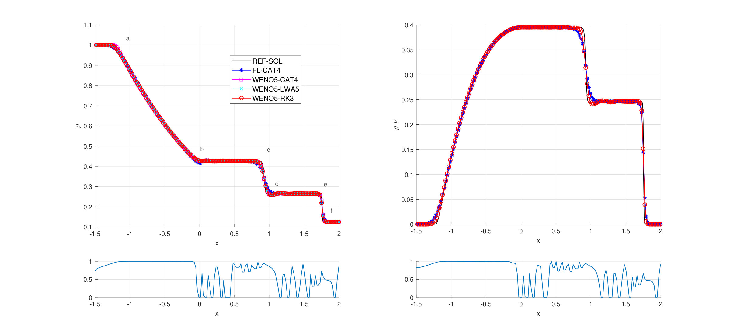 Figure 6
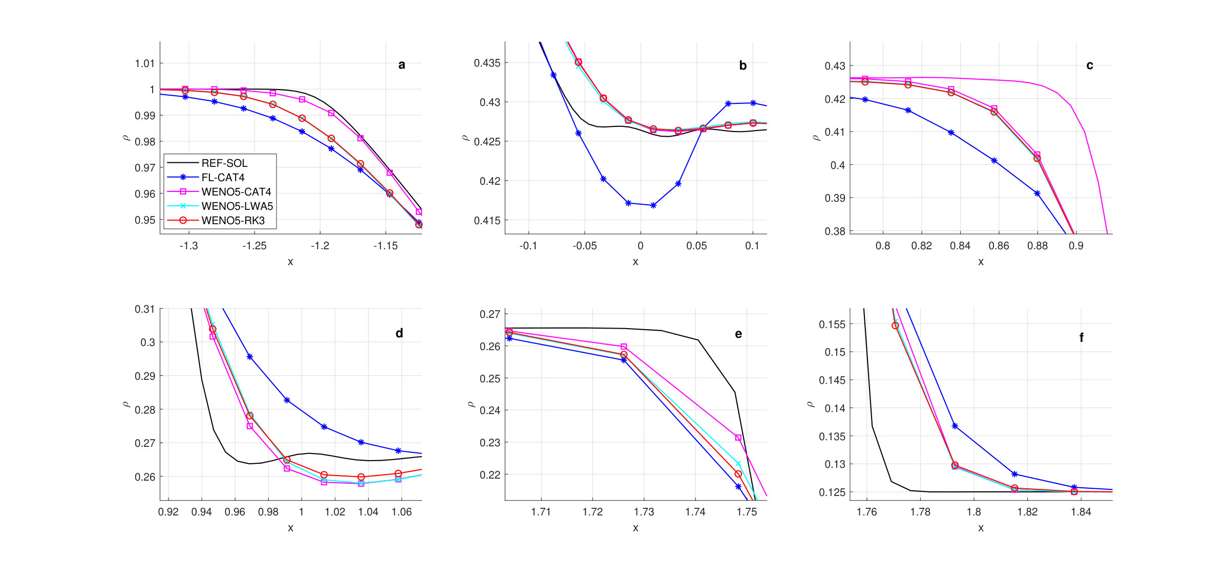 Figure 7
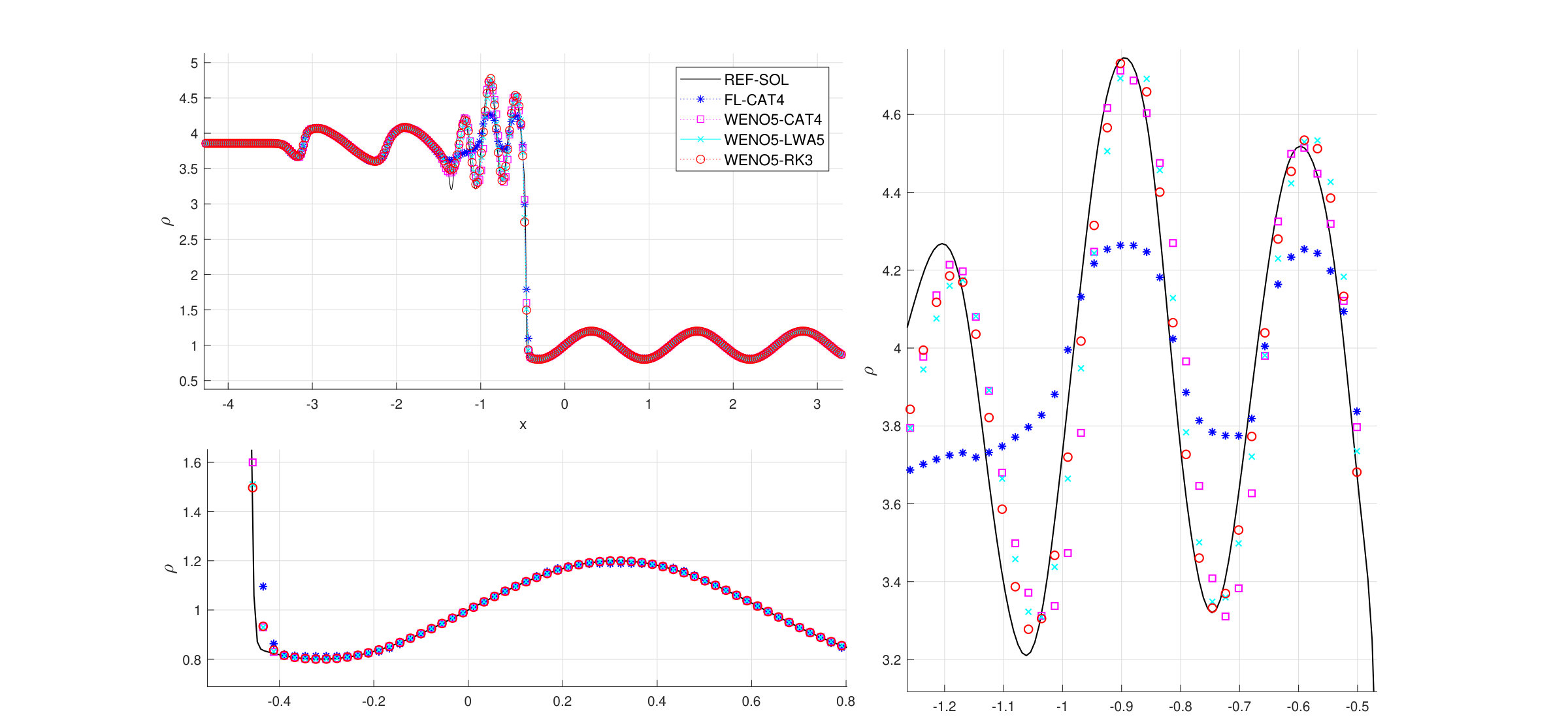 Figure 8
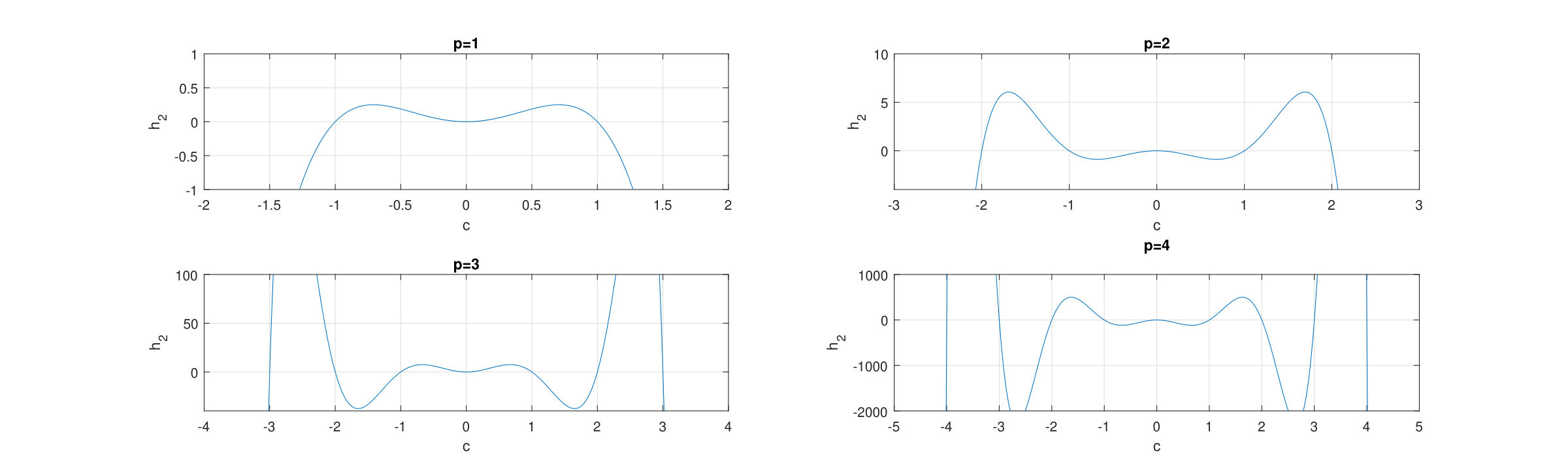 Figure 9
| 1 | 2 | 3 | 4 | |
|---|---|---|---|---|
| 1 | 2 | 4 | 6 | 8 |
| 2 | 2 | 4 | 6 | 8 |
| 3 | 2 | 4 | 6 | |
| 4 | 2 | 4 | 6 | |
| 5 | 2 | 4 | ||
| 6 | 2 | 4 | ||
| 7 | 2 | |||
| 8 | 2 |
| LW-CAT2 | LW-CAT4 | LW-CAT6 | LW-CAT8 | LW-CAT10 | |||||
|---|---|---|---|---|---|---|---|---|---|
| time | 1 | 2.98 | 7.72 | 18.87 | 42.66 | ||||
| flops | 1 | 1.61 | 2.51 | 3.69 | 5.16 |
| LW-CAT2 | LW-CAT4 | LW-CAT6 | ||||
|---|---|---|---|---|---|---|
| Error | Order | Error | Order | Error | Order | |
| 0.1053 | 3.68e-02 | 1.40e-02 | 7.88e-03 | |||
| 0.0526 | 6.84e-03 | 2.43 | 3.50e-05 | 8.64 | 4.25e-08 | 7.50 |
| 0.0263 | 1.70e-03 | 2.00 | 2.19e-06 | 4.00 | 6.49e-10 | 6.03 |
| 0.0132 | 4.27e-04 | 2.00 | 1.36e-07 | 4.00 | 9.89e-12 | 6.04 |
| 0.0066 | 1.06e-04 | 2.00 | 8.55e-09 | 4.00 | 1.53e-13 | 6.01 |
| 0.0033 | 2.66e-05 | 2.00 | 5.34e-10 | 4.00 | 2.64e-15 | 5.96 |
| WENO5-RK3 | WENO-LWA5 | |||
|---|---|---|---|---|
| Error | Order | Error | Order | |
| 0.1053 | 2.03e-03 | 5.44e-05 | ||
| 0.0526 | 6.06e-05 | 5.06 | 1.65e-06 | 5.04 |
| 0.0263 | 1.87e-06 | 5.02 | 5.04e-08 | 5.04 |
| 0.0132 | 5.83e-08 | 5.00 | 1.51e-09 | 5.05 |
| 0.0066 | 1.82e-09 | 5.00 | 4.41e-11 | 5.10 |
| 0.0033 | 5.65e-11 | 5.01 | 1.15e-12 | 5.25 |
| Nodes | LW-CAT4 | FL-CAT4 | WENO5-CAT4 | WENO5-LWA5 | ||
|---|---|---|---|---|---|---|
| 80 | 0.469 | 0.4702 | 0.5508 | 0.1998 | ||
| 160 | 0.8090 | 0.9668 | 0.9700 | 0.4616 | ||
| 320 | 1.9838 | 1.9908 | 2.0064 | 1.0346 |
| Nodes | FL-CAT4 | WENO5-CAT4 | |
|---|---|---|---|
| 80 | 0.2003 | 0.2078 | |
| 160 | 0.4024 | 0.5001 | |
| 320 | 1.0494 | 1.045 |
| LW-CAT2 | LW-CAT4 | LW-CAT6 | ||||
|---|---|---|---|---|---|---|
| Error | Order | Error | Order | Error | Order | |
| 0.1053 | 7.94e-03 | 9.01e-04 | 2.09e-04 | |||
| 0.0526 | 2.08e-03 | 1.93 | 6.13e-05 | 3.88 | 4.27e-06 | 5.62 |
| 0.0263 | 5.22e-04 | 1.99 | 3.89e-06 | 3.98 | 7.49e-08 | 5.83 |
| 0.0132 | 1.29e-04 | 2.01 | 2.44e-07 | 4.00 | 1.20e-09 | 5.96 |
| 0.0066 | 3.08e-05 | 2.00 | 1.51e-08 | 4.00 | 1.87e-11 | 6.00 |
| 0.0033 | 6.16e-06 | 2.00 | 8.76e-10 | 4.00 | 2.84e-13 | 6.00 |
| LW-CAT2 | LW-CAT4 | LW-CAT6 | ||||
|---|---|---|---|---|---|---|
| Error | Order | Error | Order | Error | Order | |
| 0.1053 | 3.34e-03 | 8.57e-04 | 5.49e-04 | |||
| 0.0526 | 8.82e-03 | 1.92 | 9.93e-05 | 3.11 | 3.53e-05 | 4.96 |
| 0.0263 | 2.28e-04 | 1.95 | 7.31e-06 | 3.76 | 1.01e-06 | 5.12 |
| 0.0132 | 5.69e-05 | 2.01 | 4.81e-07 | 3.93 | 1.94e-08 | 5.71 |
| 0.0066 | 1.35e-05 | 2.07 | 3.02e-08 | 3.99 | 3.21e-10 | 5.92 |
| 0.0033 | 2.71e-06 | 2.30 | 1.78e-09 | 4.08 | 4.99e-12 | 6.01 |
Peer Reviews
No public reviews on file for this paper yet. If you reviewed it on a platform where reviews are public (OpenReview, ICLR, NeurIPS, ICML), you can paste yours below so the community can read it here.
Videos
No videos yet. Explain this paper in a talk, walkthrough, or lecture? Add one.
Compact Approximate Taylor methods for systems of conservation laws.
H. [email protected], [email protected]
C. Parés [email protected], [email protected]
University of Málaga
Abstract
A new family of high order methods for systems of conservation laws are introduced: the Compact Approximate Taylor (CAT) methods. These methods are based on centered -point stencils where is an arbitrary integer. We prove that the order of accuracy is and that CAT methods are an extension of high-order Lax-Wendroff methods for linear problems. Due to this, they are linearly -stable under a condition. In order to prevent the spurious oscillations that appear close to discontinuities two shock-capturing techniques have been considered: a flux-limiter technique (FL-CAT methods) and WENO reconstruction for the first time derivative (WENO-CAT methods). We follow [14] in the second approach. A number of test cases are considered to compare these methods with other WENO-based schemes: the linear transport equation, Burgers equation, and the 1D compressible Euler system are considered. Although CAT methods present an extra computational cost due to the local character, this extra cost is compensated by the fact that they still give good solutions with CFL values close to 1.
1 Introduction
Lax-Wendroff methods for linear systems of conservation laws are based on Taylor expansions in time in which the time derivatives are transformed into spatial derivatives using the equations [5], [6],[12], [15]. The spatial derivatives are then discretized by means of centered high-order differentiation formulas. This procedure allows to derive numerical methods of order , where is an arbitrary integer, using a centered -point stencil that are -stable (a review on these methods will be presented in Section 2).
This paper focuses on the extension of Lax-Wendroff methods to nonlinear systems of conservation laws. This problem is closely related to the design of numerical schemes based on the methods of lines in which the time discretization is performed by means of Taylor or Approximate Taylor methods. Many authors have focused on the design of this type of methods that can be an alternative to time discretizations based on SSP Runge-Kutta methods [9] that lead to some stability restrictions for orders bigger than three. The main difficulty to extend Lax-Wendroff methods to nonlinear problems come from the transformation of time derivatives into spatial derivatives using the equations. A first strategy to do this is given by the Cauchy-Kovalevskaya (CK) procedure. In [9] this procedure has been used together with WENO reconstructions for the spatial discretization. The main benefit compared to RK time discretizations is that only one WENO reconstruction is needed at each spatial cell per time step. On the other hand, the main drawback comes from the fact that the CK procedure leads to expressions whose number of terms grow exponentially what implies high computational costs and difficult implementations. In [14] an alternative has been presented based on an Approximate Taylor (AT) method in which the time derivatives are approximated using high-order centered differentiation formulas combined with Taylor approximations in time that are computed in a recursive way. The resulting method is easy to implement and shows a good performance. Nevertheless AT schemes are not proper generalizations of Lax-Wendroff methods: they have -point stencils and worse linear stability properties than the original Lax-Wendroff methods. Nevertheless, they can be stabilized by using one WENO reconstruction per spatial cell and time step, like in [9] the resulting methods give good results under a condition typically.
In order to design numerical methods that are proper generalization of Lax-Wendroff methods, a compact variant of the AT procedure is introduced here: first, the conservative expression of the high-order Lax-Wendoff methods is considered; then, the derivatives appearing in the expression of the numerical flux are computed using -point differentiation formulas. This strategy lead to Compact Approximate Taylor (CAT) methods that have -point stencil and order of accuracy . They reduce to the Lax-Wendroff method when applied to a linear systems and thus they are linearly -stable under a condition. Nevertheless, the number of operations to perform a step is bigger than the original AT methods: this is due to the fact that the approximation of the time derivatives is local in the sense that they depend both on the point and on the stencil. However, this extra cost is compensated by better stability properties. As it happens with its linear counterpart, CAT methods lead to spurious oscillations near discontinuities. In order to cure them, two shock-capturing techniques are considered here: a flux-limiter technique and the use of a WENO reconstruction per cell and time step, as in [14] and [9].
This paper is organized as follows: in Section 2 a review of high order Lax-Wendroff methods for the linear transport equation is presented, including the study of the order and the -stability as well as the computation and properties of the coefficients. Section 3 is devoted to their extension to nonlinear problems: first the AT technique is recalled and then CAT methods are presented. We show that they reduce to Lax-Wendroff methods when applied to a linear problem and we analyze the order of accuracy. In Section 4 the techniques considered to cure the spurious oscillations near the discontinuities are presented. In Section 5 CAT methods are compared in a number of test cases with WENO-RK methods and AT methods. The linear transport equation, Burgers equation, and the 1D compressible Euler system are considered. Future developments and conclusions are drawn in Section 6.
2 The high-order Lax-Wendroff method for linear problems
Let us first consider the linear scalar equation:
[TABLE]
We consider the numerical method:
[TABLE]
where are the nodes of a uniform mesh of step ; is an approximation of the point value of the solution at at the time , where is the time step; is a natural number; ; and are the coefficients of the centered interpolatory formula of numerical differentiation based on a -point stencil:
[TABLE]
where represents the -th derivative of a one-variable function and . The expression of the numerical method is obtained by applying a Taylor expansion in time, and replacing time derivatives by space derivatives through the identities
[TABLE]
2.1 Formulas of numerical differentiation
Besides (3) the following family of interpolatory formulas based on a -point stencil will be used in this work:
[TABLE]
i.e. is the numerical differentiation formula that approximates the -th derivative at the point using the values of the function at the points . Observe that the coefficients, like in (3), do not depend on .
Given a variable , the following notation will be used:
[TABLE]
to indicate that the formulas are applied to the approximations of , , and not to its exact point values . In cases where there are two or more indexes, the symbol will be used to indicate with respect to which the differentiation is applied. For instance:
[TABLE]
Using this notation, the algorithm (2) writes as follows:
[TABLE]
Let us discuss some properties of the coefficients of the numerical differentiation formulas (3) and (5) and some relations between them that will be used in that follows. Since the coefficients are independent of and , we can consider, without loss of generality, the case , , :
[TABLE]
[TABLE]
Since (7) is exact for polynomials of degree , by applying the formula to , at , we get that the coefficients have to satisfy the equalities
[TABLE]
Analogously:
[TABLE]
[TABLE]
As it is well known, the coefficients are related to the Lagrange basis polynomials
[TABLE]
through the equalities:
[TABLE]
which allow us to write the Taylor expansion of centered at as follows:
[TABLE]
Proposition 1**.**
The coefficients of the formula (7), satisfy:
[TABLE]
- Proof.
(15) is deduced from the equality
[TABLE]
. Using (15) we get (16). (17) and (18) are deduced from (15) and (16).
Proposition 2**.**
For the following relations hold:
[TABLE]
- Proof.
Let us consider the formulas
[TABLE]
[TABLE]
that are exact for polynomials of degree . Let us consider now the formula
[TABLE]
If is a polynomial of degree , then (22) and (23) are exact for , furthermore
[TABLE]
where we have used that the formula
[TABLE]
is exact for polynomials of degree 1. Therefore, (24) coincide with (7). The proof is finished by writing (24) in the form
[TABLE]
and matching the weights.
Proposition 3**.**
Given , :
[TABLE]
- Proof.
The proof is similar to the one of the preceding in Proposition 2: consider the formula
[TABLE]
with
[TABLE]
check that it is exact for polynomials of degree ; write it in the form:
[TABLE]
and match its weights with those of (8).
2.2 Conservative form of (2)
From the proof of Proposition 2 we deduce an alternative form for (3):
[TABLE]
Using this form in (6), the numerical method (2) can be written as:
[TABLE]
with
[TABLE]
Using (11) it is straightforward to verify that is a consistent numerical flux, what proves that (2) is a conservative method.
2.3 Computation of the coefficients: an iterative algorithm
Notice that (9) constitutes a linear system with a Vandermonde matrix that can be used to compute . Nevertheless, as it is well-known, this system is ill-conditioned, so that it is recommendable to compute them by using an alternative algorithm: we adapt the recursive algorithm proposed in [3]. The following notation is adopted:
[TABLE]
Let us derive some recurrence formulas to compute the coefficients:
for .
From (12), we obtain
[TABLE]
Using then the Taylor expansions (14) in (29) we get
[TABLE] 2. 2.
with .
Substituting j=p in (12), we get
[TABLE]
and, using (14), we obtain:
[TABLE] 3. 3.
for . is used.
The algorithm is computed only once in increasing order of . The coefficients are computed using the algorithms described in [3],[2] and is obtained from .
2.4 Order of accuracy
Proposition 4**.**
The formula of numerical differentiation (3) has order of accuracy , with,
[TABLE]
- Proof.
Let be a function of class . Applying Taylor expansions and properties (9) and (17), we obtain:
[TABLE]
where
[TABLE]
Table 1 shows the order of (3) for different values of and .
Proposition 5**.**
*The discretization error of the numerical method (2) is of order . *
- Proof.
Let be a smooth enough solution of (1). Using Proposition 4 we obtain
[TABLE]
where (4) has been used.
As a consequence, the order of accuracy of (2) is . Therefore, the optimal combination of these parameters is . From now on, we shall assume that this relation holds.
2.5 Modified equation and stability
Taking into account that and (18), the local discretization error is as follows:
[TABLE]
[TABLE]
where is the polynomial of degree that interpolates the points
[TABLE]
Since is clearly an odd function, we finally obtain:
[TABLE]
Reasoning in a similar way, we get:
[TABLE]
where is the polynomial of degree that interpolates the points
[TABLE]
Using now (4), (35), and (36), the local discretization error can be written as follows:
[TABLE]
with
[TABLE]
Therefore, the numerical method solves with order the following modified equation
[TABLE]
where
[TABLE]
In order to study the stability, let us look for an elementary solution of (40) of the form
[TABLE]
where is complex number. The following equality has to be satisfied:
[TABLE]
Therefore:
[TABLE]
The numerical method is thus expected to be stable if the real part is negative, i.e.
[TABLE]
or, equivalently
[TABLE]
is a pair polynomial of degree such that
[TABLE]
Moreover, [math] is a double root of and are single roots. Analyzing the change of signs of , it can be easily checked that
[TABLE]
and thus (41) is satisfied if (see Figure 1). This argument shows that the stability of the method under the standard CFL condition can be formalized: extended details and a formal proof can be found in [8]. A study of the modified equation for the Lax Wendroff method can also be found in [13].
3 Extension to nonlinear problems
3.1 Approximate Taylor method
Following [14], instead of using the Cauchy-Kovaleskaya process to extend (27)-(28) to nonlinear problems
[TABLE]
we use the equalities
[TABLE]
To derive the expression of the numerical method, let us suppose that approximations
[TABLE]
are available. Then,
[TABLE]
being
[TABLE]
where, denotes the ceiling function.
Using these approximations to approximate the Taylor expansion, we obtain the method
[TABLE]
Equivalently, using (26), the numerical method can be written in conservative form (27) with numerical flux
[TABLE]
being
[TABLE]
Now, to compute the approximations , new Taylor expansions in time are used recursively as follows:
Compute .
- (a)
For :
- i.
Compute
[TABLE]
- ii.
Compute
[TABLE]
- iii.
Compute
[TABLE]
where
[TABLE]
Observe that Taylor expansions are used to approximate and once these approximations have been computed, the centered formula of numerical differentiation (3) is used to approximate the temporal derivatives.
This method is order , but it is not a generalization of (2) in the sense that this latter method is not recovered if . To see this, consider and : it can be easily checked that (45) writes as follows
[TABLE]
which is different from the standard Lax-Wendroff method: (45) is a -point method whose stability properties are worse than those of the standard Lax-Wendroff method. (see [6]).
3.2 Compact Approximate Taylor method
In order to prevent the increase of the stencil observed for Approximate Taylor methods, we consider a modification based on the conservative form of the method. The numerical flux will be computed using only the approximations
[TABLE]
so that the values used to update are only those of the centered -point stencil, like in the linear case. In fact, we will show that this modification is a proper generalization of the Lax-Wendroff method for linear problems.
In order to be able to compute the numerical fluxes using only (49), for every we will compute local approximations of
[TABLE]
that will be represented by
[TABLE]
These approximations are local in the sense that , does not imply that . Once these approximations have been computed, the numerical flux is given by
[TABLE]
with
[TABLE]
Now, given , to compute the approximations , new Taylor expansions in time are used recursively as follows:
Compute
- (a)
For :
- i.
Compute
[TABLE]
where
[TABLE]
- ii.
Compute
[TABLE]
- iii.
Compute
[TABLE]
with
[TABLE]
Notice that, unlike the Approximate Taylor methods (in which all the derivatives were approximated using the centered -point formula), in this algorithm the stencil is used for the space derivatives and the stencil for the time derivative.
Theorem 1**.**
*The compact approximate Taylor method reduces to (2) when . *
- Proof.
For we have:
[TABLE]
where (10) has been used. On the other hand:
[TABLE]
where (25) has been used. By recurrence:
[TABLE]
Next,
[TABLE]
where (25) has been used. Finally,
[TABLE]
what is the numerical flux (28) corresponding to (2), as we wanted to prove.
As a consequence, we obtain that the compact approximate Taylor method is linearly stable (in the sense) under the usual CFL condition
[TABLE]
Theorem 2**.**
*The compact approximate Taylor method is order . *
- Proof.
Let us perform a step of the method starting from the point values at time , , of a smooth enough exact solution. We assume that remains constant.
First we have:
[TABLE]
Next:
[TABLE]
where
[TABLE]
is the first order Taylor polynomial in time of in . Then
[TABLE]
where (10) has been used. This result can be extended by induction to every between 1 and as follows:
[TABLE]
Using this equality we get:
[TABLE]
Remark: In the Approximate Taylor method proposed in [14] the derivatives are computed by applying the -point centered differentiation formula for first derivatives to , where is given by (44): notice that decreases as increases. The same reduction of the stencil used to compute could be applied here, what would allow us to reduce the number of computations while preserving the overall order of accuracy. Nevertheless, the resulting method will not be an extension of the linear Lax-Wendroff method. On the other hand, the CPU reduction will be not significant.
3.3 Example: Fourth order compact approximate Taylor method
Since the method is conservative, we will only show in detail how to compute the numerical flux (50) and, to do this, it is enough to specify how to compute
[TABLE]
The procedure is as follows:
: First the assignment
[TABLE]
is done and then:
[TABLE]
- 2.
: The first order time derivatives of at the nodes are approximated by applying the corresponding differentiation numerical formula to :
[TABLE]
Next first order Taylor expansions are used to approximate the values of the flux sixteen space-time local nodes: for
[TABLE]
Then, the first order time derivates of the flux at the nodes are approximated by applying the corresponding differentiation numerical formula to :
[TABLE]
Finally;
[TABLE]
- 3.
: the second order time derivatives at the nodes are approximated by
[TABLE]
Second order Taylor expansions are used to compute the fluxes at the sixteen nodes in the space-time mesh: for
[TABLE]
Next, compute
[TABLE]
And finally;
[TABLE]
- 4.
: the third order time derivatives at the nodes are approximated by
[TABLE]
Compute the approximations of the fluxes: for
[TABLE]
Next, compute:
[TABLE]
Finally;
[TABLE]
If , then:
[TABLE]
which coincides with the numerical flux of the fourth order Lax-Wendroff in conservative form.
4 Shock-capturing techniques
Although the Compact Approximate Taylor methods are linearly stable in the sense under the usual -1 condition, they may produce strong oscillations close to a discontinuity of the solution. The goal of this section is to modify the numerical method to avoid these oscillations. Two different techniques are considered here:
4.1 FLUX LIMITER-CAT methods
We consider the numerical method (27) with
[TABLE]
where is a first order robust numerical flux, is given by (50), and is the flux limiter function, see [4] [7], [12]. We consider here
[TABLE]
where is the van Albada second version flux limiter:
[TABLE]
and
[TABLE]
where, is an estimate of the wave speed.
4.2 WENO-CAT methods
Following [9] WENO reconstructions of the flux are used to stabilize the method. The only differences with the algorithm described in Section 3.2 are the computation of , that is now performed as follows:
[TABLE]
where denotes the WENO flux splitting, reconstructions at of the flux function described in [10]. The expression of the numerical flux is then given by:
[TABLE]
4.3 Systems of conservation laws
Although the methods have been described in the scalar case for simplicity, they can be easily applied to systems using vector notation.
5 Numerical Experiments
In this section we apply to some scalar conservation laws and to the 1D Euler equation the following numerical methods:
LW-CAT: Compact Approximate Taylor method of order (space and time).
- 2.
FL-CAT: Compact Approximate Taylor method of order with flux limiter technique. The first order methods considered are Lax-Friedrich for scalar problems and HLL for systems.
- 3.
WENO-CAT: Compact Approximate Taylor method of order with WENO reconstructions of order to compute .
- 4.
WENO-RK: WENO method of order for the space discretization and TVD-RK for the time discretization, see [10].
- 5.
WENO-LWA: Approximate Taylor method of order with WENO reconstructions of order to compute , see [14].
5.1 Linear transport equation
We consider first (1) with , in the space interval , with initial condition
[TABLE]
and periodic boundary conditions. A uniform mesh with points is considered and the LW-CAT method (that, in this case, coincides with the Lax-Wendroff method) is applied for .
Numerical simulations are shown in Figure 2: the stability of the scheme and the appearance of oscillations near the discontinuities can be observed. Next, we apply to the same problem LW-CAT4, FL-CAT4, WENO5-CAT4, WENO5-RK3, and WENO5-LWA5 methods. A general view is shown in Figure 3 together with a zoom of the area of interest. As it can be observed, the results given by WENO5-CAT4, WENO5-RK3 and WENO5-LWA5 are almost identical. Nevertheless, as it will be seen in the next test problem, WENO5-CAT4 still gives good results for CFL close to one, what is not the case for WENO5-RK3 or WENO5-LWA5.
Using the algorithm in Section 3.2 CAT methods are easily extended to any order, nevertheless, this involves a significant increase of the CPU time simulation and flops (number of operations required), that should be considered, see Table 2.
Finally, we consider (1) in the space interval with initial condition,
[TABLE]
and periodic boundary conditions. Table 3 shows the error and the empirical order for LW-CAT2, LW-CAT4, LW-CAT6, and Table 4 for WENO5-RK3 and WENO5-LWA5 which coincides in all cases with the theoretical one. For smooth solutions WENO-CATq and FL-CATq reduce to the corresponding LW-CATq, so that the accuracy test is not necessary.
5.2 Burgers equation
We consider Burgers equation, i.e. (42) with
[TABLE]
When CAT methods are applied to approximate a discontinuous solution of this nonlinear problem, the oscillations appearing close to the shocks tend to grow and to spoil the numerical solution. Nevertheless, it is still possible to apply these methods by reducing the parameter (the reduction increases with ): for instance, Figure 4 shows the results obtained with CAT-LW2, and , respectively, with initial conditions (62).
Next, the same test problem is solved using LW-CAT4, FL-CAT4, WENO5-RK3 and WENO5-LWA5 methods. Using we obtain numerical solutions without spurious oscillations for all the methods. Figure 5 shows a general view of solutions and the van Albada flux limiter function on every inter cell. In Figure 6 the results are compared with those obtained with . From Figures 5, 6 we can conclude:
- (a)
LW-CAT4 show oscillations near the discontinuities, but it is stable.
- (b)
FL-CAT4 is very diffusive near to the discontinuities, due to the selected first order accurate flux limiter function.
- (c)
WENO5-CAT4, WENO5-LWA4 and WENO5-RK3 show good results, stable and essentially the same values.
- 2.
- (a)
LW-CAT4: the amplitude of oscillations increases near the discontinuities. However, they remain stable.
- (b)
FL-CAT4: conversely to the previous condition, it shows acceptable solutions near the discontinuities.
- (c)
WENO5-CAT4 ,WENO5-LWA5 and WENO5-RK3 : slight oscillations appear near the discontinuities at the beginning of the simulations. Nevertheless, as the time increases, these oscillations tend to dismiss and the result remains acceptable and stable for WENO5-CAT4 while the solutions given by WENO5-LWA5 is very diffusive and the one given by WENO5-RK3 is overdamped.
Although FL-CAT4 shows better results for bigger , it fails in smooth regions close to critical points and for systems (as it will be seen in Euler 1D equation). For , WENO5-LWA5 is faster than CAT methods (in the computational cost sense): a comparsion is shown in Table 5. However, we can obtain good solutions for CAT methods using and obtain similar CPU time computation, see Table 6.
In order to study the order of convergence, we consider again initial condition (63) and periodic boundary conditions. A reference solution at time s (when the solution is still smooth) is obtained with WENO5-RK3 using a fine grid of nodes. The errors and the empirical order are shown in Table 7: the numerical results verify the theoretical analysis.
5.3 1D Euler Equation
We solve the Euler equation for gas dynamics
[TABLE]
with
[TABLE]
where is the density, the velocity, the total energy per unit volume, and the pressure. We assume an ideal gas with the equation of state,
[TABLE]
being the ratio of specific heat capacities of the gas taken as 1.4 and is the internal energy per unit mass given by:
[TABLE]
We consider the space interval with the initial condition:
[TABLE]
and periodic boundary conditions. For this test we take and s. We use a fine grid with -point mesh to compute LW-CAT8 as a reference solution. The results in Table 8 support the theoretically obtained accuracy.
Finally, two tests involving discontinuities are considered:
The Sod Shock tube problem. The initial condition is given by:
[TABLE]
Here, , , s, and outflow boundary conditions are considered at both sides. For details of this problem see [11]. We compare FL-CAT4, WENO5-CAT4, WENO5-LWA5 and WENO5-RK3 using points. A reference solution is computed with WENO5-RK3 using a -point mesh. The flux limiter function is computed for every variable.
While all numerical solutions show stable and similar values over smooth regions (see Figure 7), the quality is different in the interest regions (a,b,c,..,f): an enlarged view of them can be seen in Figure 8. In the figure we can observe that the solution given by FL-CAT4 is the most diffusive one (due to the condition ) and that WENO5-LWA5 and WENO5-RK3 give essentially the same results. WENO5-CAT4 achieves some improvements, specially in a,c and d.
The Shu-Osher problem. The initial condition is given by:
[TABLE]
We consider the space interval , and time s. For details see [10] test 8. We compare FL-CAT4, WENO5-CAT4, WENO5-LWA5 and WENO5-RK3 using - point mesh and a reference solution computed with WENO5-RK3 using a -point mesh.
Again, all solutions are closely similar and near to the reference solution with exception of FL-CAT4.
6 Conclusions
In this work, first a review of high order Lax-Wendroff methods for the linear transport equation has been presented, including the study of the order and the -stability as well as the computation and properties of the coefficients. Next, an extension to nonlinear conservation laws has been introduced with arbitrary even order of accuracy, the so-called Compact Approximate Taylor (CAT) methods. Unlike previous applications of Taylor methods to conservation laws, CAT methods have -point centered stencils, like Lax-Wendroff methods for linear problems. Moreover, since they inherit the stability properties of Lax-Wendroff methods, they are linearly -stable under a CFL-1 condition. In order to prevent the spurious oscillations that appear close to discontinuities two shock-capturing techniques have been considered: a flux-limiter technique (FL-CAT methods) and WENO reconstruction for the first time derivative (WENO-CAT methods). We follow [14] in the second approach.
These new methods have been compared in a number of test cases with WENO-RK methods (Finite Differences WENO reconstructions in space, TVD-RK in time) and with the WENO-LW methods introduced in [14] (Finite Differences WENO reconstruction for the first time derivative, Approximate Taylor in time). The linear transport equation, Burgers equation, and the 1D compressible Euler system have been considered.For all the numerical methods work correctly, and the results obtained with all the methods using WENO reconstructions are similar, while the FL-CAT method is more diffusive as expected. Nevertheless, CAT methods are more expensive in computational time and number of operations due to its local character (FL-CAT is less expensive than WENO-CAT as reconstructions are avoided). However, the extra computational cost of CAT methods is compensated by the fact that they still give good solutions with CFL values close to 1.
Future developments include:
Parallel implementation.
- 2.
Use of fast WENO reconstructions: see [1]
- 3.
Order adaptive CAT methods based on smooth indicators.
- 4.
Application to systems of balance laws.
- 5.
Extension to multidimensional problems.
7 Acknowledgements
“This project has received funding from the European Union’s Horizon 2020 research and innovation program, under the Marie Sklodowska-Curie grant agreement No 642768”.
The reference list from the paper itself. Each links out to its DOI / PubMed record.
- 1[1] A. Baeza, R. Bürger, P. Mulet, and D. Zorío. On the efficient computation of smoothness indicators for a class of weno reconstructions. CIMA Pre-Publicación 2018-37 , 2018.
- 2[2] B. Fornberg. Classroom note:calculation of weights in finite difference formulas. SIAM Review , 40(3):685–691, 1998.
- 3[3] Bengt Fornberg. Generation of finite difference formulas on arbitrarily spaced grids. Mathematics of Computation , 51(184):699–706, 1988.
- 4[4] Friedemann Kemm. A comparative study of tvd-limiters—well-known limiters and an introduction of new ones. International Journal for Numerical Methods in Fluids , 67(4):404–440, 2010.
- 5[5] Peter Lax and Burton Wendroff. Systems of conservation laws. Communications on Pure and Applied Mathematics , 13(2):217–237, 1960.
- 6[6] Randall Le Veque. Finite Difference Methods for Ordinary and Partial Differential Equations: Steady-State and Time-Dependent Problems (Classics in Applied Mathematics Classics in Applied Mathemat) . Society for Industrial and Applied Mathematics, Philadelphia, PA, USA, 2007.
- 7[7] Randall J. Le Veque. Finite Volume Methods for Hyperbolic Problems . Cambridge Texts in Applied Mathematics. Cambridge University Press, 2002.
- 8[8] Jiequan Li and Zhicheng Yang. The von neumann analysis and modified equation approach for finite difference schemes. Applied Mathematics and Computation , 225:610 – 621, 2013.