Minimal Lipschitz and $\infty$-Harmonic Extensions of Vector-Valued Functions on Finite Graphs
Miroslav Ba\v{c}\'ak, Johannes Hertrich, Sebastian Neumayer, Gabriele, Steidl

TL;DR
This paper investigates minimal Lipschitz and $ abla$-harmonic extensions of vector-valued functions on finite graphs, showing convergence of $p$-Laplacian solutions to these extensions and exploring their applications in image inpainting.
Contribution
It establishes the equivalence of lex and L-lex minimal extensions, proves convergence of $p$-Laplacian solutions to minimal Lipschitz extensions, and connects these concepts to iterative filters and $ abla$-Laplacians.
Findings
Lex and L-lex minimal extensions are identical.
Solutions of graph $p$-Laplacians converge to minimal Lipschitz extensions as $p o abla$.
Iterative algorithms for $ abla$-Laplacians are proven to converge.
Abstract
This paper deals with extensions of vector-valued functions on finite graphs fulfilling distinguished minimality properties. We show that so-called lex and L-lex minimal extensions are actually the same and call them minimal Lipschitz extensions. Then we prove that the solution of the graph -Laplacians converge to these extensions as . Furthermore, we examine the relation between minimal Lipschitz extensions and iterated weighted midrange filters and address their connection to -Laplacians for scalar-valued functions. A convergence proof for an iterative algorithm proposed by Elmoataz et al.~(2014) for finding the zero of the -Laplacian is given. Finally, we present applications in image inpainting.
Click any figure to enlarge with its caption.
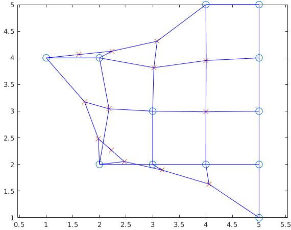 Figure 1
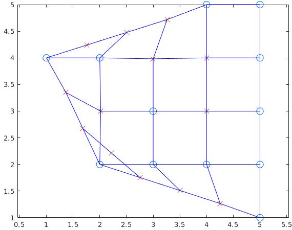 Figure 2
 Figure 3
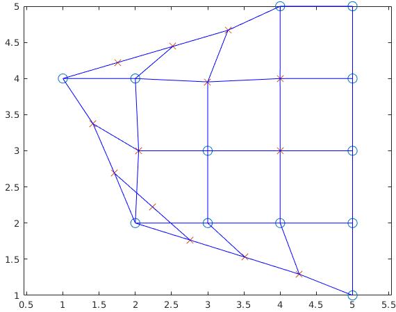 Figure 4
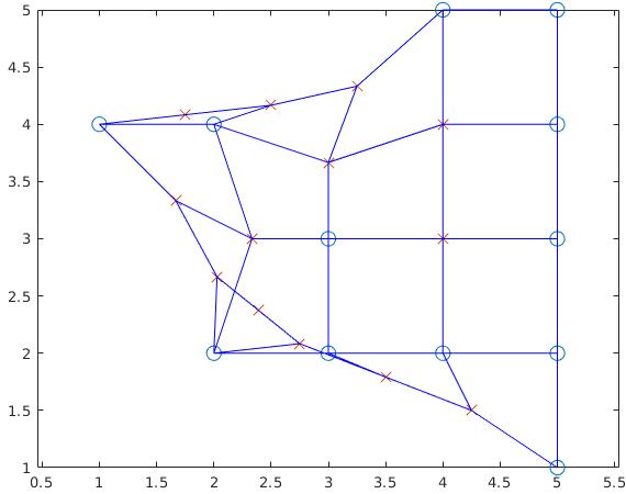 Figure 5
 Figure 6
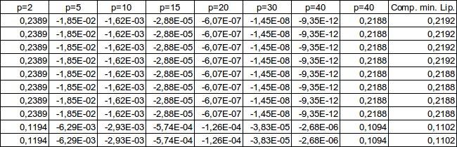 Figure 7
 Figure 8
 Figure 9
 Figure 10
 Figure 11
 Figure 12
 Figure 13
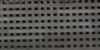 Figure 14
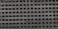 Figure 15
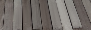 Figure 16
 Figure 17
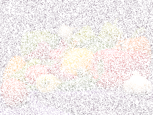 Figure 18
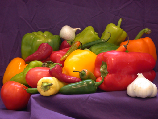 Figure 19
 Figure 20
 Figure 21
 Figure 22
 Figure 23
 Figure 24
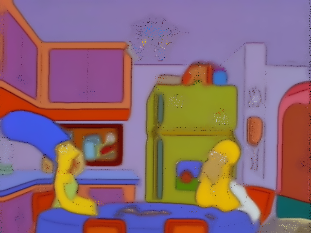 Figure 25
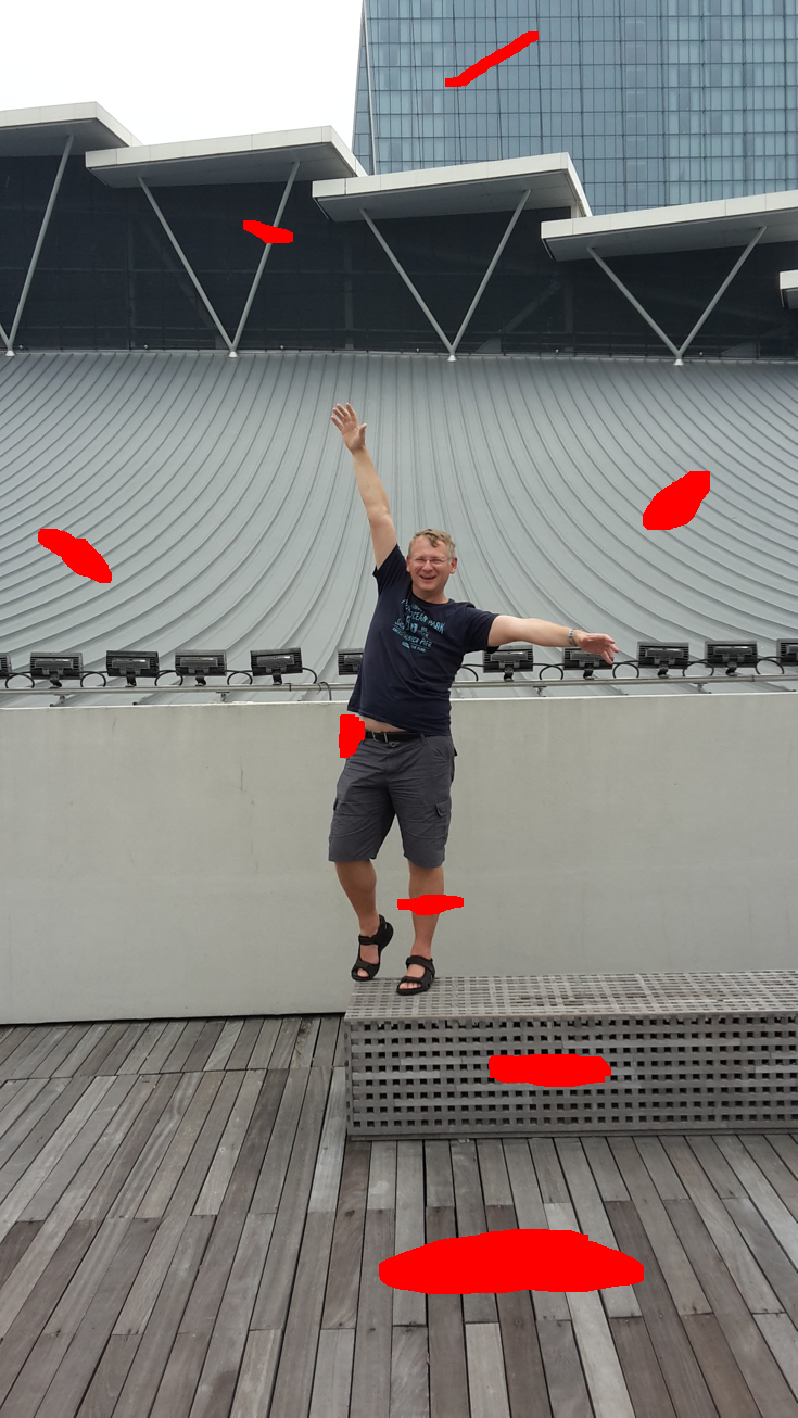 Figure 26
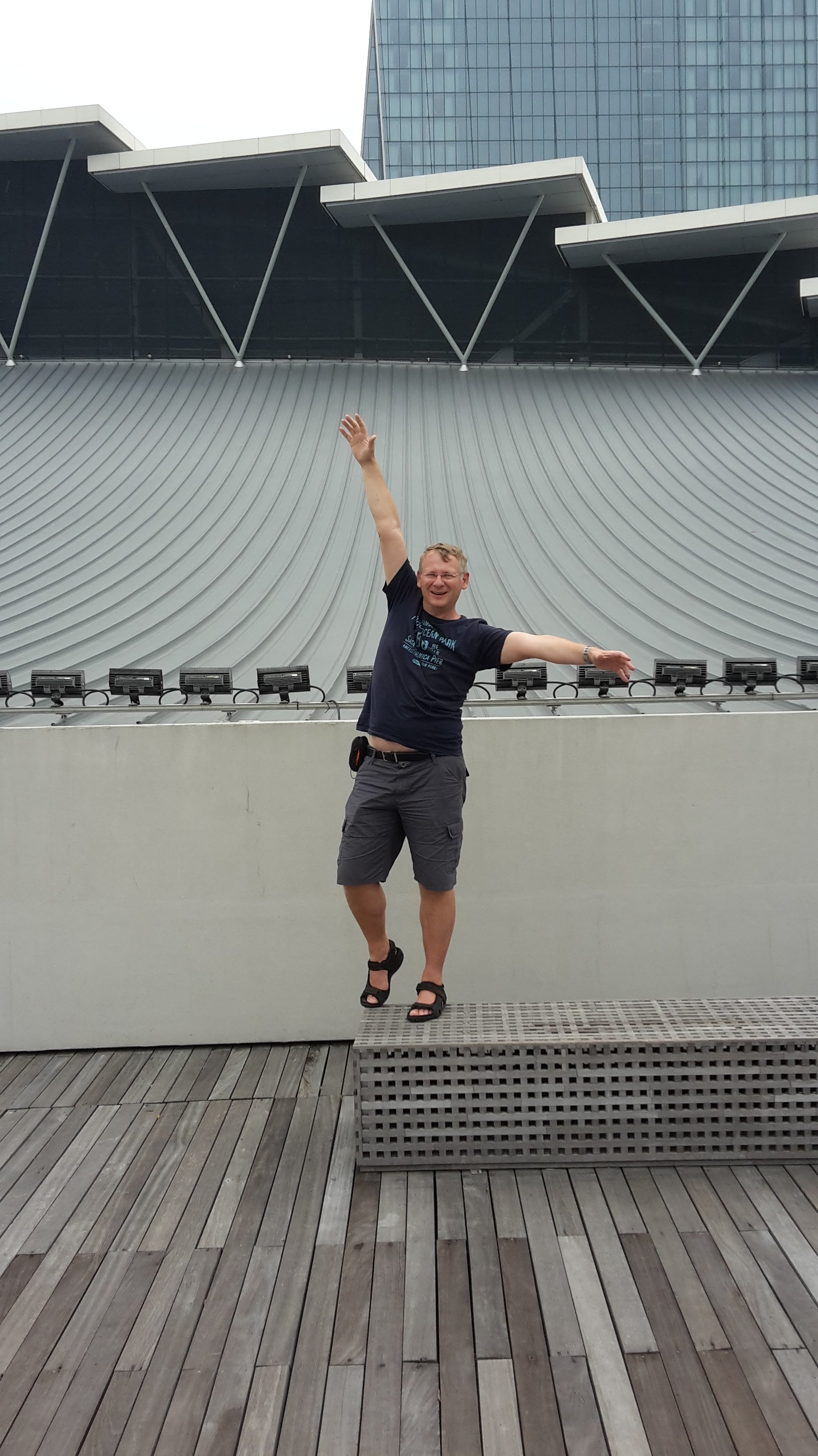 Figure 27
 Figure 28
 Figure 29
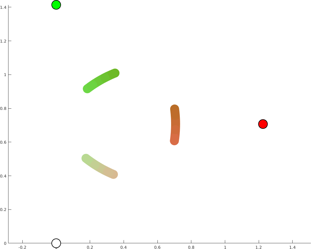 Figure 30
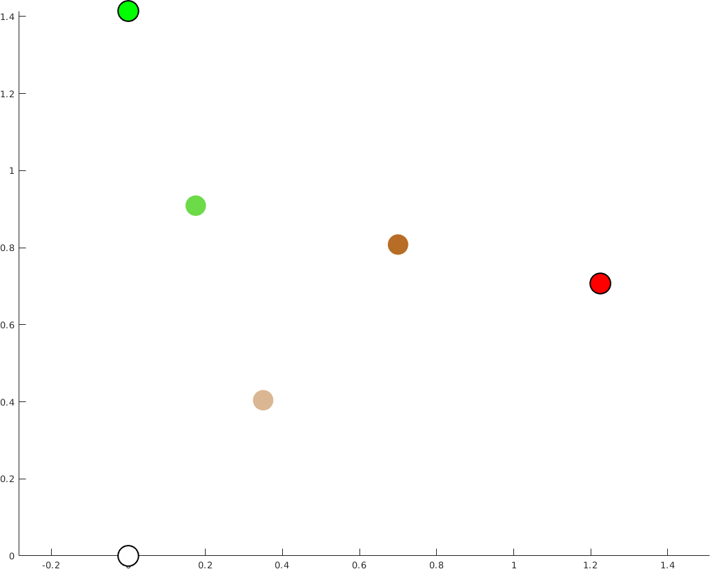 Figure 31
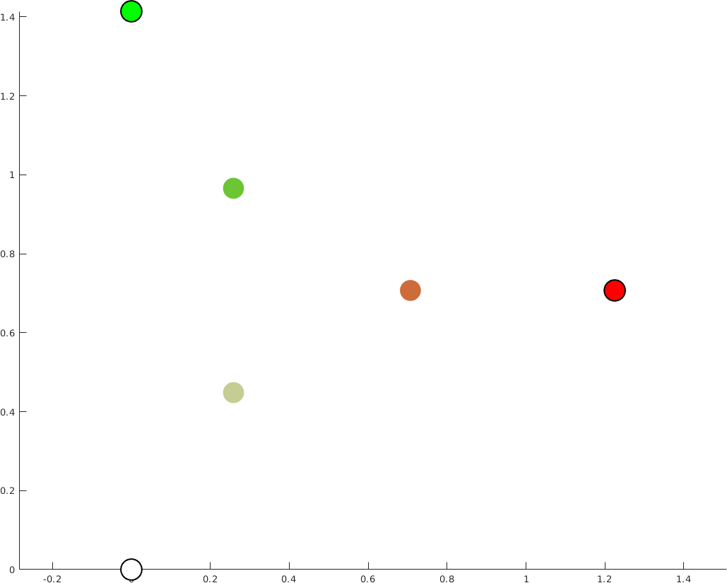 Figure 32
Peer Reviews
No public reviews on file for this paper yet. If you reviewed it on a platform where reviews are public (OpenReview, ICLR, NeurIPS, ICML), you can paste yours below so the community can read it here.
Code & Models
Videos
No videos yet. Explain this paper in a talk, walkthrough, or lecture? Add one.
Taxonomy
TopicsSparse and Compressive Sensing Techniques · Advanced Mathematical Modeling in Engineering · Topological and Geometric Data Analysis
\setkomafont
sectioning \setkomafonttitle
Minimal Lipschitz and -Harmonic Extensions
of Vector-Valued Functions on Finite Graphs
Miroslav Bačák
Max Planck Institute for Mathematics in the Sciences, Inselstr. 22, 04103 Leipzig, Germany, [email protected]
Johannes Hertrich
Department of Mathematics, Technische Universität Kaiserslautern, Paul-Ehrlich-Str. 31, 67663 Kaiserslautern, Germany, {jhetric,neumayer,steidl}@mathematik.uni-kl.de
Sebastian Neumayer
Department of Mathematics, Technische Universität Kaiserslautern, Paul-Ehrlich-Str. 31, 67663 Kaiserslautern, Germany, {jhetric,neumayer,steidl}@mathematik.uni-kl.de
Gabriele Steidl
Department of Mathematics, Technische Universität Kaiserslautern, Paul-Ehrlich-Str. 31, 67663 Kaiserslautern, Germany, {jhetric,neumayer,steidl}@mathematik.uni-kl.de
Fraunhofer ITWM, Fraunhofer-Platz 1, 67663 Kaiserslautern, Germany
Abstract
This paper deals with extensions of vector-valued functions on finite graphs fulfilling distinguished minimality properties. We show that so-called and minimal extensions are actually the same and call them minimal Lipschitz extensions. Then we prove that the solution of the graph -Laplacians converge to these extensions as . Furthermore, we examine the relation between minimal Lipschitz extensions and iterated weighted midrange filters and address their connection to -Laplacians for scalar-valued functions. A convergence proof for an iterative algorithm proposed by Elmoataz et al. (2014) for finding the zero of the -Laplacian is given. Finally, we present applications in image inpainting.
Keywords: -Laplacian, -Laplacian, graph Laplacian, -harmonic extension, absolutely minimal Lipschitz extension, midrange filter, image inpainting, nonlocal techniques
1 Introduction
In this paper, we study an -harmonic variant of the Dirichlet problem for vector-valued functions defined on finite graphs. To be more specific, we assume that a vector-valued function is given on a subset of the vertex set (“boundary”) and our goal is to extend this function onto the whole vertex set so that the extension is -harmonic. However, as observed by [38], -harmonic extensions of vector-valued functions on finite graphs are not uniquely determined. To overcome this non-uniqueness issue they introduced the stronger notion of tight extensions and proved that such extensions exist and are unique. In the present paper, we approach these extensions from a different point of view and call them minimal Lipschitz extension, since its local Lipschitz constant (“oscillation”) is in some sense optimal. We therefore aim at finding a solution to the above boundary problem which is minimal Lipschitz.
In [38, Section 2] an algorithm for computing these minimal Lipschitz extensions in the scalar-valued case was presented. To the best of our knowledge there exists no meaningful algorithm for computing minimal Lipschitz extensions of vector-valued functions and it is our goal to address their approximation in the present paper. Along the way we also clarify various aspects concerning minimal Lipschitz extensions and their relations to other concepts including iterated midrange filters, minimizers of -energy functionals, -Laplacians and -Laplacians.
The topic of minimal Lipschitz extensions on graphs appears in various subfields of mathematics and computer science from different points of view and with different notations. These areas include approximation theory [12], discrete mathematics/graph theory [32], data and image processing [3, 14, 16, 39] including manifold-valued data [5], and mathematical morphology [37] to mention only a few. While many results on minimal Lipschitz extensions are available for scalar-valued functions, the vector-valued case has been less studied.
We work with weighted graphs which turns out to be crucial for the applications in image processing. Indeed, in Section 8, we present applications of minimal Lipschitz extensions for inpainting of vector-valued images which rely upon representing the image under consideration as a function on an appropriate weighted graph which is obtained by nonlocal patch-based techniques.
As a matter of fact, [38] define tight extensions also for functions defined on a bounded, open, connected subset . This is closely related to absolutely minimizing Lipschitz extensions (AMLE) and therefore also to -harmonic functions. Indeed, [22], stimulated by the work [1], proved that for , the boundary-value problem
[TABLE]
with the -Laplacian defined by
[TABLE]
has a unique viscosity solution . [11] showed its equivalence to the AMLE of . In connection with image interpolation algorithms and elliptic partial differential operators, AMLEs were studied by [10] inspired by the work of [9]. The operator was considered, e.g., for comparisons of image compression algorithms in [17, 36]. Even though we are aware of the existence of this deep theory of Lipschitz extensions in we focus exclusively on functions defined on finite graphs in the present paper. For more information on the continuous case, the interested reader is also referred to the recent papers [23, 24, 28] and the references therein.
This paper is organized as follows. After fixing the notation in Section 2, we introduce and minimal extensions in Section 3 and prove that they actually coincide. In Section 4, we show that the minimizers of the grouped -energy functionals converge to these extensions as . Section 5 deals with the relation between iterated midrange filters and minimal Lipschitz extensions. In Section 6, we consider -Laplacians for scalar-valued functions and provide a convergence proof for an iterative algorithm of [15]. Section 7 contains finer analyses of the numerical algorithms. Finally, Section 8 shows applications in image inpainting. Preliminary results of the present paper are contained in the conference paper [20].
2 Preliminaries
Let be a finite, undirected, connected, weighted graph with weight function We use the usual notation for Let and assume if . Denote and . We also suppose that if and only if Since the graph is not directed, the weights are symmetric, that is, . Finally, we suppose that for .
The set of functions is denoted by . For a given function , let denote those functions with , which are called extensions of .
The 2--norm, for and the --norm are defined for as \left\lVert x\right\rVert_{2,p}\coloneqq\bigl{(}\sum_{i=1}^{n}|x_{i}|^{p}\bigr{)}^{1/p}, and , where denotes the Euclidean norm of . For , we have just the usual -norms which we denote by , for .
In [18] the discrete gradient operator was introduced by where Let be given. For , we are interested in the anisotropic energies of the -Laplacians
[TABLE]
The functionals , for are strictly convex and hence they have a unique global minimum . Besides , the functional
[TABLE]
was considered by [38]. This functional is not strictly convex for , but has nevertheless a unique minimizer of ; see [19]. In contrast to or , for , the functional has in general many minimizers. In this paper, we want to accent minimizers of with distinguished properties.
Using -convergence arguments, it is not hard to show that every cluster point of the sequence of the minimizers of , resp. is a minimizer of . For convenience, we add the short proof.
Lemma 2.1**.**
Every cluster point of the sequence of minimizers of is a minimizer of . The same holds true for the minimizers of
Proof.
Recall that the -norms satisfy
[TABLE]
In particular, as uniformly on bounded sets and the convergence is monotone. These properties are inherited by the convergence as . This implies that -converges to as and we obtain the desired results since the functionals and have the same minimizers. Similar arguments can be applied for the functional . ∎
3 Minimal Lipschitz Extensions
Let again be a nonempty subset of the vertices of the graph and let We start by recalling the definitions of two types of minimal extensions of and we then show in Theorem 3.2 below that they actually coincide. For , let
[TABLE]
and be the vector with entries in nonincreasing order. Note that we count the entries only once. For , define
[TABLE]
and the vector with entries in nonincreasing order. Denoting by the lexicographical ordering, a function is called
- (i)
minimal extension (of ) if for every , and 2. (ii)
minimal extension (of ) if for every .
The first notation can be found for instance in [26]. The minimal extension was called tight extension in the paper [38].
The existence of minimal extensions in the non-weighted case was shown in [38, Theorem 1.2]. The existence in the weighted setting as well as for minimal extensions can be proved similarly; see [19]. By definition we clearly have , where the subscript denotes the coordinate index. In this section, we want to show that and minimal extensions indeed coincide. To this end, we need the following lemma.
Lemma 3.1**.**
Let be a minimal extension and with and . Let be the largest index such that and . Then and coincide on the set
[TABLE]
Note that for a minimal extension the case , i.e. implies . This means that the minimal extension is unique.
Proof.
- First, we prove that for all with . Consider with . We suppose that if and those values appear at positions and in and , then the corresponding values and have the same position.
For a contradiction, assume it is not the case and let thus be the largest value in with . For with , we have and for the relation , where at least one with exists. For with we have . For and , we obtain
[TABLE]
Consequently, by the previous considerations, whenever . Consider with with . Then either which implies or . For two vectors with we have if and only if . Thus we have strict inequality in (4) which results again in the strict inequality . Finally we conclude which contradicts the minimality of . Hence for all with .
- Next, we show that there exits with such that . Assume in contrary that this is not the case, i.e., there exists such that for all with . For , consider the function with , . Then we have for all with that and for all and that
[TABLE]
for . Thus which is a contradiction.
- Let with . For with such that , Part 1 of the proof implies that . Choose one such and set , extend to on by . Cut all edges with and remove the corresponding entries in and . Note that only entries with the same value are removed, including the first one. Consider and as extensions of , where is still the minimal extension of .
The whole procedure is repeated with respect to the new first component and so on until all edges with are removed. This yields the assertion. ∎
Now we can prove the equivalence between and minimal extensions.
Theorem 3.2**.**
There exists a unique minimal extension and both extensions coincide.
Proof.
-
The uniqueness of the minimal extension in the unweighted case was shown in [38, Theorem 1.2] and it is not hard to extend the arguments to the weighted setting; see [19]. The uniqueness of the minimal extension follows directly from Lemma 3.1.
Let be the minimal extension and the minimal extension. Assume that . Then and . If we have a contradiction. Thus, and we can apply Lemma 3.1 which implies that and coincide on the set . Now we can consider and as extensions of extended to , where the edges between vertices in and the corresponding entries in and are removed. But for this new constellation we have which again contradicts the minimality of . ∎
We call the minimal extension of on the minimal Lipschitz extension of , or sometimes shortly the minimal extension of .
4 Approximations of Minimal Lipschitz Extensions
In this section, we focus on algorithms for computing minimal Lipschitz extensions. In the scalar-valued case minimal Lipschitz extensions coincide with -harmonic functions and one can therefore use algorithms for -harmonic functions. Such an algorithm (for non-weighted graphs) can be found in [38, Section 2.1], where the authors reference earlier papers [27, 32]. Note that it is a polynomial-time algorithm. For weighted graphs, a polynomial-time algorithm for computing -harmonic functions was given in [26] along with a faster variant for practical computations.
To the best of our knowledge there exist no methods for computing minimal Lipschitz extensions of general vector-valued functions; this problem is also implicitly formulated in [38, Section 2.1]. Our aim is to address this issue. To this end recall the following theorem, which is just a simple generalization of a result in [38, Theorem 1.3] for weighted graphs.
Theorem 4.1**.**
For any , the sequence of minimizers of converges to the minimal Lipschitz extension of as
Proof.
See [19] for the weighted-graph case and [38, Theorem 1.3] for the non-weighted graph case. ∎
Remark 4.2**.**
Let us mention that instead of considering we can also prove convergence for the minimizers of other functionals
[TABLE]
where has to fulfill certain properties. For example, the function
[TABLE]
is an appropriate choice since the asymptotic function of the function is the function, that is, .
We proceed by studying the sequence of minimizers of . For scalar-valued functions, that is, , its convergence to the minimal extension of can be shown by applying the following classical result from approximation theory concerning the convergence of Pólya’s algorithm [34]: In [12] it was proved that, given an affine subspace and , the sequence of approximations defined by
[TABLE]
converges (as ) to the minimizer of with the following property: For every minimizer of consider the vector whose coordinates are arranged in nonincreasing order. Then is the minimizer with smallest lexicographical ordering with respect to . Indeed this vector is uniquely determined and called strict uniform approximation of . Concerning the convergence rate it was shown in [35], see also [13], that there exist constants and depending on , such that
[TABLE]
To apply this result in to minimal Lipschitz extensions, we rewrite where is the matrix representing the linear operator on functions restricted to and accounts for the fixed values on . Then, considering and , we obtain the desired result.
For the vector-valued case, that is , the convergence of the minimizers of cannot be deduced in this way and we therefore prove the following theorem.
Theorem 4.3**.**
For any , the sequence of minimizers of converges to the minimal Lipschitz extension of as
Proof.
The sequence is bounded and hence there exists some accumulation point. Let be the minimal extension and assume that there exists a convergent subsequence of with limit . Choose to be the largest index such that , which exists since is a minimizer of . By Lemma 3.1 the functions and coincide on the set Define
[TABLE]
Since for , we have that as . For and with it holds
[TABLE]
and for and with ,
[TABLE]
Setting , we obtain, for sufficiently large and , with that
[TABLE]
On the other hand, there exist and with such that
[TABLE]
so that, for sufficiently large ,
[TABLE]
Then we conclude
[TABLE]
and further,
[TABLE]
By the definition of the quotient is smaller than and we thus obtain, for sufficiently large that . This contradicts that is the minimizer of and the proof is complete. ∎
5 Midrange Filters and -Harmonic Extensions
This section relates midrange filters, -harmonic extensions and minimal Lipschitz extensions. We then arrive at the Krasnoselskii–Mann algorithm which provides us with an approximation algorithm for minimal Lipschitz extensions. Let us start by recalling the concept of midrange filters.
5.1 Midrange Filters
Consider the following minimization problem: For , and with , define the weighted midrange filter given by
[TABLE]
If is replaced by , , the minimizer remains the same. As the pointwise maximum of strongly convex functions with modulus , the functional is strongly convex with modulus . Hence is uniquely determined.
In the scalar-valued case, that is , in was shown in [31, Theorem 5] that the midrange filter can be expressed as
[TABLE]
which further simplifies to
[TABLE]
for the non-weighted filter.
Note that we call a midrange filter from the signal processing point of view, is quite classic and can be found in the literature under various names including the smallest circle/bounding sphere center, or Chebyshev center, or circumcenter. The problem is known to be solvable by an linear programming algorithm, where the factor in the term depends sub-exponentially on the dimension see [29]. For a comparison of several algorithms, see [42].
The minimization problem (11) can be generalized from into Hadamard spaces (see [2, Example 2.2.18]), which is of interest when one works, for instance, with the Hadamard manifold of symmetric positive definite matrices; see [41].
Lemma 5.1**.**
For scalar-valued functions, that is, , the operator is Lipschitz continuous with constant with respect to the -norm.
Proof.
Given consider the line segment , where . Then the functions , where defined by
[TABLE]
are piecewise linear and hence is also piecewise linear. Therefore, can be split into a finite number of intervals , with and with corresponding maximizing indices on , . By the triangle inequality and (12), we get
[TABLE]
Finally, the definition of implies
[TABLE]
which concludes the proof. ∎
Unfortunately, the operator is not Lipschitz in dimensions . As a matter of fact, one can find a counterexample already in the non-weighted case for and In general we can only show that is locally -Hölder continuous.
Lemma 5.2**.**
The operator is locally -Hölder continuous.
Proof.
Let with distance be given. Then and fulfill with a constant depending only on . Set . Without loss of generality we can and do assume . We then obtain
[TABLE]
Since the function is strongly convex with parameter we have
[TABLE]
which together with (16) this results in
[TABLE]
and we arrive at
[TABLE]
Hence, is locally -Hölder continuous. ∎
Remark 5.3**.**
For the non-weighted case, a detailed discussion on continuity properties of midrange filters can be found in [21]. In particular, it was proved that for pairwise different , there exists a ball around such that the midrange operator is Lipschitz continuous on this ball.
5.2 -Harmonic Extensions
Next, we are interested in applying the midrange filter to given functions . Define the operator by
[TABLE]
where and . A function is called an -harmonic extension of if it is a fixed point of , i.e.,
[TABLE]
The relation between -harmonic extensions and minimal Lipschitz ones is given by the following lemma. The first part of the lemma also guarantees the existence of -harmonic extensions.
Lemma 5.4**.**
Let
- (i)
If is a minimal Lipschitz extension, then it is -harmonic. 2. (ii)
For , if is an -harmonic extension, then it is uniquely determined and coincides therefore with the minimal Lipschitz extension.
Proof.
(i) Let be the minimal Lipschitz extension. Assume that is not -harmonic. Then there exist such that
[TABLE]
Define as
[TABLE]
Then we have and for all with . Assume that for some , . Since
[TABLE]
for every , , we have . Thus, . Now we get
[TABLE]
This yields the contradiction .
(ii) Follows from Theorem 6.1. For the non-weighted case, see also [32]. ∎
The second statement of the lemma is in general not true for . Moreover, in the vector-valued case, an -harmonic extension is not necessarily a minimizer of . An example is given in Fig. 1, and a more sophisticated one in [38]. Also, if an -harmonic extension is a minimizer of it doesn’t have to be Lipschitz minimal.
For the scalar-valued case, we can use the fact that is nonexpansive to deduce an iterative algorithm for computing the minimal Lipschitz extension of . To this end, we use Krasnoselskii–Mann iterations. This method is in general known to converge in Hilbert spaces, but cannot be generalized to Banach spaces without additional constraints. Fortunately, the Krasnoselskii–Mann method works for finite dimensional normed spaces [6, Corollaries 10,11].
Theorem 5.5** (Krasnoselskii–Mann Iteration).**
Let be a nonexpansive mapping with nonempty fixed point set, where is equipped with an arbitrary norm. Then, for every starting point , the sequence of iterates generated by
[TABLE]
converges to a fixed point of provided that and .
We apply Theorem 5.5 with . For given , and , we obtain the following iteration scheme:
[TABLE]
In the scalar-valued case, we have an immediate convergence result.
Corollary 5.6**.**
Let be given. Then, for every and , the sequence of iterates generated by (22) converges to the minimal Lipschitz extension of .
Proof.
By Lemma 5.1, we have for that
[TABLE]
Hence is nonexpansive with respect to the -norm and by Theorem 5.5 the sequence converges to a fixed point of . By Lemma 5.4 there is exactly one fixed point which is the minimal Lipschitz extension of . ∎
For the vector-valued case, we apply the iteration scheme (22) as a heuristic method and obtain promising results in Section 8. However, we did not succeed in proving a convergence theorem. On the positive side, we have the following result.
Corollary 5.7**.**
Let , be given. If for the sequence of iterates generated by (22) is asympotically regular, that is, it satisfies , then every cluster point is an -harmonic extension of .
Proof.
Assume that we have a convergent subsequence with limit . Since the iterates are bounded, we can choose a subsequence of (again denoted with the same indices) such that also converges with limit . Since , it follows . Let Using the continuity of , we obtain
[TABLE]
Rearranging the terms yields the assertion. ∎
6 -Laplacians on Scalar-Valued Functions
The minimizers of in (1) are determined by the zero of the anisotropic -Laplacian operator
[TABLE]
for . To the best of our knowledge there exists no satisfactory definition of an -Laplacian for vector-valued functions. There was an attempt in this direction in [4] which is unfortunately not well-defined.
For scalar valued-functions, the -Laplacian is given by
[TABLE]
for . This definition is due to [32] and for weighted graphs due to [15, 16]. Note that implies . For non-weighted graphs, we have
[TABLE]
Hence, on , the zero of coincide with the fixed point of , that is, with the unique -harmonic extension of . This observation extends into the weighted case as well. Indeed, it was showed already in [15] that, given there exists a unique extension with for every We now obtain the desired statement.
Theorem 6.1**.**
Let and Then satisfies for every if and only if it is an -harmonic extension of and it is the case if and only if it is the minimal Lipschitz extension of .
Proof.
On account of the above discussion it remains to prove the following. If fulfills for all , then is -harmonic. Since
[TABLE]
we obtain for that
[TABLE]
Similarly, for we obtain the inequality
[TABLE]
This finishes the proof. ∎
For given and we consider the iteration scheme
[TABLE]
This scheme was proposed in [15, 16] without a convergence proof. The authors only proved that in case of convergence the sequence converges to a zero of the -Laplacian.
In the non-weighted case, this can be rewritten by (31) as
[TABLE]
By (22) and Corollary 5.6 we see that the sequence of iterates (36) converges to the minimal Lipschitz extension of for .
For the weighted setting, this is also true by the following corollary.
Corollary 6.2**.**
Let be given. Then, for every and , the sequence of iterates generated by (36) converges to the minimal Lipschitz extension of .
Proof.
Consider the operator defined by
[TABLE]
By virtue of Theorem 6.1, the mapping has a unique fixed point determined by the zero of the -Laplacian. We show that is nonexpansive. Then it follows immediately from Theorem 5.5 that the sequence converges to this fixed point. For we rewrite
[TABLE]
For let . Now, define together with . Then, for , we obtain
[TABLE]
and with further Analogously, we get and thus ∎
7 Numerical Aspects of Approximating Algorithms
In this section, we comment on numerical computations of the minimizer of for large . By Theorem 4.3 such a minimizer can be considered as an approximation of the minimal Lipschitz extension of . As in the scalar-valued case, we refer to it as Polya’s method. Using a preconditioned Newton method, computations are performed up to in Section 8. Let us mention that we could also compute the minimizer of , e.g., by the ADMM method described in [19]. However, this method is more time consuming and works so far only for moderate sizes of . We also apply the iterated midrange filter from Section 5, but in a Gauss-Seidel like fashion.
7.1 Preconditioned Newton method
Since is a smooth functional, the minimizers can be computed using Newton’s method. This concept was also pursued for the continuous setting in [25].
Theorem 7.1**.**
[30*, Theorem 3.7]**
Let have a unique minimizer with Lipschitz continuous Hessian in a neighborhood of . Further, assume that is positive definite at . If the initial guess is sufficiently close to , the iteration*
[TABLE]
converges quadratically to .
A global convergence result under some stronger assumptions can be found in [30, Theorem 6.3] or [7, Section 9.5.3]. The idea is to change the Newton scheme to
[TABLE]
where is computed with an Armijo backtracking line search which always tries the step size first. If is compact and there exists a constant such that the condition number
[TABLE]
for all , then the scheme is globally convergent to . For large enough, the step size is always chosen as so that the convergence becomes quadratic. In our numerical examples, we have observed (49).
In order to apply Newton’s method to , we need to compute its Hessian. Differentiating the gradient of in (28), we observe that the Hessian is block structured with diagonal blocks and non-diagonal blocks for , , where
[TABLE]
For large the factor can get very large, resp., very small, possibly causing a bad condition number of the Hessian. Therefore, the choice of a suitable preconditioner is crucial for solving the linear system of equations in (46). One possible preconditioner choice is the diagonal matrix with entries
[TABLE]
in the diagonal block related to . This matrix ensures that for every at least one edge has numerically reasonable values. Then, we solve
[TABLE]
instead of (46). In our implementation, the minimizers of are computed for increasing with the previous minimizer as an initialization. We always choose as a starting point, since this problem reduces to solving a linear system. It was not necessary to update the preconditioner after every Newton step and the one from the first step is used for all iterations. Since (55) is non symmetric, we choose bicgstab with Gauss-Seidel or Jacobi preconditioning as a linear solver. For better performance the problem can be solved on a GPU. This naturally rises the question if a symmetric preconditioning of (46) exists which circumvents the numerical instabilities.
7.2 Iterated Midrange Filter
Based on the ideas in Section 5 a second approach to ,,compute” the minimal Lipschitz extension of is to apply the iterated midrange filter with an appropriate starting point. As starting point we use again the minimizer of , i.e. the zero of the -Laplacian. In contrast to Section 5, we apply the midrange filter in a cyclic or Gauss-Seidel like fashion. If the vertices in are numbered from [math] to with , one cycle of the algorithm reads for as follows
[TABLE]
Clearly, the vertices can be also visited in a random cyclic order. For the case , a convergence result follows similar as in Corollary 5.6 with minor modifications due to the cyclic update. Unfortunately, the proof does not generalize to the vector-valued case, because the midrange filter is not non-expansive for . However, if the sequence converges, we can adapt Corollary 5.7 to the cyclic setting and observe that the scheme provides an -harmonic extension of . Additionally, we have the following ,,descent” property.
Proposition 7.2**.**
The update in (56) is smaller than if .
Proof.
Assume and let denote the updated vertex in step . Then, it holds
[TABLE]
where the last inequality follows by . For , , we obtain by
[TABLE]
that . Hence, for all with it holds and if it holds . Since , this implies that is smaller than . ∎
Obviously, the previous proposition implies that the sequence of iterates stays bounded.
8 Numerical Examples
In this section, proof-of-the-concept examples for the performance of the proposed approaches are provided. To outline the differences between the approximation of the minimal Lipschitz extension by Polya’s method, iterated midrange filters and componentwise minimal Lipschitz extensions, we start with an intuitive example, where the function is defined on a simple graph and maps into , i.e., . Then, we consider the inpainting of RGB images, i.e. of vector-valued functions with . An original image has missing pixels, so that the function/image values are only known on a subset . The aim is to reconstruct the complete image. In the first few examples, we assume that the function lives on a 4-neighborhood graph of the image grid. Of course, minimal Lipschitz extensions for inpainting tasks make more sense if the function values on neighboring vertices of the graph are similar. This can be achieved by applying nonlocal patch-based techniques. Starting with the pioneering work of [8] such methods were successfully refined and applied for different tasks in image processing. Concerning Polya’s method, we apply the method described in Section 7.1 with and then further increase in steps of 10 until the desired value of is reached. In particular, we initialize with the with the result obtained from the previous value. As initialization for computing the iterated midrange filter the -Laplacian is used. All algorithms are implemented in Matlab.
2D function.
The first example in Fig. 2 shows a simple graph with equal weights, where the blue lines indicate the edges between vertices . The blue circles illustrate the fixed values of the function as spatial positions in . The red crosses are the inpainted values of . For this simple example, the minimal Lipschitz extension can be computed analytically and coincides with the result of the iterated midrange filter (22) with . However, no convergence result is available in the vector-valued case so far and the result is only experimental. Note that for computing the individual midrange filters we applied the simple procedure described in [33, Section 4]. For larger size problems more sophisticated methods as described in Subsection 5.1 should be used. For Polya’s algorithm we observe that if increases, the solution of the -Laplacian indeed converges to the minimal Lipschitz extension. Finally, we computed the result of the componentwise minimal Lipschitz extension by (36), see Corollary 6.2. The function differs completely from the minimal Lipschitz extension of the vector-valued function. This is not really surprising: Consider for example a graph consisting of four vertices, where one vertex is connected to the remaining three vertices by edges with equal weights. Let the function values on those three vertices be (equilateral triangle), the minimal Lipschitz extension is (the circumcenter of the triangle), while the componentwise minimal Lipschitz extensions yields the point .
RGB inpainting on a local neighborhood graph.
Next, we consider a simple RGB image with a missing square in the center, where the four color values form a square in the RGB cube. We use an equally weighted 4-neighborhood graph on the image grid. Fig. 3 shows the inpainting results with the same methods as in the previous example. Again the solution of the -Laplacian for large and the iterated midrange filter lead to nearly the same images which differ from the comp. minimal Lipschitz solution. At first glance the results might look a bit unexpected since the 2-Laplacian appears to be smoother than the others. In order to check that the values of the Lipschitz constants in get indeed lexicographically smaller, we added a table with the 10 largest Lipschitz constants for increasing in Fig. 4. This table also contains the values for the comp. minimal Lipschitz extension in the last column, which are already worse than the values of the -Laplacian.
Nonlocal image inpainting (random mask).
In our next two examples, 90% of the image pixels are missing, where the pixels are chosen randomly. We present inpainting results for a more sophisticated graph choice based on nonlocal patch similarities. To this end, we built a graph connecting the image grid points in a semi nonlocal way. Given some patch radius , the local patch around some pixel is defined as the quadratic part of with size which is centered at the pixel . Then, the distance between two grid points and is defined as
[TABLE]
where denotes the Frobenius norm. In order to reduce the computational effort, the distances are only computed in a neighborhood of radius around . The edge weights are defined as
[TABLE]
where is the distance of to its 20th nearest neighbor. Note that the sum of and ensures symmetry of the adjacency matrix of . The weights are truncated to the largest ones in order to make the adjacency matrix sparse. In our numerical experiments it turned out to be beneficial to add a small local 4-neighbor grid graph to in the first few iterations.
At the beginning, the missing pixels are assigned random Gaussian numbers with mean and covariance of the known part of the image as proposed, e.g., in [40]. Then, the nonlocal graph is generated and the -Laplacian extension is computed as an approximation of the minimal Lipschitz extension. This step, including the grid generation, is repeated 15 times and the corresponding results are shown for two different images in Figs. 5 and 6, where we used , , and . We observe that higher order Laplacians perform much better than the 2-Laplacian.
Nonlocal image inpainting (hole mask).
In our final example, we apply an inpainting mask with larger holes. Here, the above approach is modified such that only pixels are compared which are known in both patches. If less than 10 percent of the pixels in the patches are known, the distance is defined as infinity. Further, the local part of the distance is omitted and is chosen as a fixed constant independent of and . The algorithm uses the following initialization step: Iteratively, only pixels with at least one known neighbor in the grid graph are chosen for the inpainting and marked as known pixels afterwards. This step is repeated until every pixel of the mask is filled, i.e. every pixel is treated exactly once. After this initialization, the same iterative procedure as for the random masks is applied and the result for is shown in Fig. 7. The other parameters are , , , and . Again, we observe quality differences between the 2-Laplacian and 200-Laplacian, especially in the zoomed parts of the image.
Funding
This work was supported by the German Research Foundation (DFG) within the Research Training Group 1932, project area P3.
The reference list from the paper itself. Each links out to its DOI / PubMed record.
- 1[1] G. Aronsson. Extension of functions satisfying Lipschitz conditions. Ark. Mat. , 6:551–561, 1967.
- 2[2] M. Bačák. Convex Analysis and Optimization in Hadamard Spaces , volume 22 of De Gruyter Series in Nonlinear Analysis and Applications . De Gruyter, Berlin, 2014.
- 3[3] M. Belkin and P. Niyogi. Laplacian eigenmaps for dimensionality reduction and data representation. Neural Comput. , 15:1373–1396, 2003.
- 4[4] R. Bergmann and D. Tenbrinck. Nonlocal inpainting of manifold-valued data on finite weighted graphs. In 3rd Conference on Geometric Science of Information , page 604–612. Springer International Publishing, 2017.
- 5[5] R. Bergmann and D. Tenbrinck. A graph framework for manifold-valued data. SIAM J. Imag. Sci. , 11(1):325–360, 2018.
- 6[6] J. Borwein, S. Reich, and I. Shafrir. Krasnoselski-Mann iterations in normed spaces. Can. Math. Bull. , 35(1):21–28, 1992.
- 7[7] S. Boyd and L. Vandenberghe. Convex Optimization . Cambridge University Press, Cambridge, 2004.
- 8[8] A. Buades, B. Coll, and J.-M. Morel. A non-local algorithm for image denoising. In IEEE Int. Conf. on Computer Vision and Pattern Recognition , volume 2, pages 60–65, 2005.