Pluto's ephemeris from ground-based stellar occultations (1988-2016)
J. Desmars, E. Meza, B. Sicardy, M. Assafin, J.I.B. Camargo, F., Braga-Ribas, G. Benedetti-Rossi, A. Dias-Oliveira, B. Morgado, A.R., Gomes-Junior, R. Vieira-Martins, R. Behrend, J. Luis Ortiz, R. Duffard, N., Morales, P. Santos Sanz

TL;DR
This paper compiles and analyzes 19 stellar occultation observations of Pluto from 1988 to 2016, using Gaia data to refine Pluto's astrometric positions and update its ephemeris with milliarcsecond accuracy.
Contribution
It provides a new, highly precise Pluto ephemeris based on occultation data and Gaia star positions, improving orbit predictions for future observations.
Findings
Astrometric positions with 2-10 milliarcsecond accuracy derived from occultations.
Updated Pluto ephemeris covering 2000-2020 with improved precision.
Enhanced predictions for future stellar occultations.
Abstract
From 1988 to 2016, several stellar occultations have been observed to characterize Pluto's atmosphere and its evolution (Meza et al, 2019). From each stellar occultation, an accurate astrometric position of Pluto at the observation epoch is derived. These positions mainly depend on the position of the occulted star and the precision of the timing. We present Pluto's astrometric positions derived from 19 occultations from 1988 to 2016 (11 from Meza et al. (2019) and 8 from other publications). Using Gaia DR2 for the positions of the occulted stars, the accuracy of these positions is estimated to 2-10~milliarcsec depending on the observation circumstances. From these astrometric positions, we derive an updated ephemeris of Pluto's system barycentre using the NIMA code (Desmars et al., 2015). The astrometric positions are derived by fitting the occultation's light curves by a model of…
Click any figure to enlarge with its caption.
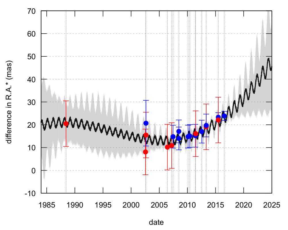 Figure 1
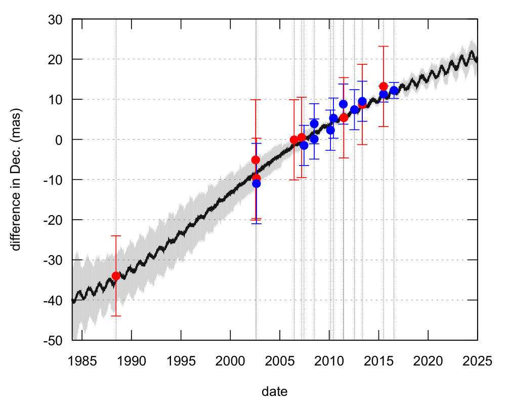 Figure 2
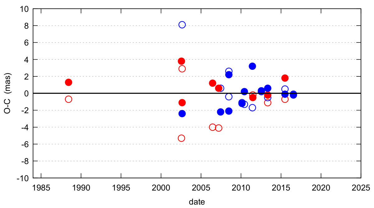 Figure 3
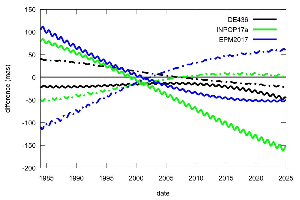 Figure 4
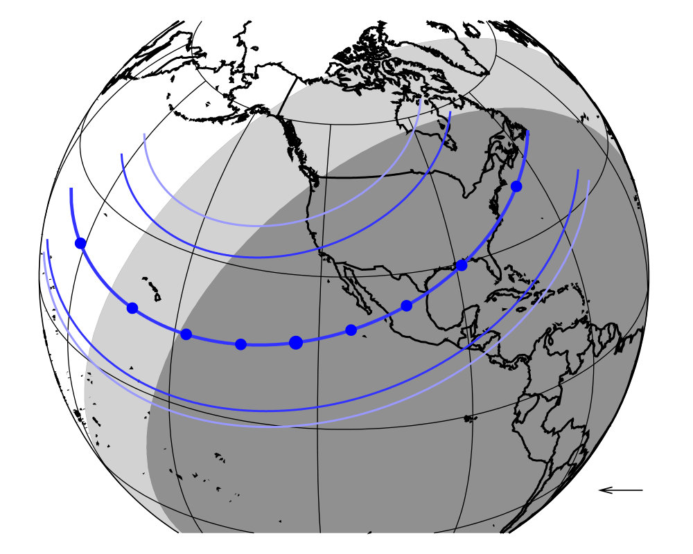 Figure 5
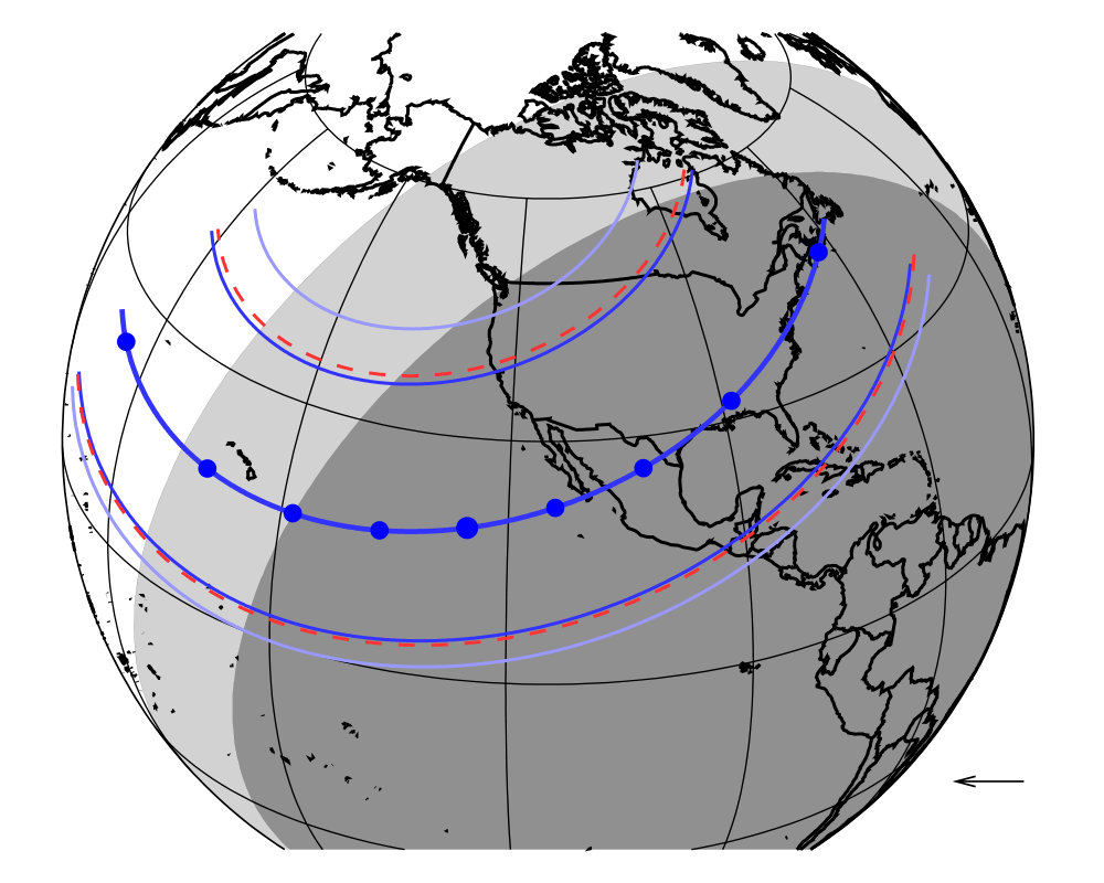 Figure 6
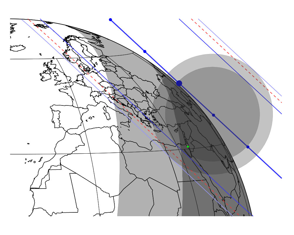 Figure 7
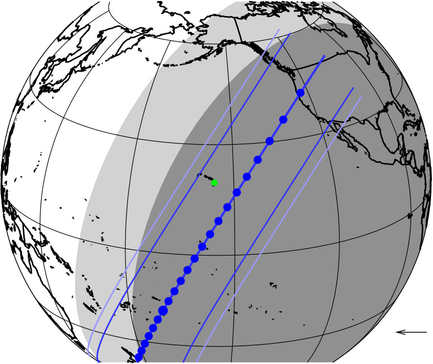 Figure 8
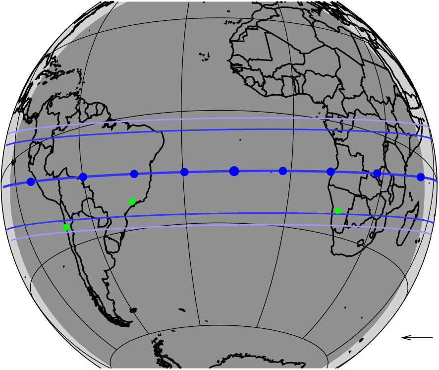 Figure 9
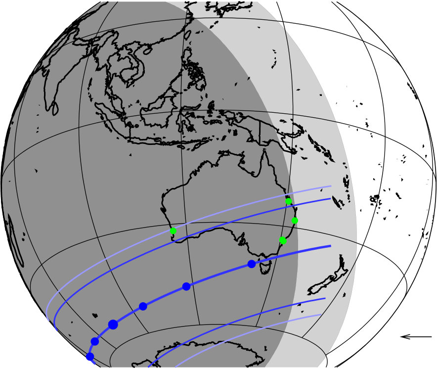 Figure 10
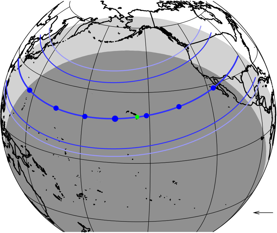 Figure 11
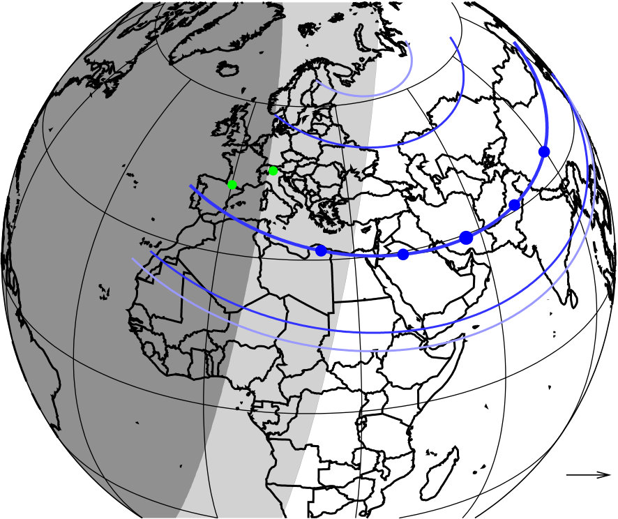 Figure 12
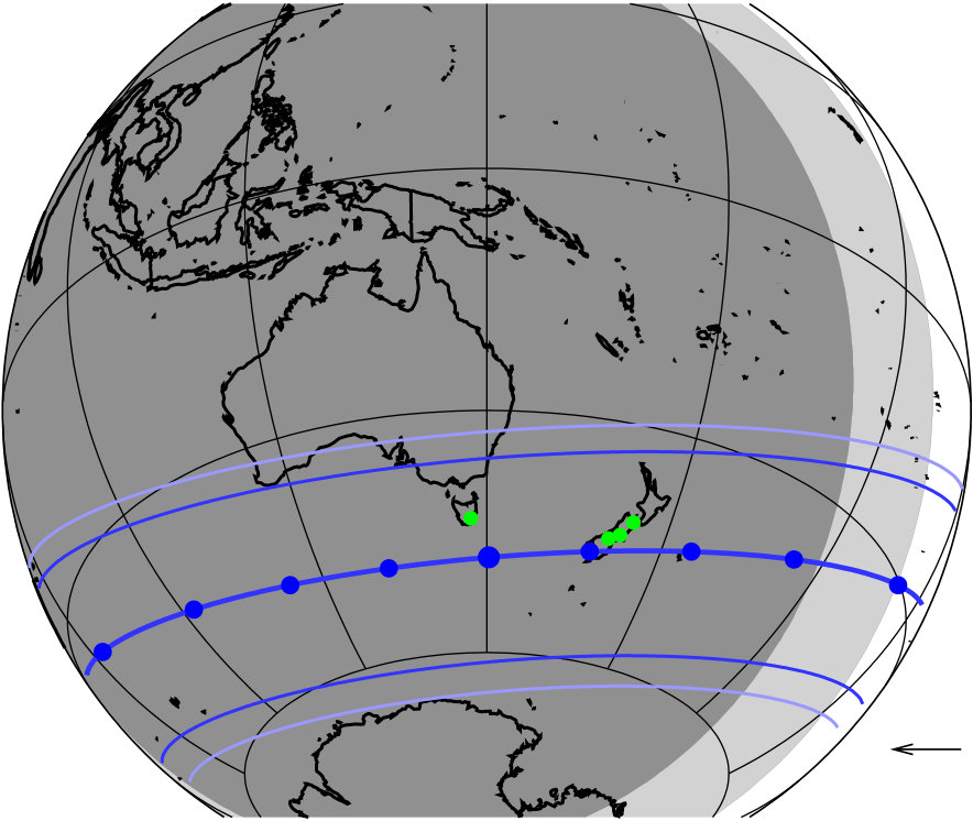 Figure 13
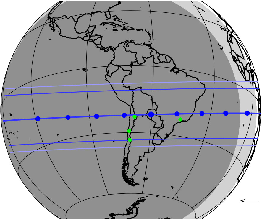 Figure 14
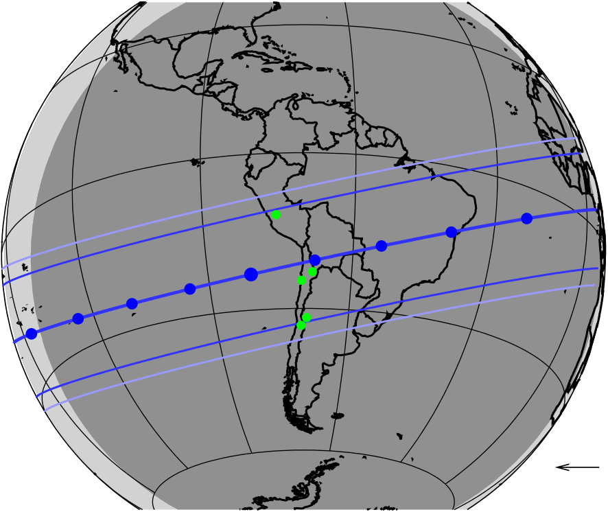 Figure 15
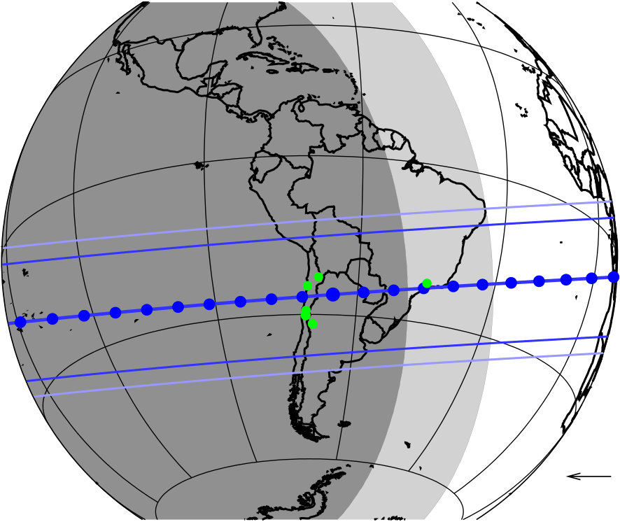 Figure 16
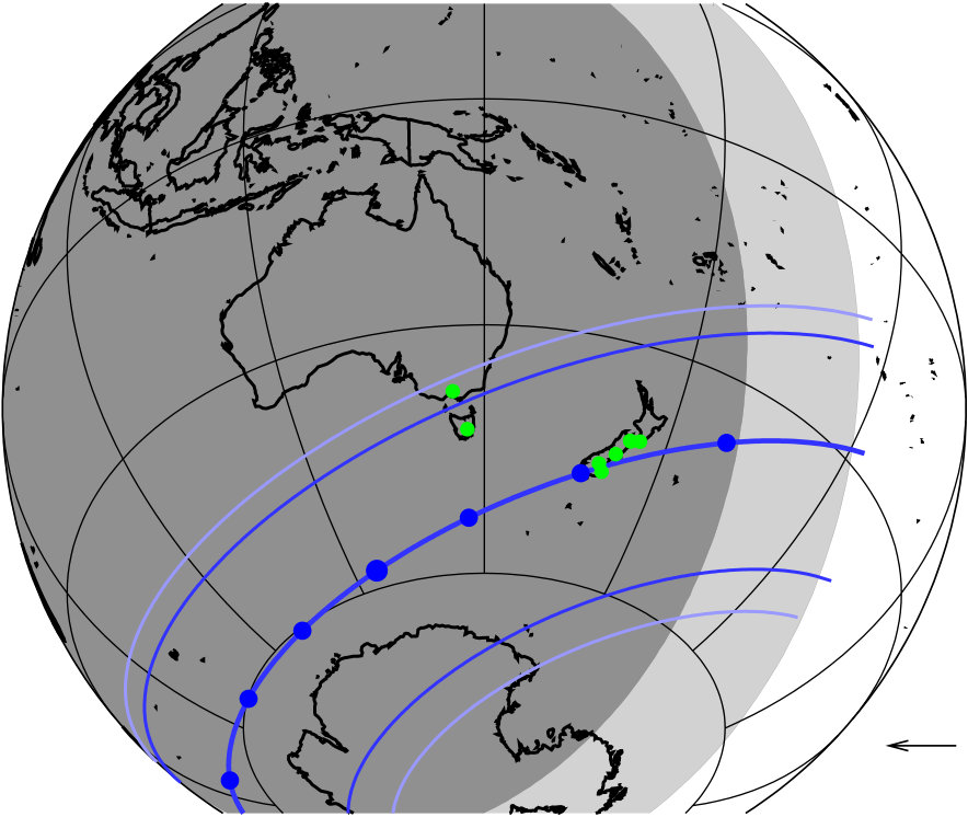 Figure 17
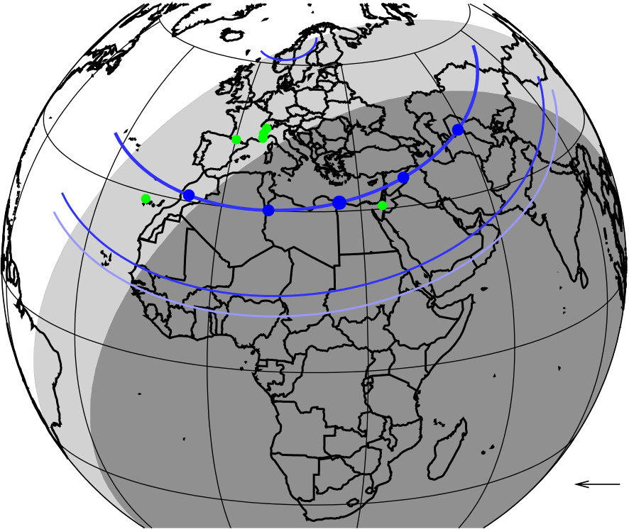 Figure 18
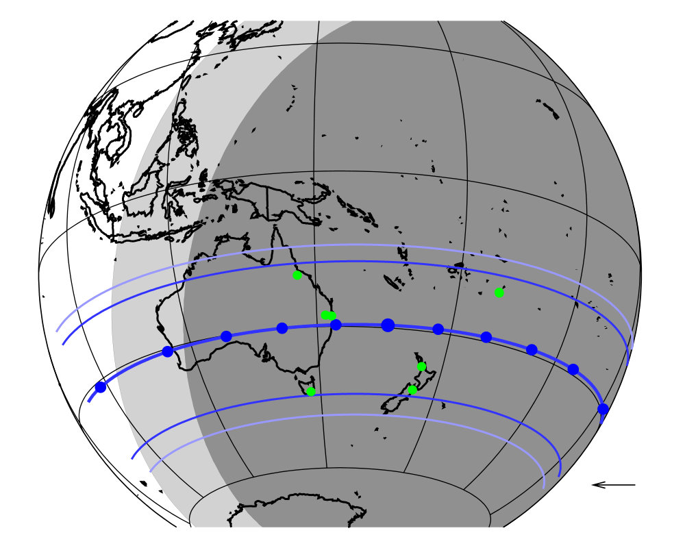 Figure 19
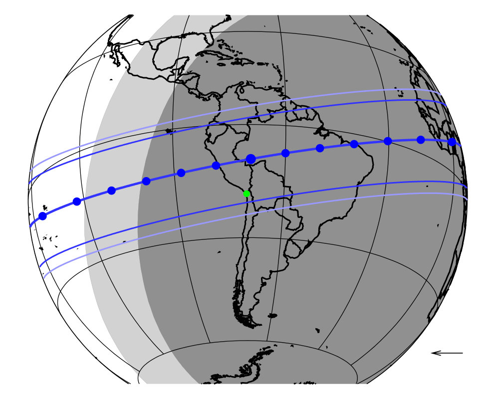 Figure 20
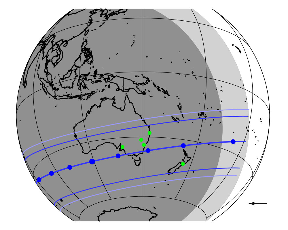 Figure 21
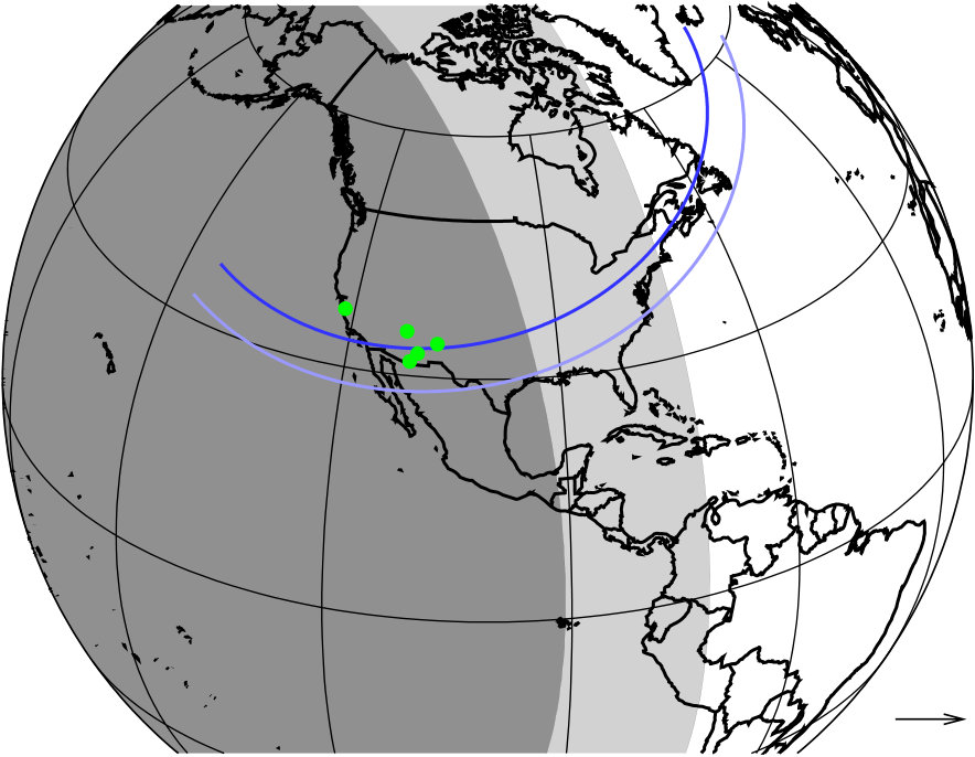 Figure 22
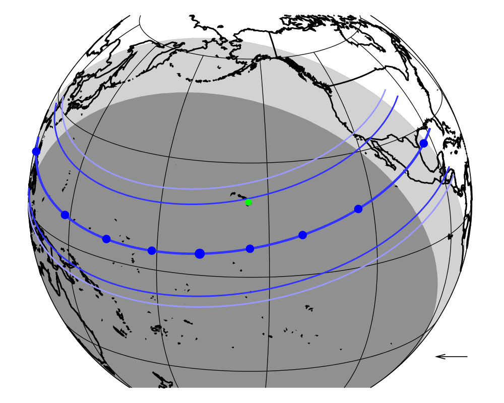 Figure 23
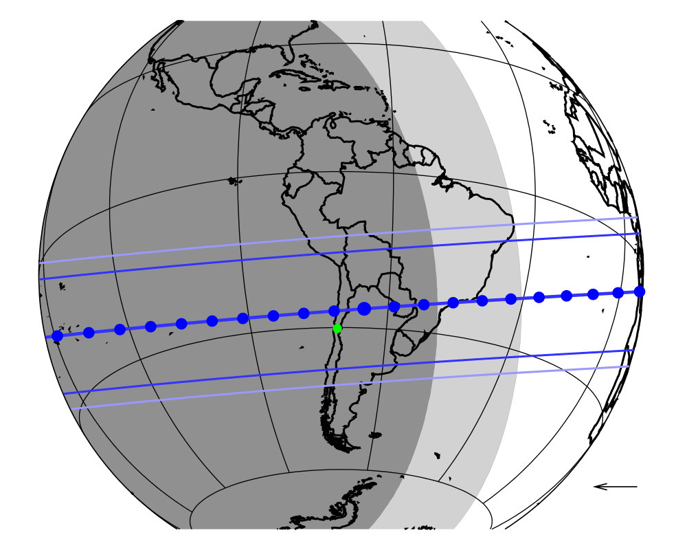 Figure 24
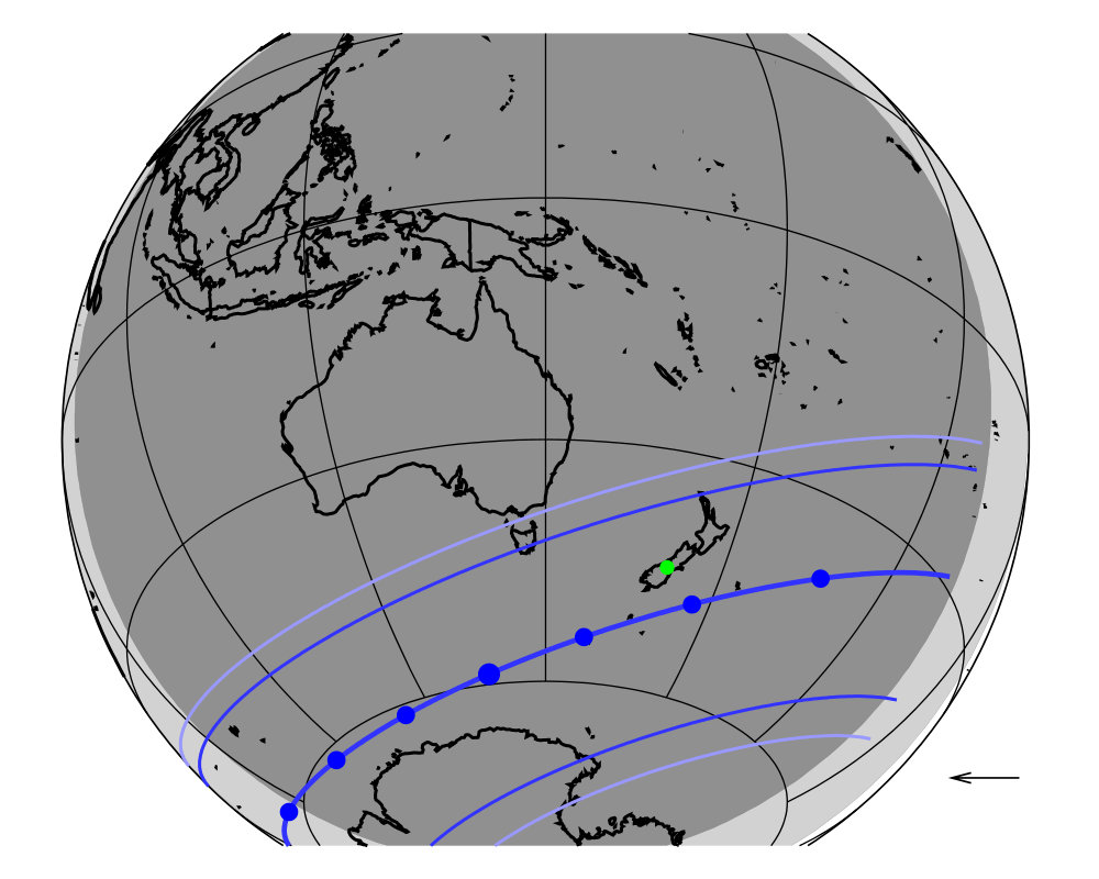 Figure 25
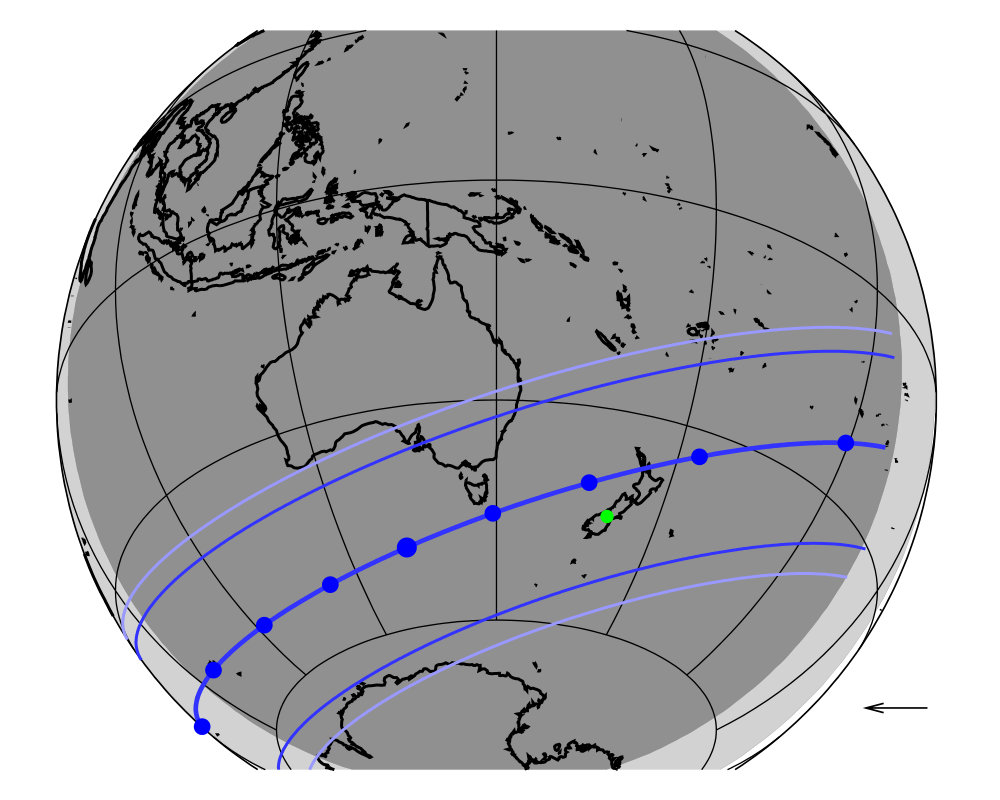 Figure 26
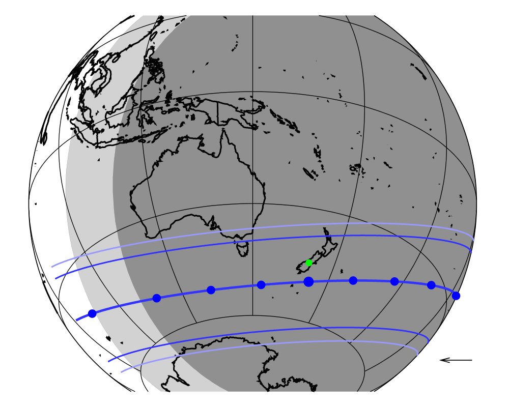 Figure 27
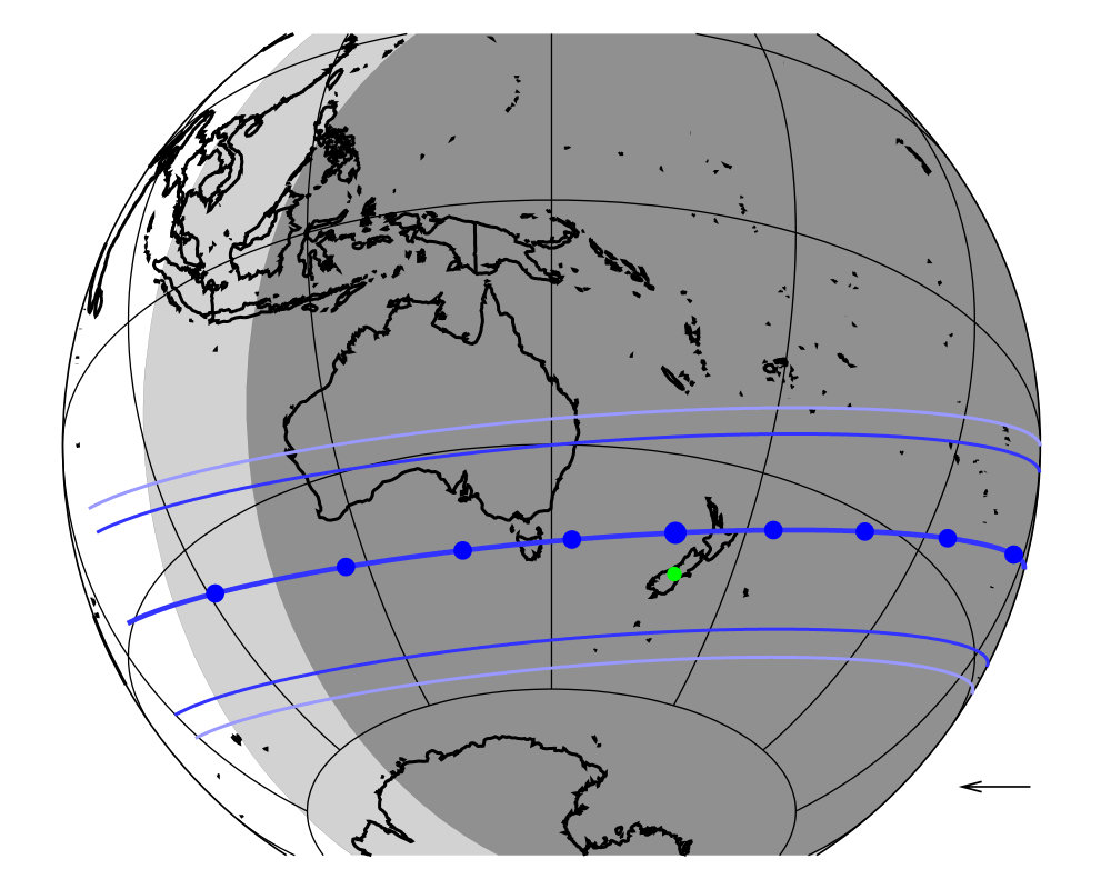 Figure 28
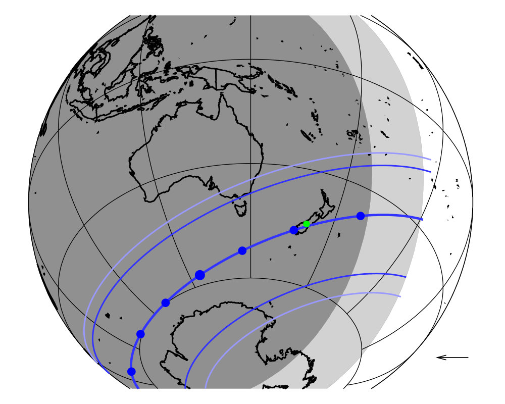 Figure 29
| Reference date | Pluto’s centre position | position of star | ||||
|---|---|---|---|---|---|---|
| right ascension | declination | right ascension | declination | |||
| (mas) | (mas) | |||||
| 2002-08-21 07:00:32 | 16h58m49.4393s | 0.2 | -12∘51’31.944” | 0.1 | 16h58m49.4360s | -12∘51’31.920” |
| 2007-06-14 01:27:00 | 17h50m20.7368s | 0.1 | -16∘22’42.210” | 0.2 | 17h50m20.7392s | -16∘22’42.210” |
| 2008-06-22 19:07:28 | 17h58m33.0303s | 0.2 | -17∘02’38.504” | 0.2 | 17h58m33.0138s | -17∘02’38.349” |
| 2008-06-24 10:37:00 | 17h58m22.3959s | 0.1 | -17∘02’49.177” | 0.7 | 17h58m22.3930s | -17∘02’49.349” |
| 2010-02-14 04:45:00 | 18h19m14.3681s | 0.2 | -18∘16’42.125” | 0.5 | 18h19m14.3851s | -18∘16’42.313” |
| 2010-06-04 15:34:00 | 18h18m47.9476s | 0.3 | -18∘12’51.922” | 1.3 | 18h18m47.9349s | -18∘12’51.794” |
| 2011-06-04 05:42:00 | 18h27m53.8235s | 0.3 | -18∘45’30.741” | 0.3 | 18h27m53.8249s | -18∘45’30.725” |
| 2012-07-18 04:13:00 | 18h32m14.6748s | 0.1 | -19∘24’19.307” | 0.1 | 18h32m14.6720s | -19∘24’19.295” |
| 2013-05-04 08:22:00 | 18h47m52.5333s | 0.1 | -19∘41’24.403” | 0.1 | 18h47m52.5322s | -19∘41’24.374” |
| 2015-06-29 16:02:00 | 19h00m49.7122s | 0.1 | -20∘41’40.399” | 0.1 | 19h00m49.4796s | -20∘41’40.778” |
| 2016-07-19 20:53:45 | 19h07m22.1164s | 0.1 | -21∘10’28.242” | 0.4 | 19h07m22.1242s | -21∘10’28.445” |
| Date | Gaia source identifier | right ascension | declination | Gmag | ||
|---|---|---|---|---|---|---|
| 1988-06-09 | 3652000074629749376 | 14h52m09.962000s | +00∘45’03.30297” | 2.14 | 2.06 | 12.1 |
| 2002-07-20 | 4333071455580364160 | 17h00m18.029957s | -12∘41’42.01220” | 1.12 | 0.73 | 12.6 |
| 2002-08-21 | 4333042833914281856 | 16h58m49.431538s | -12∘51’31.85910” | 1.87 | 1.12 | 15.4 |
| 2006-06-12 | 4124931567980280832 | 17h41m12.074271s | -15∘41’34.47421” | 0.63 | 0.49 | 14.7 |
| 2007-03-18 | 4144912550502784384 | 17h55m05.699098s | -16∘28’34.36682” | 0.74 | 0.60 | 14.8 |
| 2007-06-14 | 4147858103406546048 | 17h50m20.744804s | -16∘22’42.22719” | 0.83 | 0.73 | 15.3 |
| 2008-06-22 | 4144621347334603520 | 17h58m33.013236s | -17∘02’38.39643” | 0.67 | 0.54 | 12.3 |
| 2008-06-24 | 4144621244254585728 | 17h58m22.390423s | -17∘02’49.36558” | 0.93 | 0.78 | 15.6 |
| 2010-02-14 | 4096385295578625536 | 18h19m14.378482s | -18∘16’42.35590” | 0.50 | 0.42 | 10.3 |
| 2010-06-04 | 4096389556186605568 | 18h18m47.930034s | -18∘12’51.82967” | 0.37 | 0.31 | 14.8 |
| 2011-06-04 | 4093175335706340480 | 18h27m53.819996s | -18∘45’30.78871” | 0.62 | 0.50 | 16.4 |
| 2011-06-23 | 4093163211131448704 | 18h25m55.479351s | -18∘48’07.09094” | 0.35 | 0.31 | 14.0 |
| 2012-07-18 | 4092849712861519360 | 18h32m14.673688s | -19∘24’19.34329” | 0.19 | 0.17 | 14.4 |
| 2013-05-04 | 4086200313156846336 | 18h47m52.531982s | -19∘41’24.39714” | 0.10 | 0.09 | 14.2 |
| 2014-07-23 | 4085914882468876672 | 18h49m31.736687s | -20∘22’23.82473” | 0.21 | 0.19 | 17.2 |
| 2014-07-24 | 4085914745029913216 | 18h49m26.511650s | -20∘22’36.98627” | 0.39 | 0.35 | 18.1 |
| 2015-06-29 | 4084956039611370112 | 19h00m49.474124s | -20∘41’40.81016” | 0.04 | 0.04 | 12.0 |
| 2016-07-19 | 4082062610353732096 | 19h07m22.117772s | -21∘10’28.43508” | 0.05 | 0.05 | 13.9 |
| Pluto’s coordinates | O-C (mas) | PLU-BAR (mas) | ||||||
|---|---|---|---|---|---|---|---|---|
| date (UTC) | right ascension | declination | flag | reference | ||||
| 1988-06-09 10:39:17.0 | 14h52m09.96347s | +00∘45’03.1506” | 19.9 | -33.5 | -8.8 | 79.6 | * | Millis et al. (1993) |
| 2002-07-20 01:43:39.8 | 17h00m18.03018s | -12∘41’41.9934” | 7.7 | -4.4 | -52.9 | 24.7 | * | Sicardy et al. (2003) |
| 2002-08-21 07:00:32.0 | 16h58m49.43477s | -12∘51’31.8833” | 20.6 | -10.4 | -51.2 | 48.8 | * | This paper |
| 2002-08-21 07:00:32.0 | 16h58m49.43442s | -12∘51’31.8820” | 15.4 | -9.1 | -51.2 | 48.8 | * | Elliot et al. (2003) |
| 2006-06-12 16:25:05.7 | 17h41m12.07511s | -15∘41’34.5896” | 9.8 | -0.4 | -47.0 | -40.8 | * | Young et al. (2008) |
| 2007-03-18 10:59:33.1 | 17h55m05.69430s | -16∘28’34.0886” | 10.7 | 0.8 | 67.1 | -39.4 | * | Person et al. (2008) |
| 2007-06-14 01:27:00.0 | 17h50m20.74243s | -16∘22’42.2275” | 14.7 | -1.8 | -5.2 | 89.8 | * | This paper |
| 2008-06-22 19:07:28.0 | 17h58m33.02976s | -17∘02’38.5534” | 14.0 | 0.0 | -59.3 | -23.3 | * | This paper |
| 2008-06-24 10:37:00.0 | 17h58m22.39339s | -17∘02’49.1932” | 17.6 | 8.1 | -35.4 | 89.6 | * | This paper |
| 2010-02-14 04:45:00.0 | 18h19m14.36152s | -18∘16’42.1678” | 15.2 | 3.1 | -65.4 | 55.6 | * | This paper |
| 2010-06-04 15:34:00.0 | 18h18m47.94272s | -18∘12’51.9579” | 14.9 | 4.8 | 47.9 | 49.2 | * | This paper |
| 2011-06-04 05:42:00.0 | 18h27m53.81859s | -18∘45’30.8046” | 15.6 | 9.3 | 71.7 | 7.1 | * | This paper |
| 2011-06-23 11:23:48.2 | 18h25m55.47963s | -18∘48’06.9712” | 16.1 | 5.5 | 73.2 | 0.2 | * | Gulbis et al. (2015) |
| 2012-07-18 04:13:00.0 | 18h32m14.67647s | -19∘24’19.3554” | 16.9 | 7.7 | 55.2 | -76.0 | * | This paper |
| 2013-05-04 08:21:41.8 | 18h47m52.53356s | -19∘41’24.4265” | 18.7 | 8.4 | -74.6 | 47.9 | * | Olkin et al. (2015) |
| 2013-05-04 08:22:00.0 | 18h47m52.53305s | -19∘41’24.4265” | 19.3 | 9.2 | -74.6 | 48.0 | * | This paper |
| 2014-07-23 14:25:59.1 | 18h49m31.74100s | -20∘22’23.9915” | 30.4 | 3.7 | -7.5 | -79.7 | Pasachoff et al. (2016) | |
| 2014-07-23 14:25:59.1 | 18h49m31.74048s | -20∘22’23.9502” | 23.0 | 44.9 | -7.5 | -79.7 | Pasachoff et al. (2016) | |
| 2014-07-24 11:42:20.0 | 18h49m26.51393s | -20∘22’37.1172” | 11.3 | -14.6 | -65.8 | -28.7 | Pasachoff et al. (2016) | |
| 2014-07-24 11:42:20.0 | 18h49m26.51337s | -20∘22’37.0734” | 3.4 | 29.1 | -65.8 | -28.7 | Pasachoff et al. (2016) | |
| 2015-06-29 16:02:00.0 | 19h00m49.70680s | -20∘41’40.4308” | 22.8 | 10.7 | -41.9 | 80.3 | * | This paper |
| 2015-06-29 16:54:41.4 | 19h00m49.47778s | -20∘41’40.9707” | 22.1 | 12.7 | -39.4 | 81.2 | * | Pasachoff et al. (2017) |
| 2016-07-19 20:53:45.0 | 19h07m22.10999s | -21∘10’28.2320” | 24.1 | 11.6 | 56.5 | -71.7 | * | This paper |
| date | ||||
|---|---|---|---|---|
| (UTC) | (mas) | (mas) | (mas) | (mas) |
| 1988-06-09 | -0.7 | 1.3 | 10.0 | 10.0 |
| 2002-07-20 | -5.3 | 3.8 | 10.0 | 15.0 |
| 2002-08-21111111Taken from Elliot et al. (2003). | 2.9 | -1.1 | 10.0 | 10.0 |
| 2002-08-21 | 8.1 | -2.4 | 10.0 | 10.0 |
| 2006-06-12 | -4.0 | 1.2 | 10.0 | 10.0 |
| 2007-03-18 | -4.1 | 0.6 | 10.0 | 10.0 |
| 2007-06-14 | 0.6 | -2.2 | 5.0 | 5.0 |
| 2008-06-22 | -0.4 | -2.1 | 5.0 | 5.0 |
| 2008-06-24 | 2.6 | 2.2 | 5.0 | 5.0 |
| 2010-02-14 | -1.1 | -1.2 | 5.0 | 5.0 |
| 2010-06-04 | -1.3 | 0.2 | 5.0 | 5.0 |
| 2011-06-04 | -1.7 | 3.2 | 5.0 | 5.0 |
| 2011-06-23 | -0.2 | -0.5 | 10.0 | 10.0 |
| 2012-07-18 | 0.2 | 0.3 | 5.0 | 5.0 |
| 2013-05-04222222Taken from Olkin et al. (2015). | -1.1 | -0.2 | 10.0 | 10.0 |
| 2013-05-04 | -0.5 | 0.6 | 5.0 | 5.0 |
| 2015-06-29 | 0.5 | -0.1 | 2.0 | 2.0 |
| 2015-06-29333333Taken from Pasachoff et al. (2017). | -0.7 | 1.8 | 10.0 | 10.0 |
| 2016-07-19 | -0.1 | -0.2 | 2.0 | 2.0 |
| observatory | mid-time | ||||
|---|---|---|---|---|---|
| (UTC) | (km) | (s) | (mas) | (mas) | |
| Charters Towers | 10:41:27.1 | 985 | 130.0 | 20.6 | -33.5 |
| Toowoomba | 10:40:50.5 | 188 | 93.4 | 18.4 | -33.6 |
| Mt Tamborine | 10:40:17.4 | 168 | 60.3 | -4.3 | -33.9 |
| Auckland | 10:39:03.3111111Uncertainty of timing in Auckland is not provided in Millis et al. (1993). | -687 | -13.8 | 26.6 | -33.9 |
| Hobart | 10:41:00.6 | -1153 | 103.5 | 19.5 | -33.8 |
| KAO | 10:37:26.9 | 868 | -110.2 | 19.5 | -33.0 |
| Mt John | 10:39:19.6 | -1281 | 2.5 | 19.9 | -33.6 |
| 1988-06-09 10:39:17.1 | 0.006535856 | -0.390599080 | -242.990271254 | -4.176391160 | -47.003163462 | 223.041508925 | 0.750884462 |
|---|---|---|---|---|---|---|---|
| 2002-07-20 01:43:39.8 | -0.015137748 | 0.078729716 | -221.595155776 | -42.613814665 | 45.303191676 | 255.075123563 | -12.694996935 |
| 2002-08-21 07:00:32.0 | 0.091629552 | -0.047418125 | -41.470159949 | -80.186411178 | -27.314474978 | 254.705972362 | -12.858853587 |
| 2006-06-12 16:25:05.8 | 0.008081468 | -0.393907343 | -320.357408358 | -6.588025106 | 39.386450596 | 265.300310118 | -15.692941450 |
| 2007-03-18 10:59:33.1 | -0.283497691 | 0.985999061 | 92.267892934 | 26.509008184 | -58.153737570 | 268.773723165 | -16.476135950 |
| 2011-06-23 11:23:48.2 | -0.043316318 | 0.403059932 | -320.782100593 | -34.487845936 | 50.562763031 | 276.481160400 | -18.801937982 |
| 2013-05-04 08:21:41.8 | 0.013860759 | -0.136954904 | -137.646799082 | -13.969616086 | 16.003277103 | 281.968884350 | -19.690120815 |
| 2014-07-23 14:25:59.1 | 0.110372760 | -0.614706119 | -300.130385882 | -53.903828467 | -20.940785660 | 282.382245191 | -20.373331983 |
| 2014-07-24 11:42:19.9 | 0.075661748 | -0.419500350 | -297.988040527 | -53.754831391 | -22.209299195 | 282.360471376 | -20.376972931 |
| 2015-06-29 16:54:41.4 | 0.106938572 | -0.628240925 | -318.341422110 | -54.232339089 | -2.294494383 | 285.206150857 | -20.694717628 |
Peer Reviews
No public reviews on file for this paper yet. If you reviewed it on a platform where reviews are public (OpenReview, ICLR, NeurIPS, ICML), you can paste yours below so the community can read it here.
Videos
No videos yet. Explain this paper in a talk, walkthrough, or lecture? Add one.
11institutetext: LESIA, Observatoire de Paris, Université PSL, CNRS, Sorbonne Université, Univ. Paris Diderot, Sorbonne Paris Cité, 5 place Jules Janssen, 92195 Meudon, France
11email: [email protected] 22institutetext: Observatório do Valongo/UFRJ, Ladeira Pedro Antonio 43, Rio de Janeiro, RJ 20080-090, Brazil 33institutetext: Observatório Nacional/MCTIC, Laboratório Interinstitucional de e-Astronomia-LIneA and INCT do e-Universo, Rua General José Cristino 77, Rio de Janeiro CEP 20921-400, Brazil 44institutetext: Federal University of Technology - Paraná (UTFPR/DAFIS), Rua Sete de Setembro 3165, CEP 80230-901 Curitiba, Brazil 55institutetext: Escola SESC de Ensino Médio, Avenida Ayrton Senna, 5677, Rio de Janeiro - RJ, 22775-004, Brazil 66institutetext: UNESP - São Paulo State University, Grupo de Dinâmica Orbital e Planetologia, CEP 12516-410, Guaratinguetá, SP 12516-410, Brazil 77institutetext: Geneva Observatory, 1290 Sauverny, Switzerland 88institutetext: Instituto de Astrofísica de Andalucía (IAA-CSIC). Glorieta de la Astronomía s/n. 18008-Granada, Spain
Pluto’s ephemeris from ground-based stellar occultations (1988-2016)
J. Desmars 11
E. Meza 11
B. Sicardy 11
M. Assafin 22
J. I. B. Camargo 33
F. Braga-Ribas 443311
G. Benedetti-Rossi 33
A. Dias-Oliveira 5533
B. Morgado 33
A. R. Gomes-Júnior 6622
R. Vieira-Martins 33
R. Behrend 77
J. L. Ortiz 88
R. Duffard 88
N. Morales 88
P. Santos Sanz 88
(Received December 21, 2018; accepted March 08, 2019)
Abstract
*Context. *From 1988 to 2016, several stellar occultations have been observed to characterize Pluto’s atmosphere and its evolution (Meza et al., 2019). From each stellar occultation, an accurate astrometric position of Pluto at the observation epoch is derived. These positions mainly depend on the position of the occulted star and the precision of the timing.
*Aims. *We present Pluto’s astrometric positions derived from 19 occultations from 1988 to 2016 (11 from Meza et al. (2019) and 8 from other publications). Using Gaia DR2 for the positions of the occulted stars, the accuracy of these positions is estimated to 2-10 milliarcsec depending on the observation circumstances. From these astrometric positions, we derive an updated ephemeris of Pluto’s system barycentre using the NIMA code (Desmars et al., 2015).
*Methods. *The astrometric positions are derived by fitting the occultation’s light curves by a model of Pluto’s atmosphere. The fits provide the observed position of the body’s centre for a reference star position. Other publications usually provide circumstances of the occultation such as the coordinates of the stations, the timing, and the impact parameter (i.e. the closest distance between the station and the centre of the shadow). From these parameters, we use a procedure based on the Bessel method to derive an astrometric position.
*Results. *We derive accurate Pluto’s astrometric positions from 1988 to 2016. These positions are used to refine the orbit of Pluto’system barycentre providing an ephemeris, accurate to the milliarcsec level, over the period 2000-2020, allowing better predictions for future stellar occultations.
Key Words.:
**Astrometry – Celestial mechanics – Ephemerides – Occultations – Kuiper belt objects: individual: Pluto **
1 Introduction
Stellar occultation is a unique technique to obtain the physical parameters of distant objects or to probe their atmosphere and surroundings. For instance, Meza et al. (2019) have used 11 stellar occultations by Pluto from 2002 to 2016 to study the evolution of Pluto’s atmosphere. Meanwhile, occultations allow an accurate determination of the relative position of the body’s centre compared to the position of the occulted star, leading to an accurate astrometric position of Pluto at the time of occultation if the star position is also known accurately.
The accuracy of the body’s position mainly depends on the knowledge of the shape and the size of the body, the modelling of the atmosphere, the precision of the timing system, the velocity of the occultation, the exposure time of the camera, the precision of the stellar position, and the magnitude of the occulted star. Since the publication of the Gaia catalogues in September 2016 for the first release (Gaia Collaboration et al., 2016) and moreover with the second release in April 2018 (Gaia Collaboration et al., 2018) including proper motions and trigonometric parallaxes of the stars, the precision of the stellar catalogues can now reach a tenth of a milliarcsec (mas). For comparison, before Gaia catalogues, the precision of stellar catalogues such as UCAC2 (Zacharias et al., 2004) or UCAC4 (Zacharias et al., 2013), was about 50 to 100 mas per star with also zonal errors. With Gaia, the precision of positions deduced from occultations is expected to be around few mas, taking into account the systematic errors. Thanks to the accuracy of the GaiaDR2 catalogue, occultations can provide the most accurate astrometric measurement of a body in the outer solar system.
In this paper, we present the astrometric positions we derived from occultations presented in Meza et al. (2019) (Sect. 2.1) and in other publications (Sect. 2.2). We detail a method to derive astrometric positions from other publications, knowing the circumstances of occultations: timing and impact parameter (Appendix). Finally, we present in Section 3 a refined ephemeris of Pluto’s system barycentre and we discuss the improvement in the predictions of future occultations by Pluto at a mas level accuracy and as well as the geometry of past events (Sect. 4).
2 Astrometric positions from occultations
2.1 Astrometric positions from occultations in Meza et al. (2019)
Meza et al. (2019) provide 11 occultations by Pluto from 2002 to 2016. Beyond the parameters related to Pluto’s atmosphere, another product of the occultations is the astrometric position of the body. From the geometry of the event, we determine the position of the Pluto’s centre of figure . This position corresponds to the observed position of the object at the time of the occultation for a given star position . In particular, the position of the body we derive, only depends on the star position. Before Gaia catalogues, we determined the star position with our own astrometry. Table 1 gives the position of Pluto’s centre and its precision we derived from the geometry of the occultation and the corresponding star position from our astrometry. With Gaia, the astrometric position of Pluto’s centre can be refined by correcting the star position with the Gaia DR2 star position with the relations:
[TABLE]
This refined position only depends on the Gaia DR2 position which is much more accurate than previous catalogues or our own astrometry. The associated position of the occulted stars in Gaia DR2 catalogue () are listed in Table 1. The positions take into account the proper motions and the parallax from Gaia DR2. The table also presents the Gaia source identifier and the estimated precision of the star position in right ascension and declination, at the time of the occultation, taking into account precision of the stellar position and the proper motions as given in GaiaDR2, for all the occultations studied in this paper.
Finally, Table 3 provides the absolute position in right ascension and declination of Pluto’s centre derived from the geometry and from stellar positions of Gaia DR2. The residuals related to JPL ephemeris222DE436 is a planetary ephemerides from JPL providing the positions of the barycentre of the planets, including the barycentre of Pluto’s system. It is based on DE430 (Folkner et al., 2014). PLU055 is the JPL ephemeris providing the positions of Pluto and its satellites related to the Pluto’s system barycentre, developed by R.Jacobson in 2015 and based on an updated ephemeris of Brozović et al. (2015): https://naif.jpl.nasa.gov/pub/naif/generic_kernels/spk/satellites/plu055.cmt DE436/PLU055 are also indicated as well as the differential positions between Pluto and Pluto’s system barycentre used to refine the orbit (see Sect. 3). A flag indicates if the position is used in the NIMAv8 ephemeris determination. Finally, the reconstructed paths of the occultations are presented in Fig. 7.
2.2 Astrometric positions from other publications
Several authors have published circumstances of an occultation by Pluto (e.g. Millis et al., 1993; Sicardy et al., 2003; Elliot et al., 2003; Young et al., 2008; Person et al., 2008; Gulbis et al., 2015; Olkin et al., 2015; Pasachoff et al., 2016, 2017). From these circumstances (coordinates of the observer, mid-time of the occultation and impact parameter), it is possible to derive an offset between the observation deduced from these circumstances and a reference ephemeris. The procedure, based on the Bessel method used to predict stellar occultations, is described in Appendix A and the details of computation for each occultation are presented in Appendix B. The Pluto’s positions deduced from occultations published in other articles besides those of Meza et al. (2019) are presented in Table 3.
The positions derived from Pasachoff et al. (2016) involving single chord events and faint occulted stars, are not accurate enough to discriminate North and South solutions, i.e. to decide if Pluto’s centre as seen from the observing site passed North or South of the star. Finally, these positions were not used in the orbit determination.
3 NIMA ephemeris of Pluto
NIMA (Numerical Integration of the Motion of an Asteroid) has been developed in order to refine the orbits of small bodies, in particular TNOs and Centaurs studied by stellar occultations technique (Desmars et al., 2015). It consists of the numerical integration of the equations of motion perturbed by gravitational accelerations of the planets (Mercury to Neptune). The Earth and Moon are considered at their barycentre and the masses and the positions of the planets are from JPL DE436.
The use of other masses and positions for planetary ephemeris produces insignificant changes, for example, the difference between the solution using DE436 and the solution using INPOP17a (Viswanathan et al., 2017) for Pluto, is less than 0.06 mas on the 1985-2025 period. Moreover, there is no need to take into account the gravitational perturbations of the biggest TNOs. For example, by adding the 6 biggest TNOs (Eris, Haumea, 2007 OR10, Makemake, Quaoar and Sedna) in the model, the difference between the solutions with and without the biggest TNOs are about 0.04 mas in right ascension and declination on the 1985-2025 period, which is 100 times smaller than the mas-level accuracy of the astrometric positions.
The state vector (the heliocentric vector of position and velocity of the body at a specific epoch) is refined by fitting to astrometric observations with the least square method. The main advantage of NIMA is allowing for the use of observations published on the Minor Planet Center444The Minor Planet Center is in charge of providing astrometric measurements, orbital elements of the solar system small bodies : http://minorplanetcenter.net. together with unpublished observations or astrometric positions of occultations. The quality of the observations is taken into account with a specific weighting scheme, in particular, it takes advantages of the high accuracy of occultations. Finally, after fitting to the observations, NIMA can provide an ephemeris through a bsp file format readable by the SPICE library555The SPICE Toolkit is a library developed by NASA dedicated to space navigation and providing in particular a list of routines related to ephemeris: http://naif.jpl.nasa.gov/naif/index.html..
As NIMA is representing the motion of the centre of mass of an object, it allows to compute the position of the Pluto’s system barycentre and not the position of Pluto’s centre itself. To deal with positions derived from occultations, we need an additional ephemeris representing the position of Pluto relative to its system barycentre. For that purpose, we use the most recent ephemeris PLU055 developed in 2015. The occultation-derived positions are then corrected from the offset between Pluto and the Pluto’s system barycentre (see Table 3) to derive the barycentric positions from the occultations, then used in the NIMA fitting procedure.
The precisions of the positions in right ascension and in declination derived from the occultations are provided in Table 1 for occultations presented in Meza et al. (2019) and in Appendix B for other publications. This precision is deduced from a specific model and reduction (for occultations in Meza et al. 2019) and from the precisions of timing and impact parameters (for other publications), without any estimation of systematic errors. For a realistic estimation of the orbit accuracy, the weighting scheme in the orbit fit needs to take into account the systematic errors (see Desmars et al. 2015 for details). The global accuracy for the positions used in the fitting depends on the accuracy of the stellar positions (from 0.1 to 2 mas), the precision of the derived position (from 0.1 mas to 11 mas), and the accuracy of the Pluto body-Pluto system barycentre ephemeris (estimated to 1-5 mas).
The errors on Pluto’s centre determination have in fact various sources: the noise present in each occultation light curve and the spatial distribution of the occultation chords across the body. Assuming a normal noise, a formal error on the centre of the planet can then be derived, using a classical least-square fitting and estimation. However, other systematic errors may also be present, such as problems in the absolute timing registration, slow sky transparency variations that make the photometric noise non-gaussian. Finally, the particular choice of the atmospheric model may also induce systematic biases in the centre determination. All those systematic errors are difficult to trace back. In that context, it is instructive to compare the reconstructions of the geometry of a given occultation by independent groups that used different chords and different Pluto’s atmospheric models. For example, occultations on 21 August 2002, 4 May 2013 and 29 June 2015 (see Table 4) indicate differences of few mas, which is much higher than the respective internal precisions (order of 0.1 mas). Case by case studies should be undertaken to explain those inconsistencies. This remains out of the scope of this paper. Meanwhile, for the weighting scheme in the orbit fit, we adopt the estimated precision presented in Table 4 taking into account an estimation of systematic errors for each occultation.
Figure 1 shows the difference between NIMA666The NIMAv8 ephemeris is available on http://lesia.obspm.fr/lucky-star/nima.php. and JPLDE436 ephemeris of Pluto’s barycentre in right ascension (weighted by ) and declination. The blue bullets and the error bars represent the positions and their estimated precision from our occultations, the red bullets represent the positions from occultations not listed in Meza et al. (2019): Millis et al. (1993); Sicardy et al. (2003); Elliot et al. (2003); Young et al. (2008); Person et al. (2008); Gulbis et al. (2015); Olkin et al. (2015); Pasachoff et al. (2017), and the gray area represents the one sigma uncertainty of the NIMAv8 ephemeris.
Table 4 and Fig. 2 provide the residuals (O-C) of the positions derived from the occultations, compared with the NIMAv8 ephemeris, and the estimated precision of the positions used in the weighting scheme. After 2011, residuals are mostly below the mas level, which is much better than any ground-based astrometric observation of Pluto. In that context, other classical observations of Pluto, such as CCD, appear to be less useful for ephemerides of Pluto during the period covered by the occultations 1988-2016.
Figure 3 shows the difference in right ascension and declination between the most recent ephemerides of Pluto system barycentre: JPL DE436, INPOP17a (Viswanathan et al., 2017) and EPM2017 (Pitjeva & Pitjev, 2014) compared to NIMAv8. These differences are mostly due to data and weights used for the orbit determination. They reveal periodic terms in the orbit of Pluto system barycentre that are differently estimated in orbit determination. As described in Desmars et al. (2015), the one-year period corresponds to the parallax induced by different geocentric distances given by the ephemerides. It is also another good indication of the improvement of the NIMAv8 ephemeris since the differences between these ephemerides reach 50-100 mas whereas the estimated precision of NIMAv8 is 2-20 mas on the same period.
4 Discussion
The NIMA ephemeris allows very accurate predictions of stellar occultation by Pluto in the forthcoming years within a few mas level. In particular, we have predicted an occultation of a magnitude 13 star888The star position in Gaia DR2 at the epoch of the occultation is 19h22m10.4687s in right ascension and in declination. by Pluto on August 15, 2018, above North America to the precision of 2.5 mas, representing only 60 km on the shadow path and a precision of 4 s in time. As shown in Meza et al. (2019), the observation of a central flash allows to probe the deepest layers of Pluto’s atmosphere. The central flash can be observed in an small band about 50 km around the centrality path. By reaching a precision of tens of km, we were able to gather observing stations along the centrality and to highly increase the probability of observing a central flash.
The prediction of the August 15, 2018 Pluto occultation was used to assess the accuracy of our predictions using the NIMA approach. Figure 4 represents the prediction of the occultation by Pluto on August 15, 2018 using two different ephemerides: JPL DE436/PLU055 and NIMAv8/PLU055. The prediction using JPL ephemerides is shifted by 36.8 s and 8 mas south (representing about 190 km) compared to the prediction with NIMAv8 ephemeris. Several stations detected the occultation, some of them revealing a central flash. For instance, observers at George Observatory (Texas, USA) report a central flash of typical amplitude 20%, compared to the unocculted stellar flux (T. Blank and P. Maley, private communications).
As the amplitude of the flash roughly scales as the inverse of the closest approach (C/A) distance of the station to the shadow centre, the amplitude may serve to estimate the C/A distance. A central flash reported by Sicardy et al. (2016) was observed at a station in New Zealand during the June 29, 2015 occultation. It had an amplitude of 13%, with C/A distance of 42 km. Thus, the flash observed at George Observatory provides an estimated C/A distance of 25 km for that station. This agrees with the value predicted by the NIMAv8/PLU055 ephemeris, to within 3 km, corresponding to 0.12 mas. This is fully consistent with, but smaller than our 2.5 mas error bar quoted above, possibly indicating an overestimation of our prediction errors.
The precision of our predictions remains at few mas up to 2025 (in particular in declination) and it is even more important since the apparent position of Pluto as seen from Earth is moving away from the Galactic centre, making occultations by Pluto more rare.
Another point of interest is to look at past occultations. In particular, for the occultation of August 19, 1985, Brosch & Mendelson (1985) reported a single chord occultation of a magnitude 11.1 star999The star position in Gaia DR2 at the epoch of the occultation is 14h23m43.4575s in right ascension and in declination. by Pluto, showing a gradual shape possibly due to Pluto’s atmosphere. The observation was performed at Wise observatory in Israel under poor conditions (low elevation, flares from passing planes, close to twilight). Thanks to Gaia DR2 providing the proper motion of the star and to NIMAv8, we make a postdiction of the occultation of August 19, 1985 (Fig. 5). The nominal time for the occultation (the time of the closest approach between the geocentre and the centre of the shadow) is 17:58:57.1 (UTC) leading to a predicted mid-time of 17:59:49.8 (UTC) at Wise observatory. Brosch (1995) gave an approximate observed mid-time of the occultation for Wise observatory at 17:59:54 (about 4 s later than the prediction). The predicted shadow of Pluto at the same time is presented on the figure as well as the observatory’s place as a green bullet. Taking into account the uncertainties of the NIMAv8 ephemeris and of the star position, the uncertainty in time for this occultation is about 20 s whereas the crosstrack uncertainty on the path is about 10 mas (representing 220 km). This is fully consistent with the fact that the occultation was indeed observed at Wise observatory.
5 Conclusions
Stellar occultations by Pluto provide accurate astrometric positions thanks to Gaia catalogues, in particular Gaia DR2. We determine 18 astrometric positions of Pluto from 1988 to 2016 with an estimated precision of 2 to 10 mas.
These positions are used to compute an ephemeris of Pluto system’s barycentre thanks to NIMA procedure with an unprecedented precision on the 1985-2015 period. This ephemeris NIMAv8 was used to study the possible occultation of Pluto observed in 1985 as well to predict the recent occultation by Pluto on August 15th, 2018 or the forthcoming occultations101010See the predictions on the Lucky Star webpage http://lesia.obspm.fr/lucky-star/predictions.php. with a precision of 2 mas, a result impossible to reach with classical astrometry and previous stellar catalogues. In fact, the presence of the usually unresolved Charon in classical images, causes significant displacements of the photocentre of the system with respect to its barycentre. As a consequence, and even modeling the effect of Charon, as in Benedetti-Rossi et al. (2014), accuracies below the 50 mas level are difficult to reach.
This method can be extended, for instance for Chariklo, with an even better accuracy of the order of 1 mas (Desmars et al., 2017) and illustrates the power of stellar occultations not only for better studying those bodies, but also for improving their orbital elements.
Acknowledgements.
Part of the research leading to these results has received funding from the European Research Council under the European Community’s H2020 (2014–2020/ERC Grant Agreement No. 669416 “LUCKY STAR”). This work has made use of data from the European Space Agency (ESA) mission Gaia (https://www.cosmos.esa.int/gaia), processed by the Gaia Data Processing and Analysis Consortium (DPAC, https://www.cosmos.esa.int/web/gaia/dpac/consortium). Funding for the DPAC has been provided by national institutions, in particular the institutions participating in the Gaia Multilateral Agreement. J.I.B.C. acknowledges CNPq grant 308150/2016-3. M.A. thanks CNPq (Grants 427700/2018-3, 310683/2017-3 and 473002/2013-2) and FAPERJ (Grant E-26/111.488/2013). G.B.R. is thankful for the support of the CAPES (203.173/2016) and FAPERJ/PAPDRJ (E26/200.464/2015-227833) grants. This study was financed in part by the Coordenação de Aperfeiçoamento de Pessoal de Nível Superior - Brasil (CAPES) - Finance Code 001. F.B.R.acknowledges CNPq grant 309578/2017-5. A.R.G-J thanks FAPESP proc. 2018/11239-8. R.V-M thanks grants: CNPq-304544/2017-5, 401903/2016-8, Faperj: PAPDRJ-45/2013 and E-26/203.026/2015 P.S.-S. acknowledges financial support by the European Union’s Horizon 2020 Research and Innovation Programme, under Grant Agreement no 687378, as part of the project ”Small Bodies Near and Far” (SBNAF).
Appendix A Method to derive astrometric positions from occultation’s circumstances
We present in this section a method to derive an astrometric position from an occultation’s observation, knowing the occultation’s circumstances. The determination of an occultation’s circumstances consists in computing the Besselian elements. The Bessel method makes use of the fundamental plane that passes through the centre of the Earth and perpendicular to the line joining the star and the centre of the object (i.e. the axis of the shadow). The method is for example described in Urban & Seidelmann (2013). The Besselian elements are usually given for the time of conjunction of the star and the object in right ascension but in this paper the reference time is the time of closest angular approach between the star and the object.
The Besselian elements are the UTC time of the closest approach, the Greenwich Hour Angle of the star at , and the coordinates of the shadow axis at in the fundamental plane, and the rates of changes in and at , and the right ascension and the declination of the star. Their computation are fully described in Urban & Seidelmann (2013).
The quantities and depend on the ephemeris of the body and allow to represent the linear motion of the shadow at the time of the occultation. In this paper, are expressed in Earth radius unit and are in Earth radius per day.
From and , the coordinates111Latitude refers to geocentric latitude. Usually coordinates provide geodetic latitude that need to be converted to geocentric latitude. of the shadow centre at can be derived.
For an observing site, the method requires the local circumstances which are the mid-time of the occultation and the impact parameter , the distance of closest approach between the site and the centre of the shadow in the fundamental plane. Usually, the impact parameter is given in kilometres and when the occultation has only one chord, two solutions (North and South) can be associated.
The first step is to add a shift to and to take into account the impact parameter, i.e. the fact that the observing site is not right on the centrality of the occultation.
[TABLE]
where is the ratio between and Earth radius.
Given the longitude and the latitude111Latitude refers to geocentric latitude. Usually coordinates provide geodetic latitude that need to be converted to geocentric latitude. of the observing site, the coordinates in the fundamental plane are given by :
[TABLE]
The time of the closest approach for the observer is given by the relation :
[TABLE]
In fact, are calculated iteratively by replacing by , where is the rate of Earth’s rotation, to take into account the Earth’s rotation during .
If is the difference between the observed time of the occultation for the observer and the nominal time of the occultation , the correction to apply to the Besselian elements are :
[TABLE]
The quantities are determined iteratively and finally transformed into an offset in right ascension and in declination between the observed occultation and the predicted occultation (from the ephemeris).
For single chord occultation, there are two solutions (North and South), meaning that we do not know whether Pluto’s center went North or South of the star as seen from the observing site. Conversely, for multi-chord occultation there is a unique solution. In that case, the astrometric position deduced from the occultation is the reference ephemeris plus the average offset deduced from all the observing sites.
This is a powerful method to derive astrometric positions from occultations. It only requires local circumstances of the occultation for the observing sites such as the mid-time of the occultation and the impact parameter. If the impact parameter is not provided, one can deduce it from the timing of immersion and emmersion knowing the size of the object and assuming it is spherical. Thus, the method can be used for any object.
Appendix B Astrometric positions from other occultations
In this section, we derive astrometric positions from occultations published in various articles using the method previously presented. The Besselian elements corresponding to the occultations are presented in Table 5 and the reconstructed shadow trajectories of occultation are presented in Fig. 9.
B.1 Occultation of 9 June 1988
Millis et al. (1993) presented the June 9, 1988 Pluto occultation. They derived an astrometric solution by giving the impact parameter for the eight stations that recorded the event.
According to the mid-time of the occultation derived from the paper, we determine the following offsets:
For Black Birch, there is only the immersion timing so the mid-time of the occultation cannot be derived. The average offset of this occultation was determined using the same set of the preferred astrometric solution of Millis et al. (1993), i.e. data from Charters Towers, Hobart, Kuiper Airbone Observatory (KAO) and Mount John.
Finally, we derive the average offset of mas and mas.
B.2 Occultation of 20 July 2002
Sicardy et al. (2003) obtained a light curve of the occultation by Pluto near Arica, North of Chile. They derived an astrometric solution of the occultation by giving distance of closest approach to the centre of Pluto’s shadow for Arica (km).
In Arica, the mid-time of the occultation occurs at 01:44:03 (UTC), giving s. There are two possible solutions but the occultation was also observed at Mamiña111111The Mamiña coordinates are S and W. in Chile (Buie, personal communication) so the only possible solution is the South one.
Finally, we derive the offset of mas and mas, assuming a precision of 2 s for the mid-time.
B.3 Occultation of 21 August 2002
Elliot et al. (2003) derived an astrometric solution of the occultation by giving distance of closest approach to the centre of Pluto’s shadow for Mauna Kea Observatory (km) and Lick Observatory (km). They observed a positive occultation with three telescopes (two in Hawaii and one at Lick Observatory).
As there are at least two stations observing this occultation, there is a unique solution. According to the mid-time of the occultation in the two stations, we derived the following offsets:
[TABLE]
Finally, for this occultation, we used an average offset of mas and mas.
B.4 Occultation of 12 June 2006
Young et al. (2008) presented the analysis of an occultation by Pluto on 12 June 2006. They published the half light time (ingress and egress) and the impact parameter (closest distance to the centre of the shadow) for five stations:
- •
REE = Reedy Creek Observatory, QLD, AUS (0.5 m aperture).
- •
AAT = Anglo-Australian Observatory, NSW, AUS (4 m).
- •
STO = Stockport Observatory, SA, AUS (0.5 m).
- •
HHT = Hawkesbury Heights, NSW, AUS (0.2 m).
- •
CAR = Carter Observatory, Wellington, NZ (0.6 m)
These parameters allow us to compute the mid-time of the occultation and to finally derive an offset for each station:
[TABLE]
Finally, for this occultation, we used an average offset of mas and mas.
B.5 Occultation of 18 March 2007
Person et al. (2008) presented an analysis of an occultation by Pluto observed in several places in USA on 18 March 2007.
From five stations, they derived the geometry of the event by providing the mid-time (UTC) of the event at 10:53:4900:01 (giving s) and an impact parameter of km for the Multiple Mirror Telescope Observatory (MMTO).
According to the geometry of the event, the South solution ( km) has to be adopted, giving the offset related to JPL DE436/PLU055 ephemeris of mas and mas.
B.6 Occultation of 23 June 2011
Gulbis et al. (2015) presented a grazing occultation by Pluto observed in IRTF (Mauna Kea Observatory) on 23 June 2011. They derived an impact parameter of km and a mid-time (UTC) of the event at 11:23:03.07 ( s).
The single chord leads to two possible solutions providing the following offset related to JPL DE436/PLU055 ephemeris:
[TABLE]
According to Gulbis et al. (2015), the North solution has to be adopted. Finally, the offset is mas and mas, assuming the estimated precision of the timing and the impact parameter.
B.7 Occultation of 04 May 2013
Olkin et al. (2015) presented the occultation by Pluto on 4 May 2013 observed in South America.
They derived the mid-time (UTC) of the event at 08:23:21.60s (giving s) and an impact parameter of km for the LCOGT at Cerro Tololo.
From these circumstances, we derived an offset related to JPL DE436/PLU055 ephemeris of mas and mas
B.8 Occultation of 23 July 2014
Pasachoff et al. (2016) published the observation of two single-chord occultations at Mont John (New Zealand) on June 2014. They provided the timing and impact parameter for the two occultations.
The fitted impact parameter for 23 July is km providing two possible solutions and the mid-time (UTC) of the occultation 14:24:31s is derived from the ingress and egress times at 50% and corresponds to s.
Each solution provides the following offset related to JPL DE436/PLU055 ephemeris:
[TABLE]
According to the precisions of the mid-time and of the impact parameter, the estimated precision of the offset is 4.0 mas for and 5.2 mas for .
B.9 Occultation of 24 July 2014
Pasachoff et al. (2016) also provided circumstances of the occultation on 24 July 2014 at Mont John Observatory.
The fitted impact parameter is km providing two possible solutions and the mid-time (UTC) of the occultation 11:42:29s is derived from the ingress and egress times at 50% and corresponds to s.
Each solution provides the following offset related to JPL DE436/PLU055 ephemeris:
[TABLE]
According to the precisions of the mid-time and of the impact parameter, the estimated precision of the offset is 7.7 mas for and 6.1 mas for .
B.10 Occultation of 29 June 2015
Pasachoff et al. (2017) presented the occultation by Pluto on 29 June 2015.
They derived the mid-time (UTC) of the event at 16:52:50 (giving s) and an impact parameter of km for the Mont John Observatory in New Zealand.
From these circumstances, we derived an offset of mas and mas related to JPL DE436/PLU055 ephemeris. The precision of the offset cannot be determined since the precision in mid-time and in the impact parameter are not indicated.
The reference list from the paper itself. Each links out to its DOI / PubMed record.
- 1Benedetti-Rossi et al. (2014) Benedetti-Rossi, G., Vieira Martins, R., Camargo, J. I. B., Assafin, M., & Braga-Ribas, F. 2014, A&A, 570, A 86
- 2Brosch (1995) Brosch, N. 1995, MNRAS, 276, 571
- 3Brosch & Mendelson (1985) Brosch, N. & Mendelson, H. 1985, IAU Circ., 4097
- 4Brozović et al. (2015) Brozović, M., Showalter, M. R., Jacobson, R. A., & Buie, M. W. 2015, Icarus, 246, 317
- 5Desmars et al. (2017) Desmars, J., Camargo, J., Bérard, D., et al. 2017, in AAS/Division for Planetary Sciences Meeting Abstracts, Vol. 49, AAS/Division for Planetary Sciences Meeting Abstracts #49, 216.03
- 6Desmars et al. (2015) Desmars, J., Camargo, J. I. B., Braga-Ribas, F., et al. 2015, A&A, 584, A 96
- 7Elliot et al. (2003) Elliot, J. L., Ates, A., Babcock, B. A., et al. 2003, Nature, 424, 165
- 8Folkner et al. (2014) Folkner, W., Williams, J., Boggs, D., Park, R., & Kuchynka, P. 2014, JPL IPN Progress Reports, 42-196, http://ipnpr.jpl.nasa.gov/progress_report/42-196/196C.pdf