Reconstruction of $f(R)$ gravity models for an accelerated universe using Raychaudhuri equation
Shibendu Gupta Choudhury, Ananda Dasgupta, Narayan Banerjee

TL;DR
This paper introduces a new method using Raychaudhuri equation to reconstruct $f(R)$ gravity models for accelerated universes, but finds the models are not viable in the tested scenarios.
Contribution
It presents an analytical reconstruction approach for $f(R)$ gravity models based on kinematic universe parameters using Raychaudhuri equation.
Findings
Reconstructed $f(R)$ models for accelerating universe scenarios.
Models involve power-law and hypergeometric functions.
Reconstructed models are found to be non-viable.
Abstract
A new strategy for the reconstruction of gravity models have been attempted using Raychaudhuri equation. Two examples, one for an eternally accelerating universe and the other for one that mimics a CDM expansion history have been worked out. For both the cases, the relevant could be found out analytically. In the first case, is found to be a combination of power-law terms and in the expression for the second case involves hypergeometric functions. The evolution history of the universe, given as specific values of the kinematical quantities like the jerk or the deceleration parameter, serve as the input. It is found that the corresponding gravity models, in both the examples, are not viable options.
Click any figure to enlarge with its caption.
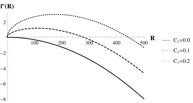 Figure 1
 Figure 2
 Figure 3
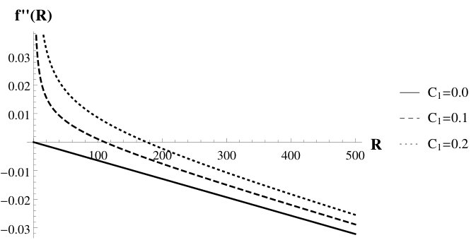 Figure 4
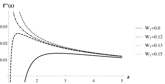 Figure 5
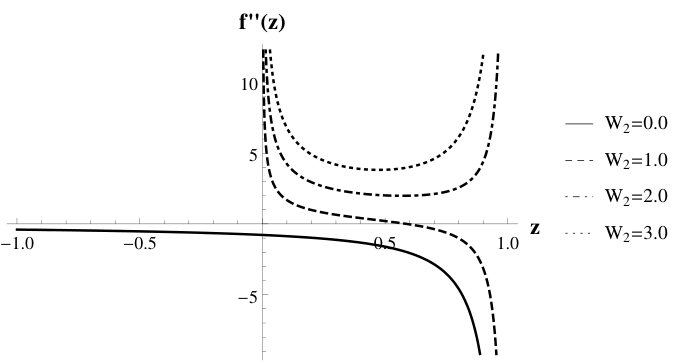 Figure 6
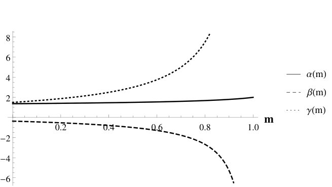 Figure 7
| Singular Point | Solution | Range of applicability |
|---|---|---|
Peer Reviews
No public reviews on file for this paper yet. If you reviewed it on a platform where reviews are public (OpenReview, ICLR, NeurIPS, ICML), you can paste yours below so the community can read it here.
Videos
No videos yet. Explain this paper in a talk, walkthrough, or lecture? Add one.
Reconstruction of gravity models for an accelerated universe using Raychaudhuri equation
Shibendu Gupta Choudhury1, Ananda Dasgupta1, Narayan Banerjee1
1Department Of Physical Sciences, IISER Kolkata, Mohanpur, Nadia 741235, India E-mail: [email protected]: [email protected]: [email protected]
(Accepted ??. Received ??; in original form ??)
Abstract
A new strategy for the reconstruction of gravity models have been attempted using Raychaudhuri equation. Two examples, one for an eternally accelerating universe and the other for one that mimics a CDM expansion history have been worked out. For both the cases, the relevant could be found out analytically. In the first case, is found to be a combination of power-law terms and in the expression for the second case involves hypergeometric functions. The evolution history of the universe, given as specific values of the kinematical quantities like the jerk or the deceleration parameter, serve as the input. It is found that the corresponding gravity models, in both the examples, are not viable options.
keywords:
dark energy, cosmological parameters
††pubyear: ????††pagerange: Reconstruction of gravity models for an accelerated universe using Raychaudhuri equation–References
1 Introduction
Arguably, the most talked about but unresolved puzzle in cosmology for the last twenty years has been that of “Dark Energy”, the driver of the alleged accelerated expansion of the universe (, 2016; Haridasu et al., 2017). Although a non-zero cosmological constant can indeed match the observational data (Padmanabhan, 2003), its observationally required value appears to be too small compared to the theoretically predicted value. Quintessence models, which are scalar fields with a potential, also do very well in explaining the cosmological data with a bit of fine tuning, but there is hardly any strongly motivated scalar field model with support for that from theoretical particle physics. For a recent account of various dark energy models, we refer to the work of Brax (2018).
A parallel approach towards finding a resolution of accelerated expansion is to modify the theory of gravity rather than to introduce an exotic matter. Examples of such attempts include a non-minimally coupled scalar field theory (Bertolami & Martins, 2000; Banerjee & Pavon, 2001) or an theory of gravity (Capozziello et al., 2003; Nojiri & Odintsov, 2003a, b; Carroll et al., 2004; Das, Banerjee & Dadhich, 2006). In an gravity model, the Ricci scalar in the Einstein-Hilbert action is generalised to , an analytic function of . It has been known that higher powers of in the Einstein-Hilbert action can give rise to “inflation”, an accelerated expansion in the very early stages (Starobinsky, 1980). It is then an obvious avenue to check if negative powers of in the action can give rise to a late time acceleration. Every single form of gives rise to a new theory of gravity, so it is essential that the theory is tested against observations, not only cosmological, but also other requirements such as the stability of the solutions, local astronomy like perihelion shift or the amount of light bending. Some investigations along these lines are there in the current literature, such as those in Dolgov & Kawasaki (2003); Cembranos (2006); Nojiri & Odintsov (2006, 2007). For a comprehensive review of gravity models, we refer to the work of Sotiriou & Faraoni (2010).
There are plenty of models that indeed fit the bill for an accelerated expansion of the universe, but there are hardly any that have a pressing requirement imposed by other branches of physics. In the absence of a theoretical model that is a clear winner as dark energy, a reconstruction of models from observational data becomes a very good option. The idea is to find the required matter distribution from a given evolution history of the universe (Ellis & Madsen, 1991).
In the present work, we make an attempt to reconstruct gravity models, not from the observational data, but rather following the work of Ellis & Madsen (1991). We choose a particular form of evolution leading to an accelerated expansion, implemented through a kinematical quantity and seek for the relevant gravity models. For the importance of the kinematical quantities in the game of reconstruction of accelerated models, we refer to Visser (2004); Zhai et al. (2013); Mukherjee & Banerjee (2016).
While attempts to find the relevant model through this kind of reverse engineering can already be found in the literature (Song, Peiris & Hu, 2007; Pogosian & Silvestri, 2008; Capozziello, Cardone & Salzano, 2008; Nojiri, Odintsov & Saez-Gomez, 2009; Dunsby et al., 2010; Carloni, Goswami & Dunsby, 2012; Lombriser et al., 2012; He & Wang, 2013), we shall adopt a different strategy. We utilise the Raychaudhuri equation (Raychaudhuri, 1955; Ehlers, 1961, 1993), duly modified for gravity, for the purpose of the reconstruction. We construct the kinematical quantities from the given expansion history and write the metric components (which for a spatially homogeneous and isotropic expansion is contained in the scale factor only) in terms of the Ricci scalar and integrate Raychaudhuri equation for .
Raychaudhuri equation only assumes Riemannian geometry at the outset, and thus can work equally well in gravity theories. This equation can thus be very useful in extracting some general results about the model even without actually solving for the metric. For instance, one can look at the fate of the effecive energy condition. The present case, however, is simple where even without using Raychaudhuri equation one can arrive at the results with a few more steps. For a more involved situation, this technique may lead to informations that cannot be obained otherwise. The motivation for using Raychaudhuri equation in this case is to start from a situation as general as possible.
Raychaudhuri equation has already been utilised in the context of gravity in order to look at the effective energy conditions and hence to assess the possibility of obtaining a repulsive gravity out of geometry itself (Santos et al., 2007; Albareti et al., 2013; Santos et al., 2017). We employ this powerful tool of Raychaudhuri equation directly to find the gravity model for two cases. The first one is the case of an eternally accelerated model. The second one is the case where the evolution mimics that due to a CDM model, which apparently is the most favoured behaviour of the evolution in terms with the observational data. In the first case, we obtain a combination of powers of the Ricci scalar . In the second case, combinations of hypergeometric functions are obtained. The viability of the models against various cosmological and astronomical requirements are also analysed.
The paper is organised as follows. Section 2 deals with the relevant equations in gravity. In the next section we present the Raychaudhuri equation for a general gravity model. The fourth section presents the actual reconstruction of models for two examples, an ever accelerating universe and a CDM model and also the viability analysis. The fifth and final section includes some concluding remarks.
2 Gravity
The action that defines an gravity theory is given by,
[TABLE]
where is an analytic function of the Ricci scalar and is the action for the relevant matter distribution. A variation of the action with respect to the metric tensor gives the following field equations,
[TABLE]
where and is the stress-energy tensor. We have chosen the units such that .
The field equations in gravity can be written in terms of the Einstein tensor with an effective energy-momentum tensor , that takes care of the contribution from the curvature (Guarnizo, Castaneda & Tejeiro, 2011), as,
[TABLE]
where
[TABLE]
This equation looks like Einstein’s equations, at least formally, with a difference that the presence of indicates a non-minimal coupling. The effective gravitational coupling will not be a constant in this formulation.
3 Raychaudhuri equation and gravity
Raychaudhuri equation for a timelike congruence having velocity vector is given by (Raychaudhuri, 1955; Ehlers, 1961, 1993),
[TABLE]
where is the expansion scalar, is affine parameter, is the shear tensor where is the spatial metric, is the rotation tensor, is the acceleration vector, is the Ricci scalar and is the timelike velocity vector.
Using the field equations (2) for theory, the last term in the right hand side of equation (5) can be written as,
[TABLE]
The present work deals with a spatially isotropic and homogeneous universe with a flat spatial section given by the metric
[TABLE]
where is the scale factor.
For such a metric and a matter distribution of a perfect fluid given by , Raychaudhuri equation (5) takes the form (Guarnizo et al., 2011)
[TABLE]
It should be noted that we have not assumed any equation of state for the fluid distribution until now, but field equations (3) have been used in Raychaudhuri equation (5) so as to eliminate the fluid pressure .
4 Reconstruction of gravity models
We shall now try to reconstruct gravity models for a given mode of acceleration of the universe using equation (8). The mode of acceleration will be determined by the kinematical quantities like the deceleration parameter or the jerk parameter . Two examples are considered here, one in which the universe is ever accelerating with a constant deceleration parameter and the other which has the jerk parameter indicating a model that mimics the behaviour of the CDM model in standard general relativity.
4.1 A constant deceleration parameter
The Hubble parameter is the oldest observable quantity in physical cosmology. As it was found to be evolving, the next higher order derivative of , expressed as the deceleration parameter , used to be a focus of interest.
In the present section we consider a constant negative deceleration parameter , given by,
[TABLE]
where is a positive constant restricted as . Equation (9) can be integrated twice to yield a simple power-law solution for the scale factor as,
[TABLE]
where and are integration constants.
This model obviously describes a universe that is ever-accelerating. We can calculate the effective equation of state for this kind model using the equations (Sotiriou & Faraoni, 2010),
[TABLE]
and
[TABLE]
where and are the effective energy density and effective pressure respectively. Using the solution for the scale factor (10) we get, the equation of state parameter
[TABLE]
For the two extreme values of , namely [math] and , takes the values and respectively.
We can also look at the effective energy condition in this context if we calculate the quantity which for this case is given by,
[TABLE]
This is always negative and thus violates the energy condition, which is expected for an eternally accelerated model.
Using the solution for the scale factor (10), equation (8) can be written in terms of the scale factor as,
[TABLE]
For a spatially flat FRW metric, the Ricci scalar is given by Thus, using the solution for the scale factor (10), one can write,
[TABLE]
Equation (15) can now be written by replacing the terms involving by powers of as,
[TABLE]
Now, if we assume the Energy-momentum tensor corresponding to the fluid distribution is conserved independently, i.e., the equation is satisfied, then for a dust dominated (pressure ) case, and equation (17) takes the form,
[TABLE]
where
The equation (18) can be integrated analytically and the solution for is given by,
[TABLE]
where , are integration constants. Constants are given by,
,
.
The solution for contains three different powers of . Figure 1 shows the variation of , and with . It is to be noted that for , and are always positive, while is always negative. It may be pointed out that , being a constant of integration, can be chosen to be zero, so we find that it is possible to have accelerated expansion even with an action that contains only positive powers of . It deserves mention that Capozziello et al. (2003) already observed this.
In order to have General Relativity as a special case from this particular class of models, one of the two positive powers must be unity. From the plots, we find that can not be unity in the given range of . If one wants to have , turns out to be , and the model would not yield an accelerated expansion.
Here it should be mentioned that we can always take in equation (9), that will give us an exponential expansion, a pure deSitter universe without any matter that evolves with time, which is not included in the discussion.
*Viability analysis:
A model with a constant acceleration is definitely not one that the observations indicate. We shall try to check if the corresponding gravity model is theoretically consistent. For any model to be viable one must have and (Sawicki & Hu, 2007; Silvestri & Trodden, 2009; Sotiriou & Faraoni, 2010). The first condition ensures the effective constant of gravitation is positive and second condition is needed for the stability of the model. In the expression of (19), the second term will dominate as as is negative. Thus for the viability criterion at low curvature we must have and . whereas at high curvature the third term will dominate as always. But the coefficient , which means the model will not be viable at high curvature which is also illustrated in figures 2 and 3 where for example we have chosen and for the plots.
4.2 A constant jerk parameter
We have assumed to be constant in the previous section to find the relevant . Now that can be estimated from the observational data and is found to be evolving, the focus should naturally shift to its evolution, namely the third order derivative of , given by the dimensionless jerk parameter as,
[TABLE]
The jerk parameter finds increasing interest in the reconstruction of the models of the universe with an accelerated expansion. We refer to the references Zhai et al. (2013) and Mukherjee & Banerjee (2016) for the motivation behind treating as an important kinematical quantity as the starting block for the reconstruction of models with an accelerated expansion.
It is well known that in spite of the huge discrepancy between the theoretically predicted value and the cosmologically required one of the cosmological constant , a CDM model does very well in explaining the accelerated expansion of the universe. In what follows, we shall assume
[TABLE]
which mimics the CDM model, and make an attempt to reconstruct the corresponding gravity model.
The general solution of (21) is,
[TABLE]
where and are integration constants. We note in passing that if we can rewrite this expression in the form , we shall call this as Type I evolution, while for we can write , we shall call this as Type II evolution of the scale factor.
We can calculate the effective equation of state parameter using the expression for the scale factor (22) in the same way as in the previous case which is given by,
[TABLE]
For Type I evolution we have,
[TABLE]
which tends to when and tends to zero when . This looks quite promising as we have a long matter era followed by an accelerated expansion, which is expected from a CDM model. In this case,
[TABLE]
For Type II evolution,
[TABLE]
which also tends to when but tends to a very large value as . This is definitely unacceptable as a model for the observed universe, as one does not have a matter dominated era in the past. Here we have,
[TABLE]
For Type I evolution, equation (25) indicates that the energy condition is satisfied or violated depending on the epoch one is looking at. Whereas for Type II evolution, the energy condition will always be violated as can be seen from equation (27).
The Ricci scalar for Type I evolution is then,
[TABLE]
and for Type II evolution,
[TABLE]
As the scale factor has to be real and positive, the following conditions have to be satisfied : for Type I evolution while for Type II evolution .
For both the cases the Raychaudhuri equation (8) takes the form,
[TABLE]
The corresponding homogeneous equation (i.e, in this case) can be transformed into the standard hypergeometric equation, by the substitution , as
[TABLE]
where , , .
If the argument is complex, this hypergeometric equation has three different singular points at . In terms of , they are at . But here we are interested in real solutions, thus one has to distinguish between and the homogeneous part of equation (30) has real solutions around four different singular points, namely, . The solutions around different singular points and their region of validity are summarised in TABLE I. For a discussion on hypergeometric functions, we refer to the work of Maier (2006).
Here we have written down four different solutions around four singular points. Now, the question that which of these solutions are actually relevant as the complementary functions of equation (30) depends on the boundary conditions and what range of the Ricci scalar one is looking for. We will discuss this in detail when we write down the general solution for .
We will now solve for the particular integral by considering a particular form for the inhomogeneous term in the right hand side of equation (30). Here again we consider as discussed in the context of constant deceleration parameter case and equation (30) becomes,
[TABLE]
where , positive and negative sign correspond to Type II and Type I evolution respectively. The particular integral for this equation can easily be found to be,
[TABLE]
where subscript stands for particular integral.
In order to find the relevant gravity model giving rise to a late time CDM model, we need to choose proper conditions. We will illustrate this with two examples, one each for Type I and Type II evolution.
Example of a general solution for Type I evolution:
Let us first take up the Type I evolution. From Table I, we have two choices for this case. We can use the third solution for the whole range and also the second solution for the range . We will use the third solution as the complementary function for this case, as this one function will do the job for the entire region .
We will thus write down the complete solution for , in terms of , for Type I case which is valid for the whole range . As the curvature is expected to decrease with the evolution, this is consistent with an indefinite past -
[TABLE]
We have one free parameter at our disposal to make this work at the present epoch. The value of should be such that that , where is the present value of the Ricci scalar.
*Viability of the solution:
From the expression of , one can note that at high curvature when the second term will dominate. Thus, for the viability criterion at high curvature regime we must have . At low curvature when is very close to , the first two terms will dominate and the behaviour will depend on the relative sizes of and . In this case and will be of opposite signs as can be seen from the figures 4, 5 where as example we have chosen and (with this choice we have but the qualitative inferences will not depend on this particular choice) and thus both of them can not be positive simultaneously. So either or dips to high negative values for low values of . The model will show an effectively negative value of the Newtonian constant of gravity or will be unstable, which are not viable options for local astronomy if not for anything else.
Example of a general solution for Type II evolution:
For Type II case, we can use the first solution for the range , the second solution for the range and the fourth solution for the range . None of which are valid for the whole range . Here we will use the first one as the complementary function, so the complete solution which is valid for the range , is given by,
[TABLE]
For this expression is valid in the range . Otherwise it is valid for the range .
One can easily see that by fixing the value of , this example can also be made work at the present epoch, but this cannot be extended to an indefinite past.
*Viability of the solution:
With non-zero , when , the contribution from the second term in will be very small. If we choose, for example , some manipulations with the hypergeometric series will reveal that for when . The contribution from the second term will dominate in . Thus, we need for to be positive. When for we must have . Thus we cannot make both and positive when with . We have also plotted and in figures 6 and 7 to study the features in more detail with the choice and as example. For higher values of , such as or , one can have both and positive, but the equation of state for the type II models are completely unfavourable for low values of , i.e., high values of .
As examples we have chosen two of the solutions from Table I and performed the viability analysis. We can also do the same for rest of the solutions of the table. For the solution around i.e. the second one in the table, and have opposite sign as . The same is the situation for the solution around i.e. the last solution in the table, when .
One thing is important to note here that the particular integral for the constant jerk case contains as a term, thus we can always recover the General Relativity as a special case for this kind of model.
Dunsby et al. (2010) started with an evolution ansatz for the Hubble parameter. From Friedmann equations for an gravity model along with a cosmological constant, they found that the only real valued that is able to mimic CDM expansion for a dust filled universe actually corresponds to the Einstein-Hilbert action with a positive cosmological constant. In a later work He & Wang (2013) showed, with a slightly different approach, that there is indeed a real-valued analytical in terms of the hypergeometric functions which admit an exact CDM expansion history. The solution that they got matches with one of the present cases, written as equation (34), if one identifies and . The difference is that, they have made by arguing that the model should have a “chameleon” property i.e. and are convergent when .
5 Conclusion
In this work a new strategy for reconstructing gravity models for a given expansion history of the universe has been attempted using Raychaudhuri equation. Two examples have been successfully worked out. The first one is that of a simple ever accelerating model. The reconstructed is a simple combination of powers of , consistent with the examples found in the literature. But potentially a wide variety of models can be found from the present work as the powers of are not uniquely determined. One intriguing feature is that the models, giving rise to Einstein gravity as a special case, cannot yield an ever accelerating model for the universe.
The second example recovers the celebrated CDM mode of evolution. Two illustrations are given. The theory recovered is definitely not a simple function of , all the models are such that is a hypergeometric function of . We also recover the model given by He & Wang (2013) as a special case of the first illustration (Type I). The model is valid for the early universe (large curvature regime) to the present epoch subject to a tuning of the constants. The second illustration (Type II) is definitely different from the one given by He & Wang (2013). But this works only for a limited span of the evolution as is bounded on both sides. This looks fine for the current state of the universe, but cannot be extended to a distant past.
The major conclusion from the present work is the following. The second example that we discuss, which is arguably the most favoured evolution history of the universe, namely the CDM mode of evolution, can lead only to the trivial choice as the viable option. All the non trivial possibilities of the choice of leading to , are plagued with either instability, or a negative effective Newtonian constant of gravity or not having a sufficient matter dominated regime in the past or some combination of such pathologies. Our first example, the toy model with a constant negative deceleration parameter, fails the fitness test of stability for moderately high values of .
The method, a theoretical reconstruction of cosmological models using the Raychaudhuri equation, appears to be quite powerful. Many exotic models can in principle be put to test with the help of this tool.
Acknowledgements
The authors thank the anonymous referee whose comments and suggestions improved the quality of the work. Shibendu Gupta Choudhury (SGC) thanks CSIR, India for financial support. SGC thanks Soumya Chakrabarti for valuable discussions.
The reference list from the paper itself. Each links out to its DOI / PubMed record.
- 1Albareti et al. (2013) Albareti F. D., Cembranos J. A. R., de la Cruz-Dombriz A., Dobado A., 2013, J. Cosmology Astropart. Phys., 1307, 009
- 2Banerjee & Pavon (2001) Banerjee N., Pavon D., 2001, Phys. Rev. D, 63, 043504
- 3Bertolami & Martins (2000) Bertolami O., Martins P. J., 2000, Phys. Rev. D, 61, 064007
- 4Brax (2018) Brax P., 2018, Rep. Prog. Phys., 81, 016902
- 5Capozziello et al. (2003) Capozziello S., Cardone V. F., Carloni S., Troisi A., 2003, Int. J. Mod. Phys. D, 12, 1969
- 6Capozziello, Cardone & Salzano (2008) Capozziello S., Cardone V. F., Salzano V., 2008, Phys. Rev. D, 78, 063504
- 7Carloni, Goswami & Dunsby (2012) Carloni S., Goswami R., Dunsby P. K. S., 2012, Class. Quantum Grav., 29, 135012
- 8Carroll et al. (2004) Carroll S. M., Duvvuri V., Trodden M., Turner M. S., 2004, Phys. Rev. D, 70, 043528