Orbital stabilization of nonlinear systems via Mexican sombrero energy shaping and pumping-and-damping injection
Bowen Yi, Romeo Ortega, Dongjun Wu, Weidong Zhang

TL;DR
This paper extends passivity-based control methods to achieve orbital stabilization of nonlinear systems by shaping energy functions and using adaptive damping, demonstrated on induction motors.
Contribution
It introduces a novel modification to energy shaping and damping injection techniques for orbital stabilization of nonlinear systems.
Findings
Successfully stabilizes nonlinear systems on desired orbits.
Applies the method to induction motor control, matching industry standards.
Demonstrates effectiveness through simulation examples.
Abstract
In this paper we show that a slight modification to the widely popular interconnection and damping assignment passivity-based control method---originally proposed for stabilization of equilibria of nonlinear systems---allows us to provide a solution to the more challenging orbital stabilization problem. Two different, though related, ways how this procedure can be applied are proposed. First, the assignment of an energy function that has a minimum in a closed curve, i.e., with the shape of a Mexican sombrero. Second, the use of a damping matrix that changes "sign" according to the position of the state trajectory relative to the desired orbit, that is, pumping or dissipating energy. The proposed methodologies are illustrated with the example of the induction motor and prove that it yields the industry standard field oriented control.
Click any figure to enlarge with its caption.
 Figure 1
 Figure 1
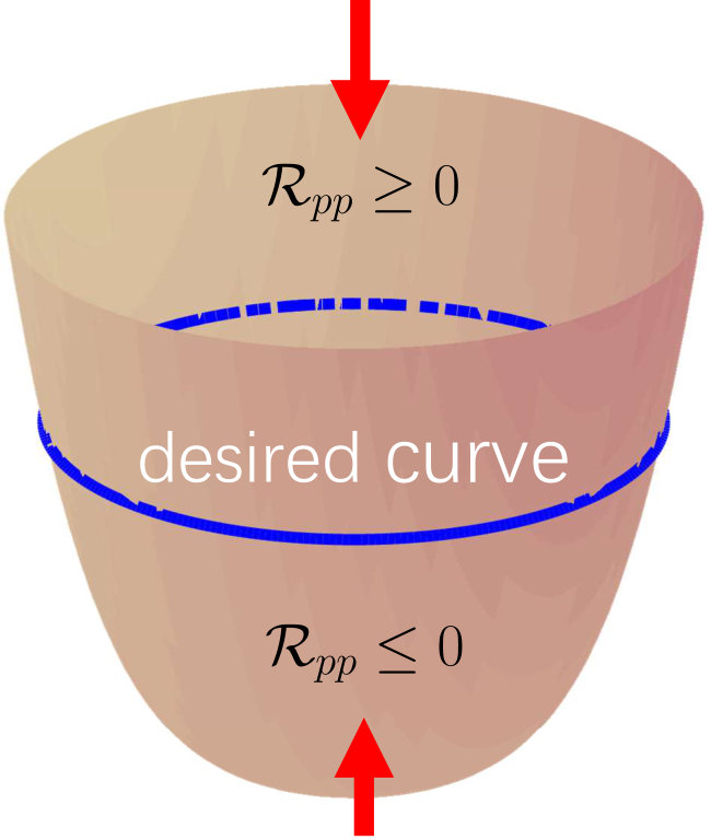 Figure 2
 Figure 3
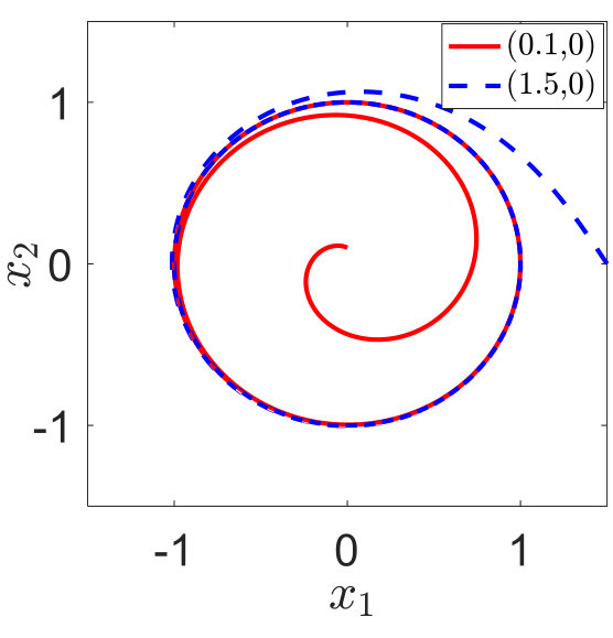 Figure 5
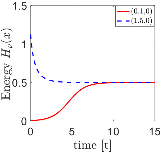 Figure 6
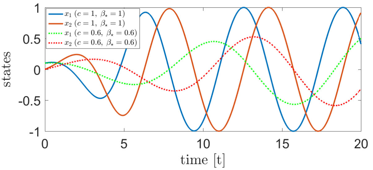 Figure 7
 Figure 8
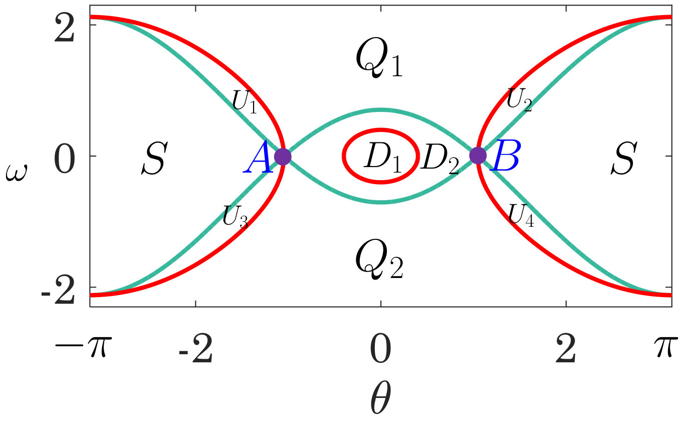 Figure 9
 Figure 10
 Figure 11
 Figure 12
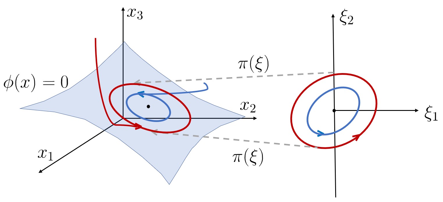 Figure 13
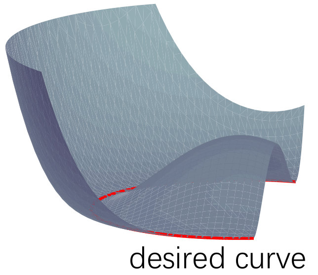 Figure 1
 Figure 2
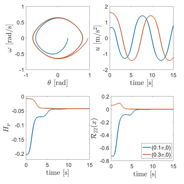 Figure 3
 Figure 17
 Figure 18
 Figure 19
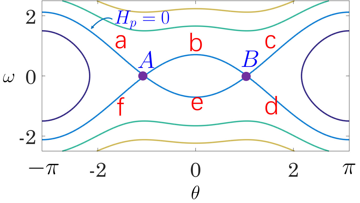 Figure 20
 Figure 21
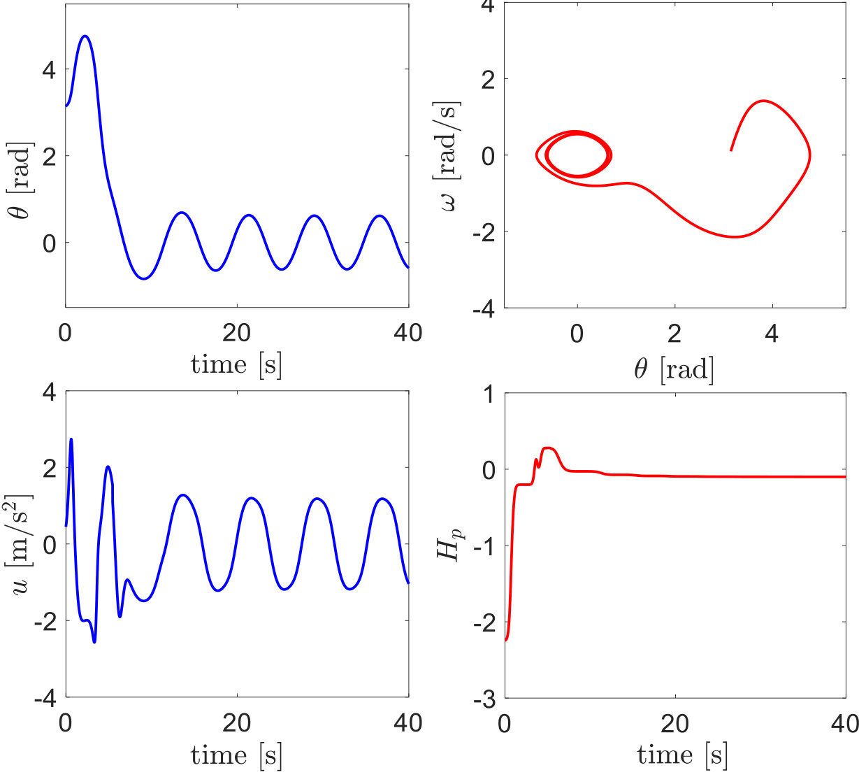 Figure 22
 Figure 23
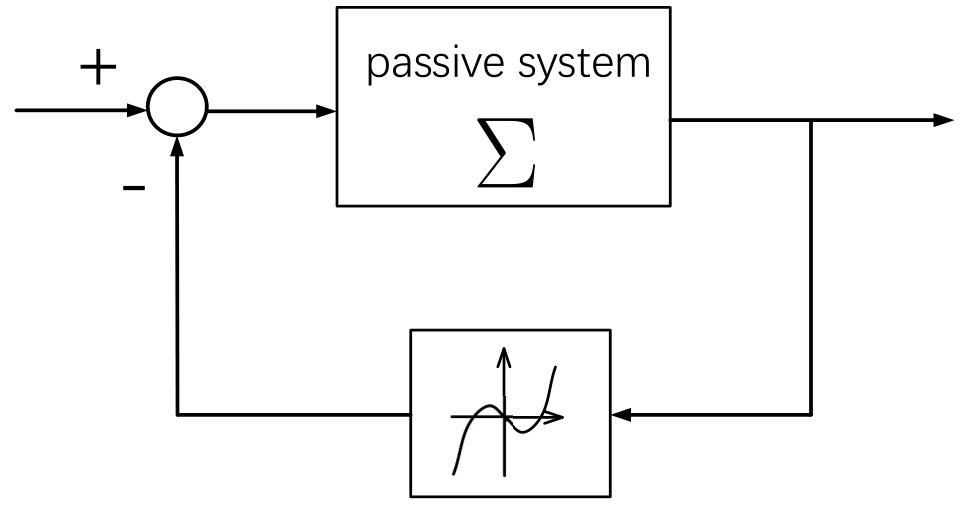 Figure 24
Peer Reviews
No public reviews on file for this paper yet. If you reviewed it on a platform where reviews are public (OpenReview, ICLR, NeurIPS, ICML), you can paste yours below so the community can read it here.
Videos
No videos yet. Explain this paper in a talk, walkthrough, or lecture? Add one.
Orbital Stabilization of Nonlinear Systems via Mexican Sombrero Energy Shaping and Pumping-and-Damping Injection
Bowen Yi [email protected]
Romeo Ortega [email protected]
Dongjun Wu [email protected]
Weidong Zhang [email protected] Department of Automation, Shanghai Jiao Tong University, 200240 Shanghai, China
Laboratoire des Signaux et Systèmes, CNRS-CentraleSupélec, 91192 Gif-sur-Yvette, France
Faculty of Control Systems and Robotics, ITMO University, St. Petersburg 197101, Russia
Abstract
In this paper we show that a slight modification to the widely popular interconnection and damping assignment passivity-based control method—originally proposed for stabilization of equilibria of nonlinear systems—allows us to provide a solution to the more challenging orbital stabilization problem. Two different, though related, ways how this procedure can be applied are proposed. First, the assignment of an energy function that has a minimum in a closed curve, i.e., with the shape of a Mexican sombrero. Second, the use of a damping matrix that changes “sign” according to the position of the state trajectory relative to the desired orbit, that is, pumping or dissipating energy. The proposed methodologies are illustrated with the example of the induction motor and prove that it yields the industry standard field oriented control.
keywords:
passivity-based control, nonlinear systems, orbital stabilisation, oscillator.
††thanks: Corresponding author: W. Zhang.
, , ,
1 Introduction
In many practical tasks the system under control is required to operate along periodic motions, i.e., walking and running robots, path following, rotating electromechanical systems, AC or resonant power converters, and oscillation mechanisms in biology. As clearly explained in [16, Section 8.4] the stability analysis of these behaviors can be recast as a standard equilibrium stabilization problem, but this leads to very conservative results. It is more convenient, instead, to invoke the notion of stability of an invariant set, where the latter is the closed orbit associated to the periodic solution. This approach leads to the important notion of orbital stability [16, Definition 8.2].
A large number of papers and books have been devoted to analysis of orbital stability of a given dynamical system, see e.g., [7, 11, 14]. However, there are only a few constructive tools available to solve the task of orbital stabilization of a controlled system. A popular approach to address this question is the virtual holonomic constraints (VHC) method, which has been tailored for mechanical systems of co-dimension one [17, 19, 27, 28]. In the VHC method a certain subspace of the state-space is rendered attractive and invariant, leading to a projected dynamics that behaves as oscillators. This is a particular case of the framework adopted in the immersion and invariance (I&I) technique, first reported for equilibrium stabilization in [2], and later extended for observer design and adaptive control in [3]. In [25] it has recently been shown that I&I can also be adapted for orbital stabilization, leading to a procedure that contains, as particular case, the VHC designs. The only modification done to the standard I&I technique is in the definition of the target dynamics that now should be chosen possessing periodic orbits, instead of an equilibrium at the desired point. A main drawback in both the VHC and I&I methods is that the steady-state behavior cannot be fixed a priori, but depends on the initial states, see [25, Remark 2] for a discussion on this matter.
An alternative approach to generate oscillations is reported in [26], where it is proposed to construct passive oscillators for Lure dynamical systems using “sign-indefinite” feedback static mappings, which is a mechanism similar to the pumping-and-damping injection discussed below. Unfortunately, since the analysis is carried out applying the center manifold theory—that is a local notion—the obtained oscillators are assumed to have small amplitudes. Orbital stabilization designs, for some particular controlled plants, have also been reported in [1, 11, 29].
The aim of this paper is to show that the widely popular interconnection and damping assignment passivity based control (IDA-PBC), originally proposed in [22, 23, 24] for stabilization of equilibria, can be easily be adapted to address the problem of orbital stabilization of general nonlinear systems. This leads to two new constructive solutions for this problem that—as usual in PBC—have a clear interpretations from the energy viewpoint. First, the assignment of an energy function that has a minimum in a closed curve, i.e., with the shape of a Mexican sombrero. Second, the use of a damping matrix that changes “sign” according to the position of the state trajectory relative to the desired orbit, that is, pumping or dissipating energy. As usual in all constructive nonlinear controller designs, the success of the proposed methods hinges upon our ability to solve a partial differential equation (PDE).
The remaining of the paper is organized as follows. Section 2 revisits the standard IDA-PBC. Section 3 introduces the problem formulation of orbital stabilization, followed by the constructive main results in Section 4. The application to the induction motor (IM) is reported in Section 5. Interestingly, we prove that the resulting controller exactly coincides with the industry standard direct field-oriented control (FOC) first proposed in [5]. In Section 6 the orbital stabilization of pendula is studied. The paper is wrapped-up with conclusions and future work in Section 7.
Notation. denotes the unit circle. Given a set and a vector , we denote , with , and . All mappings are assumed smooth. For a full-rank mapping with , we denote the generalized inverse as , and a full-rank left annihilator of . We define the gradient transpose operator as . When clear from the context the arguments of the mappings and the operator are omitted.
Caveat. An abridged version of this paper will be presented in [31].
2 Background on IDA-PBC
We consider in the paper systems written in the form
[TABLE]
with the state and the control and full rank. To solve the orbital stabilization problem we propose in the paper a variation of the IDA-PBC method [23], normally used for regulation tasks. The objective in IDA-PBC is to find a feedback control law such that the closed-loop dynamics takes a port-Hamitonian (pH) form, that is,
[TABLE]
with the desired Hamiltonian and
[TABLE]
the desired interconnection and damping matrices, respectively. The matching objective (2) is achieved if and only if the following PDE (in ) is solved
[TABLE]
If this is the case, the control law is given as
[TABLE]
In regulation tasks, has a unique minimum at the desired equilibrium and we choose the matrix to be positive semi-definite to inject the damping required to drive the trajectory towards the equilibrium. In this paper we show that, for orbital stabilization we select to have a minimum at the desired orbit—see Fig. 1. We will refer to this controller as Mexican sombrero energy assignment (MSEA) PBC.
An alternative option is to select the “sign” of to pump energy or inject damping according to the relative position of the state with respect to the desired orbit—this method is called energy pumping-and-damping (EPD)-PBC. A visual illustration is given in Fig. 2.
3 Problem Formulation
We are interested in the paper in the generation, via IDA-PBC, of periodic solutions which are asymptotically orbitally stable. That is,
[TABLE]
where the closed-loop vector field is given in (2), and the set is defined by its associated closed orbit
[TABLE]
is attractive.
We consider a particular case of periodic motion, which is defined as follows. First, split the state as , with . We also partition the matrices and conformally as
[TABLE]
Then, define the set as
[TABLE]
where is a constant vector and is a Jordan curve, given in implicit form as
[TABLE]
on which with a smooth function .
Remark 1**.**
It is important at this point to clarify the difference between our objective of orbital stabilization and the more classical set stabilization. The latter is satisfied ensuring , but this does not ensure that the desired periodic motion is generated. Indeed, if the set
[TABLE]
contains equilibrium points of the closed-loop dynamics the periodic motion is not generated. That is, we want to ensure that the closed-loop vector field (2) satisfies
[TABLE]
4 Main Results
We propose in this section two methods to solve the orbital stabilization problem posed above, MSEA and EPD-PBC, whose underlying philosophy is described in Section 2. Connections between these two methods are also given.
4.1 Mexican sombrero energy assignment PBC
The successful application of the IDA-PBC procedure described in Section 2 is guaranteed in MSEA with the following.
Assumption 1**.**
There are mappings (3) with and a function verifying
[TABLE]
which are solutions of the PDE (LABEL:pde), where we defined the function
There are two additional requirements to ensure the success of the MSEA design. First, a detectability-like condition to guarantee attractivity of the desired orbit. Second, to avoid the scenario discussed in Remark 1, we impose a constraint on the interconnection matrix, that ensures there are no equilibrium points in the set given in (5). These requirements are articulated in the assumptions of the following proposition.
Proposition 1**.**
Consider the system (1), verifying Assumption 1, in closed-loop with the control law with given in (2). Assume the following.
- H1
is the largest invariant set in the set
[TABLE]
for some . 2. H2
The (1,2)-element of may be parameterized as
[TABLE]
for some satisfying
Then, the closed-loop system is asymptotically orbitally stable.
Proof 1**.**
The closed-loop system takes the form
[TABLE]
From the isolated minimum condition of stated in (7), we conclude that the function has minima in the set . Consequently,
[TABLE]
for some . This shows that the set —containing the set —is non-empty.
From the closed-loop pH dynamics it is clear that
[TABLE]
implying the boundedness of . Together with (10), we conclude the Lyapunov stability of the closed-loop system with respect to . Thus, given a parameter , there always exists an invariant set such that Now, from the first equation of (10) we get
[TABLE]
Applying LaSalle’s invariance principle, taking into account the trajectory boundedness in , and the assumption H1, we prove the attractivity of , that is,
[TABLE]
The proof is completed establishing the existence of the periodic orbit, that is, verifying (6). Consider the term of the closed-loop dynamics:
[TABLE]
where we applied in the first identity the chain rule , and used assumption H2 in the third one. Considering that \nabla H(x)\big{|}_{x\in\mathcal{A}}=0, the residual dynamics is
[TABLE]
Now, from , we conclude that the set is invariant. To prove that the set is a periodic orbit, we compute the -norm of as
[TABLE]
With the additional Jordan curve assumption, the existence of a periodic orbit is verified, completing the proof.
Remark 2**.**
The minimum condition (7) implies that . Consequently, in view of condition (8), the mapping is singular along the orbit. However, the closed-loop dynamics and the feedback law (2) are well-defined everywhere. If the term is bounded along the orbit the condition (6) is violated. Consequently, the “infinite interconnection” condition H2 is necessary to ensure the orbit exists, otherwise we only achieve set stabilization—see Remark 1.
4.2 Energy pumping-and-damping PBC
In this subsection, we introduce an alternative orbital stabilization methodology: EPD-PBC—where the periodic orbit is enforced by regulating the energy level to a constant value. More precisely, we assume the total energy of the closed-loop can be decomposed as
[TABLE]
The function that defines the Jordan curve (4) is given as
[TABLE]
with the desired energy level for , which should be “above” the minimal value of , that is, it should satisfy
[TABLE]
To enforce the oscillation, the “sign” of the damping matrix changes according to the position of the state relative to the desired oscillation—whence, to the set . See Fig. 2.
Similarly to Assumption 1 for MSEA-PBC, in EPD-PBC we require that the PDE (LABEL:pde) is solvable, with an additional constraint on to implement the energy pumping-and-damping mechanism.
Assumption 2**.**
There exist functions and , which have isolated minima in and , respectively, and mappings (3), with
[TABLE]
where and the diagonal matrix satisfies the pumping-and-damping condition
[TABLE]
where is given in (12), and
[TABLE]
In EPD-PBC besides the detectability-like and the interconection conditions, we require a technical assumption to complete the proof. That is, , in order to “cut off” the energy flow between and partitions.
Proposition 2**.**
Consider the system (1), verifying Assumption 2, in closed-loop with the control law with given in (2). Assume the following.
- H3
{} is the largest invariant set in the set
[TABLE] 2. H4
The matrix satisfies
[TABLE] 3. H5
For some
[TABLE]
Then, the closed-loop system is asymptotically orbitally stable with respect to the orbit
Proof 2**.**
The closed-loop dynamics takes the form (9) with . From which it is clear that
[TABLE]
where we have used the assumption H4. Applying LaSalle’s invariance principle and using the assumption H3, we have
[TABLE]
For we have
[TABLE]
where we used again the assumption H4.
Consider the function we have
[TABLE]
where the inequality is the consequence of the pumping-and-damping condition (13). Invoking LaSalle’s invariance principle, the state ultimately converges into the largest invariant set of the set
[TABLE]
There are three cases of , namely,
- i)
;
- ii)
;
- iii)
and with
[TABLE]
First consider Case iii) with the definition
[TABLE]
We will prove that is not an invariant set by contradiction. Assume is invariant along the closed-loop dynamics. On the residual dynamics is
[TABLE]
with . Since , we have
[TABLE]
Assumption H4 ensures , hence from (15) we conclude that there are no equilibrium points in . From (15) we also conclude that
[TABLE]
Noticing the diagonal condition of , together with , for Case iii) and , we then have that contradicts the identity (16). Therefore, the set is not invariant, excluding the possibility of Case iii).
For Case i), from (14) we have
[TABLE]
Together with for all , it implies the invariance of Case i). For Case ii), it yields . In summary, the largest invariant set in is .
We consider the function and, for some small , it follows
[TABLE]
Therefore, the isolated equilibrium point is unstable. On the other hand, the set is attractive.
We proceed now to verify the existence of a periodic orbit. Since is a minimum of we have that
[TABLE]
If , the function qualifies as a Lyapunov function (for the dynamics with ). According to [6, Theorem 4.1], the set defines a Jordan curve. On the set the residual dynamics is
[TABLE]
We conclude , completing the proof.
Remark 3**.**
The condition H4 is similar, in nature, to H2, but excluding equilibria on the orbit . Noticing that on the desired orbit, only “finite interconnection” is adequate in the EPD method for the purpose of orbital stabilization. An example of energy regulation without adequate interconnection is given in our previous work [30], which solves the open problem—using smooth, time-invariant state-feedback to achieve almost global asymptotic regulation of three-dimensional nonholonomic systems.
Remark 4**.**
A trivial selection of the mapping is , but it is non-unique. This indeed provides an additional degree of freedom to solve the PDE, and the possibility to regulate the speed of convergence.
4.3 Comparison of MSEA-PBC and EPD-PBC
In this section we compare the two methods and clarify the parallel between them. To simplify the presentation we relabel the various mappings used in the methods with fonts mathcal () for MSEA-PBC and mathbf () for EPD-PBC. We have the following.
Proposition 3**.**
Consider the system (1), verifying all the assumptions in Proposition 1. Assume the matrix is diagonal, is a function of , and is non-zero. If the mapping can be decomposed as
[TABLE]
and then all the assumptions in Proposition 2 are satisfied by selecting the mappings111The notation represents the derivative of with respect to . We also have according to (17).
[TABLE]
and . Furthermore, the MSEA and EPD methods yield the same feedback law.
Proof 3**.**
We first verify the solvability of the matching PDEs—equivalently the coincidence of two closed-loop dynamics. The closed-loop dynamics in Proposition 1 is
[TABLE]
where we have used the assumption in the third equality. It is obvious that the closed-loop dynamics in Proposition 2 is exactly the same with the one in Proposition 1. The matching PDE in Proposition 2 is thus solvable.
Second, we will verify the assumptions in Proposition 2. With the decomposition (17), we have
[TABLE]
satisfying the convex properties of in Proposition 2. We then need to prove that there exists a point such that
[TABLE]
with . To this end, we notice that is diffeomorphic to the unit circle, and thus there exists a smooth mapping such that with and its inverse mapping is well-defined. By fixing , we then have
[TABLE]
for some small , where in the latter inequality we have used the continuity of the mapping and the fact . Thus we have verified the property of the Hamiltonian in Proposition 2.
To verify the condition (13), we have
[TABLE]
where we have used the assumption in the second implication, and the fact in the last one. Therefore, the equation (14) is satisfied. According to the property of , for sufficiently small we have for and if . It yields
[TABLE]
Thus, the pumping-and-damping condition—inequality (13)—has been proved. The remaining assumptions H3 and H4 are trivially verified.
4.4 Discussions
The following remarks are in order specifically emphasizing the connections between the proposed methods and existing methods.
Remark 5**.**
In the problem formulation, we impose the two-dimensional partition of . It may be argued to be peculiar and stringent. We should underscore that, in many cases, orbital stabilization tasks can be translated in to our case. We take the widely studied VHC method, though with a different mechanism from the proposed designs, for instance, and consider an Euler-Lagrange system with states and the generalized coordinates and velocities. The simplified control task in VHC is to stabilize the invariant manifold
[TABLE]
with some mapping , and guarantee the zero dynamics to admit non-trivial periodic solutions. It is clear that on the manifold we have The above-mentioned task appropriately adopts to our problem formulation with and the change of coordinate .
Remark 6**.**
A main drawback of VHC and I&I orbital stabilization technique is that the steady-state behavior cannot be fixed a priori, but depends on the initial states with a notable exception [19]. The drawback can be circumvented with the IDA methods, but with an additional difficulty in solving PDEs.
Remark 7**.**
In [1, 8, 13] a similar MSEA approach is adopted for some specific dynamical systems. In particular, in [8] the MSEA is imposed to the potential energy in a path following task for fully actuated mechanical systems.
Remark 8**.**
In [4] the pumping-and-damping injection is applied to stabilize pendula at the upright equilibrium almost globally. Some works on energy regulation of nonlinear systems, though not aiming at oscillation generation, can be found in [11, 12, 29].
Remark 9**.**
In [26] passive oscillators is constructed for Lure dynamical systems using “sign-indefinite” feedback static mappings, see Fig. 3. After assigning the linearized system with a unique pair of conjugated poles on the imaginary axis, the “sign-indefinite” feedback is adopted to regulate the energy achieving periodic oscillations. Indeed, [26, Theorem 2] can be regarded as an EPD controller. It should be underscored that the center manifold theory is applied in the analysis where the center manifold plays the exactly same role as the invariant manifold in VHC. Since the analysis of the latter is carried out applying the center manifold theory—whose nature is intrinsically local—the oscillators resulting from [26, Theorem 2] are assumed to have small amplitudes. On the other hand, they circumvent the daunting task of solving PDEs. Whereas, the proposed EPD method has the ability to shape behaviors of the closed-loop dynamics, making it instrumental in engineering practice.
Remark 10**.**
The assumptions in Proposition 4 on the equivalence between two proposed methods are relatively mild, namely, the diagonalization of and the decomposition of . Despite the equivalence, the realms of applicability of the methods are slightly different. For instance, if a controlled plant endows a pH form, it may be easier to generate oscillations via EPD without solving PDEs; on the other hand, for some systems it is simple to shape the Hamiltonian, e.g., fully-actuated mechanical systems, thus the MSEA method is preferred.
5 Induction Motor Example
5.1 Dynamic model and control objective
We consider the practical example of speed regulation of current-fed IMs. The normalized dynamics of the IM in the fixed frame is described by
[TABLE]
where is the rotor flux, is the rotor angular speed, is the constant load torque, is the rotor resistance, is the stator current, which is assumed to be the control and, without loss of generality, we have taken the rotor inertia to be equal to one—see [21, 18] for further details. To show the basic idea, we make the assumption that , which can be removed adding an integral in the control action [21, 18].
The control objective is to ensure the asymptotic orbital stabilization of the set
[TABLE]
where we introduced the notation , , defined the function
[TABLE]
and , are the desired (constant) references. Intuitively, we may fix the desired Hamiltonian as (25) then solving the PDE.
5.2 Orbital stabilization of the IM via MSEA-PBC
In the following proposition we show that the aforementioned regulation problem of IMs can be solved via MSEA-PBC.
Proposition 4**.**
Consider the fixed-frame current-fed IM model (21) and the target set (22), (23).
- P1
Assumption 1 is satisfied with the choices
[TABLE]
and
[TABLE] 2. P2
The controller (2) takes the form
[TABLE] 3. P3
All the assumptions of Proposition 1 are satisfied.
Consequently, the closed-loop system is asymptotically orbitally stable with respect to (22). Moreover, the convergence is exponential.
Proof 4**.**
The fact that Assumption 1 is satisfied with (24)-(26) is easily verified. Assumption H2 is also satisfied, with which evaluated in yields . The largest invariant set in is . Some basic Lyapunov analysis shows that the origin is an unstable equilibrium. According to Proposition 1, we conclude that the closed-loop system is almost globally asymptotically orbitally stable.
To establish the exponential orbital stability claim we refer to [15], where it is shown to be equivalent to prove that the transverse coordinate exponentially converges to . The proof of Proposition 1 shows that we can always find some invariant compact sets containing . In these compact sets, for some . Thus in the neighborhood of , we have
[TABLE]
then yielding the exponential convergence of to zero. Now we have
[TABLE]
where is an exponentially decaying term caused by . The Jordan curve implies in the neighborhood of , from which we conclude the exponential stability of the transverse coordinate .
Remark 11**.**
It can also be shown that the closed-loop system takes the pH form (9) with
[TABLE]
and satisfies all the assumptions of Proposition 2. Hence, the IM can be orbitally stabilized with the EPD-PBC also.
5.3 FOC of the IM is an MSEA-PBC
In this subsection we prove that the MSEA controller of Proposition 4 exactly coincides with the industry standard direct FOC first proposed in [5]—see also [18, Chapter 2.2] and [21, Chapter 11.2.1].
Corollary 1**.**
The MSEA controller (26) of Proposition 4 yields, after a state and input change of coordinates, the classical direct FOC.
Proof 5**.**
To prove that (26) coincides—modulo a coordinate change—with the direct FOC we introduce the change of coordinates
[TABLE]
that, applied to (21) (with ), yields the well-known current-fed IM dynamics in the rotating frame
[TABLE]
Now, we write (29) in polar coordinates as
[TABLE]
where we have defined
[TABLE]
It is easy to see from the equations above that the objective , which is equivalent to the asymptotic stabilization of the set222Notice that . , is achieved with the simple control
[TABLE]
with . This is the famous direct FOC for induction motors. It is a simple exercise to show that (26) is obtained applying to (30) the change of coordinates (28).
Remark 12**.**
It is interesting to note that, expressed in the rotating coordinates, the direct FOC does not generate a periodic orbit, but only ensures set stability.
Remark 13**.**
The application of the main idea of FOC of IMs for smooth regulation of Brockett’s non-holonomic integrator was first reported in [10], and later adopted in [9, 20] for control of nonholonomic systems.
6 Pendulum Example
6.1 Local design
We consider a benchmark in nonlinear control—the planar inverted pendulum, which is related to various applications, e.g., the attitude control of space boosters and walking robots. The normalized model given by [4]
[TABLE]
where and denote the angular position and velocity, and the input is the acceleration of the pivot. In this representation, the angles [math] and correspond to the upright and downright positions, respectively.
We are interested in asymptotically stabilizing the pendulum oscillating around its upright equilibrium. We define in the absence of the partition. The first design is a local result as follows.
Proposition 5**.**
Consider the model (31) in closed-loop with the control law
[TABLE]
with where , , and , the system is locally asymptotically orbitally stable. Furthermore, the angle ultimately oscillates between .
Proof 6**.**
We first define
[TABLE]
The closed loop takes the pH form (9) with333The Hamiltonian function is motivated by [4].
[TABLE]
The Hamiltonian function admits an isolated local minimal point at . Define and the periodic orbit is
[TABLE]
which is a Jordan curve.
The fact
[TABLE]
implies that the set
[TABLE]
is invariant for some . It is easy to verify the assumptions H3-H5 in the set . We complete the proof by applying Proposition 2.
We underscore that the level set containing two disconnected parts. Hence, the restriction is indispensable. We give the simulation results in Fig. 5 with initial values and , where and . In this figure we show the evaluation of the (2,2)-element of , illustrating the pumping-and-damping mechanism.
6.2 Almost global design
The following proposition is an almost global design.
Proposition 6**.**
Considering Proposition 5, if we select
[TABLE]
and
[TABLE]
then there exist such that the state asymptotically converges to the orbit or the saddles , almost globally on .
Proof 7**.**
The closed-loop is the same with the one in Proposition 5, but with a different function . We draw the curves of (the red one) and (the green one) in Fig. 5. They divide the manifold into 9 portions, where each set is defined as an open set. Intuitively, in the set
[TABLE]
the pumping-and-damping matrix is a pumping matrix, and in the set
[TABLE]
it acts as a damping one.
It is clear that
[TABLE]
We now consider three possible cases of the initial condition.
- In the set
[TABLE]
we have thus this connected set is a repeller. Noticing that the boundary of the set is the contour , thus all states in the set will leave into , which contains two equilibria and .
- It is also easy to show the set
[TABLE]
is invariant. In this set, we need to prove that the control law regulates the state to the desired energy level 444It should be noticed that the contour has two unconnected parts.. To this end, we define the function
[TABLE]
Its derivative along the closed-loop dynamics is
[TABLE]
with
[TABLE]
which is positive semi-definite in . We have the set equal to , and the equilibrium is unstable. Thus invoking LaSalle’s invariance principle, if the initial state is in , it will asymptotically converge to the desired periodic orbit.
- For the set or the set , it is relatively complicated. For convenience, we define the set
[TABLE]
Since the set is a repeller, the states which star in have two possible trajectories:
3a)
converging to the compact set , and then it can be analyzed as case 2).
3b)
staying in the set for all .
Following the proof in [4] with some complicated analysis, we can prove the energy dissipation in thus ruling out the case 3b) except two equilibria and . It completes the proof.
Fig. 6 gives the simulation results to illustrate Proposition 6 with the , and . The figure illustrates the almost global property with the angle ultimately oscillating between .
7 Concluding Remarks
It has been shown that the IDA-PBC design methodology can be adapted to address the problem of orbital stabilization of nonlinear systems. We propose two different, but related, IDA-PBC designs: MSEA and EPD—whose application, as usual in IDA, requires the solution of a PDE. In the former, the closed-loop Hamiltonian function is shaped to have minima at the desired orbit. For the latter, we regulate the energy to a desired value using a pumping-and-damping dissipation matrix. To ensure asymptotic orbital stability, and not just set attractivity, some constraints are imposed on the interconnection matrix. We then establish connections between the above-mentioned methods.
Currently research is carried out in the following directions.
- •
The problem of path following—in a time parameterization-free manner—for mechanical systems. It has been observed that this is closely related to the orbital stabilization problem studied in this paper.
- •
The connection between the proposed method and the indirect version of FOC is still an open, and interesting, topic.
- •
Application of the proposed methods to solve some periodic motion control problems in mechanical and power electronic systems, e.g. in walking robots and AC (or resonant) power converters.
{ack}
This paper is supported by the NSF of China (61473183, U1509211, 61627810), National Key R&D Program of China (SQ2017YFGH001005), China Scholarship Council and by the Government of the Russian Federation (074U01), the Ministry of Education and Science of Russian Federation (GOSZADANIE 2.8878.2017/8.9, grant 08-08).
The reference list from the paper itself. Each links out to its DOI / PubMed record.
- 1[1] J. Aracil, F. Gordillo and E. Ponce, Stabilization of oscillations through backstepping in high-dimensional systems, IEEE Trans. Automatic Control , vol. 50, pp. 705-710, 2005.
- 2[2] A. Astolfi and R. Ortega, Immersion and invariance: A new tool for stabilisation and adaptive control of nonlinear systems, IEEE Trans. Automatic Control , vol. 48, pp. 590-606, 2003.
- 3[3] A. Astolfi, D. Karagiannis and R. Ortega, Nonlinear and Adaptive Control with Applications , Springer-Verlag, Berlin, Communications and Control Engineering, 2008.
- 4[4] K.J. Astrom, J. Aracil and F. Gordillo, A family of smooth controllers for swinging up a pendulum, Automatica , vol. 44, pp. 1841-1848, 2008.
- 5[5] F. Blaschke, The principle of field orientation as applied to the new TRANSVEKTOR closed loop control system for rotating field machines, Siemens Review , vol. 39, pp. 217-220, 1972.
- 6[6] C.I. Byrnes, On Brockett’s necessary condition for stabilizability and the topology of Liapunov functions on ℝ n superscript ℝ 𝑛 \mathbb{R}^{n} , Communications in Information and Systems , vol 8, pp. 333-352, 2008.
- 7[7] D. Cheban, Global Attractors of Non-Autonomous Dissipative Dynamical Systems , , World Scientifc Publishing Co. Pte. Ltd., Singapore, 2004.
- 8[8] V. Duindam and S. Stramigioli, Port-based asymptotic curve tracking for mechanical systems, European Journal of Control , vol. 10, pp. 411-420, 2004.