Lattice-depth measurement using continuous grating atom diffraction
Benjamin T. Beswick, Ifan G. Hughes, Simon A. Gardiner

TL;DR
This paper introduces a novel method for measuring optical lattice depths by analyzing high-amplitude oscillations in atomic diffraction patterns, which are robust against temperature variations, enabling simultaneous temperature and lattice depth determination.
Contribution
The authors develop an analytic model for lattice-depth measurement using atomic diffraction oscillations, extending it to finite temperatures and initial momenta, facilitating more accurate and robust characterization.
Findings
Analytic formula for zero-temperature oscillations
Extension of model to finite-temperature response
Steady-state solution enabling simultaneous measurement of lattice depth and temperature
Abstract
We propose a new approach to characterizing the depths of optical lattices, in which an atomic gas is given a finite initial momentum, which leads to high amplitude oscillations in the zeroth diffraction order which are robust to finite-temperature effects. We present a simplified model yielding an analytic formula describing such oscillations for a gas assumed to be at zero temperature. This model is extended to include atoms with initial momenta detuned from our chosen initial value, before analyzing the full finite-temperature response of the system. Finally we present a steady-state solution to the finite-temperature system, which in principle makes possible the measurement of both the lattice depth, and initial temperature of the atomic gas simultaneously.
Click any figure to enlarge with its caption.
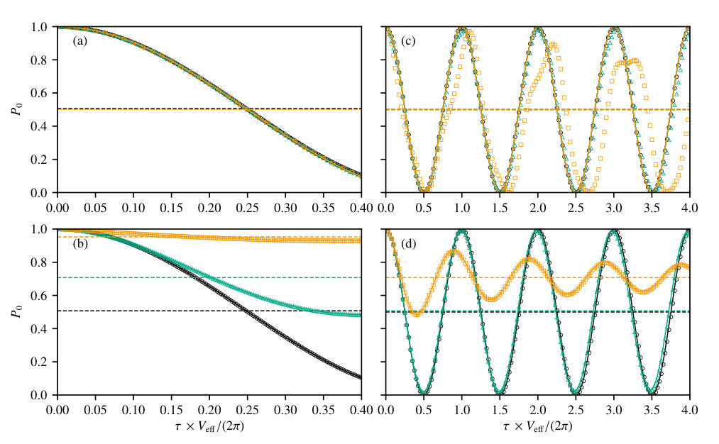 Figure 1
 Figure 2
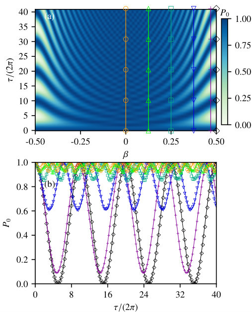 Figure 3
 Figure 4
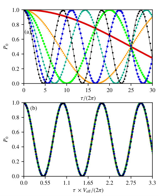 Figure 5
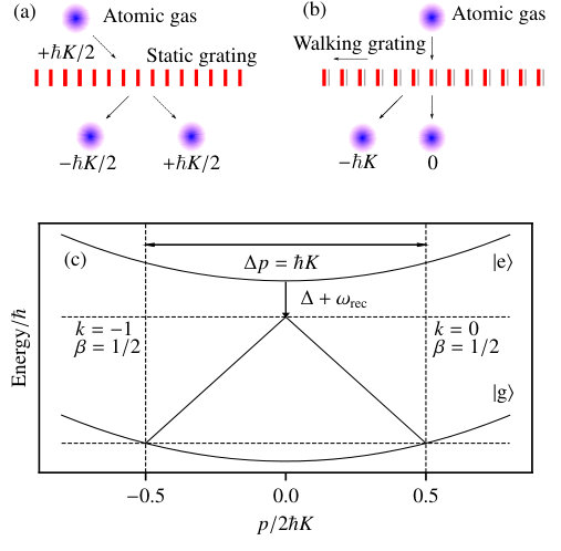 Figure 6
 Figure 7
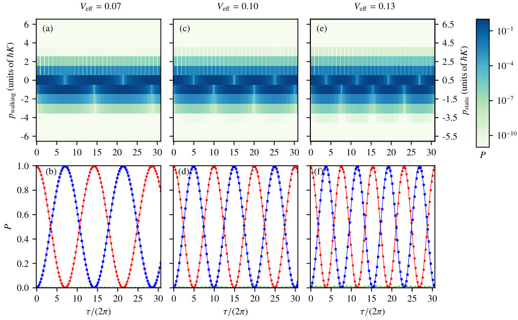 Figure 8
 Figure 9
 Figure 10
Peer Reviews
No public reviews on file for this paper yet. If you reviewed it on a platform where reviews are public (OpenReview, ICLR, NeurIPS, ICML), you can paste yours below so the community can read it here.
Videos
No videos yet. Explain this paper in a talk, walkthrough, or lecture? Add one.
Lattice-depth measurement using continuous grating atom diffraction
Benjamin T. Beswick
Ifan G. Hughes
Simon A. Gardiner
Joint Quantum Centre (JQC) Durham–Newcastle, Department of Physics, Durham University, Durham DH1 3LE, United Kingdom
Abstract
We propose a new approach to characterizing the depths of optical lattices, in which an atomic gas is given a finite initial momentum, which leads to high amplitude oscillations in the zeroth diffraction order which are robust to finite-temperature effects. We present a simplified model yielding an analytic formula describing such oscillations for a gas assumed to be at zero temperature. This model is extended to include atoms with initial momenta detuned from our chosen initial value, before analyzing the full finite-temperature response of the system. Finally we present a steady-state solution to the finite-temperature system, which in principle makes possible the measurement of both the lattice depth, and initial temperature of the atomic gas simultaneously.
I Introduction
There is much interest in the precise measurement of optical lattice Morsch and Oberthaler (2006) depths in the field of atomic physics, particularly for accurate determination of transition matrix elements Mitroy et al. (2010); Arora et al. (2011); Henson et al. (2015); Leonard et al. (2015); Clark et al. (2015), better knowledge of these matrix elements can be used to improve the black body radiation correction for ultraprecise atomic clocks Safronova et al. (2011); Sherman et al. (2012), and allows quantitative modeling of atom-light interaction Whiting et al. (2016). Other areas of interest include atom interferometry Cronin et al. (2009); A. Miffre and M. Jacquey and M. Büchner and G. Trénec and J. Vigué (2006) and many body quantum physics Bloch et al. (2008); Jo et al. (2012), where knowledge of the lattice depth is essential for interpreting experimental results.
Commonly used lattice depth measurement schemes include Kapitza–Dirac scattering Cahn et al. (1997); Gadway et al. (2009); Birkl et al. (1995); Cheiney et al. (2013); Jo et al. (2012), parametric heating Friebel et al. (1998), Rabi oscillations Ovchinnikov et al. (1999), and, more recently, the sudden phase shift method Cabrera-Gutiérrez et al. (2018). For the case of a weak lattice ( for any atom, where is the lattice depth and is the atomic recoil energy), methods based on multipulse atom diffraction have been explored Herold et al. (2012); Kao et al. (2017), with a view to reducing signal-to-noise considerations in the measurement of the resultant diffraction patterns. In previous work we have presented improved models for the expected multipulse diffraction patterns for a given lattice depth. We have also noted that when considering a gas with initial momentum , the functional form of these models is markedly simpler and therefore easier to fit to data to make an accurate measurement of the lattice depth Beswick et al. (2019).
In this paper we explore such a measurement scheme for a lattice which is not pulsed but instead continuously present throughout the experimental sequence, which we show to be more robust to finite-temperature effects than a multipulse approach. In Sec. II, we describe our model system and experimental considerations. In Sec. III, we introduce a simplified analytic approach for determining the time evolution of the atomic population in the zeroth diffraction order, and make a comparison to exact numerical calculations. Finally, in Sec. IV, we present an approximate analytic model for the finite-temperature response of the system, and discuss how these may be used to determine both the lattice depth and initial temperature of the atomic gas.
II Model system: Atomic gas in an optical grating
II.1 Experimental setup and Hamiltonian
We consider a two-level atom in an assumed noninteracting Bose-Einstein condensate exposed to a far off resonance optical grating, the Hamiltonian of which is given by Eq. (1):
[TABLE]
where is the momentum operator along the lattice axis, is the lattice depth, is twice the laser wavenumber , is the atomic mass and is the phase velocity of the grating in the direction (=0 for a static grating). For the simpler case of a static grating, we consider a BEC initially prepared in a momentum state with .111The initial momentum is chosen with a view to creating population oscillations between the zeroth and first diffraction orders with a strong sinusoidal character, as suggested in Beswick et al. (2019). As shown in Fig. 1(a), the BEC is diffracted by the static optical grating for a time , before a time of flight measurement interrogates the population of the gas in each of the allowed momentum states. In principle there is an infinite ladder of such states, each separated by integer multiples of Bienert et al. (2003); Beswick et al. (2016), though here we show only the zeroth and first diffraction orders. We note that an initial state can be achieved for instance by Bragg diffraction, or equivalently we may prepare the BEC in a state with and impart an appropriately tuned time-dependent phase to the standing wave as in Fig. 1(b). We show this equivalency in Sec. II.2 below.
II.2 Gauge transformations and momentum kicks
The Hamiltonian of Eq. (1) can be transformed to a frame comoving with the walking grating by use of the unitary transformation
[TABLE]
where we have chosen for convenience. Using and . This transformation yields:
[TABLE]
The Hamiltonian of Eq. (3) describes the system in a frame moving with velocity , therefore, a gas moving with velocity in the moving frame appears to move with velocity in the lab frame. Conversely, a gas moving with velocity in the comoving frame, moves with velocity in the lab frame. Choosing yields the case in Fig. 1(a), while with , we have the situation shown in Fig. 1(b).
The spatial periodicity of Eq. (3) allows us to invoke Bloch theory Ashcroft and Mermin (1976), by rewriting the momentum operator in the following basis:
[TABLE]
We may speak of as the discrete part of the momentum, and as the continuous part or quasimomentum Bach et al. (2005). Here is a conserved quantity, as such, only momentum states separated by integer multiples of are coupled Bienert et al. (2003); Beswick et al. (2016). This simplification allows us to construct the time evolution operator for a lattice pulse of duration from the lattice Hamiltonian (3) as follows:
[TABLE]
in which is simply a scalar value such that overall phases which depend solely on can be neglected. Here is the dimensionless lattice depth, and is the rescaled time.
By using Eq. (5) to calculate , the population in each discrete momentum state following an evolution for a rescaled time of is given by the absolute square of the coefficients . In this paper we employ the well-known split-step Fourier approach Daszuta and Andersen (2012); Beswick et al. (2016) to determine , as well as an analytic approach based on a simpler two-state model.
The dynamics of a single atom in the BEC standing-wave system can be understood in terms of the scattering process given by the semiclassical energy diagram of Fig. 1(c) (see also Martin et al. (1988); Giltner et al. (1995); bor (1997); Kozuma et al. (1999); Gupta et al. (2001)). A two-level atom begins in a state with momentum , before absorbing a photon with momentum , and subsequently emits a second photon with the momentum . This is the only scattering process which classically conserves energy, whilst also conserving the quasimomentum. We therefore expect that scattering into states with momentum ought to be strongly suppressed even under the fully quantum time evolution. We explore this simplified picture in Sec. III.
III Reduction to an effective 2-state system
III.1 Simplification
We may test the conjecture that population transfer into states with or is strongly suppressed by computing the full time evolution of the system numerically, the results of such calculations on an exhaustive basis of momentum states are displayed in Fig 2. Over the 13 basis states displayed, we can clearly see that, though population transfer into higher order modes does occur, the oscillation of population between the and states is the dominant process in the system. We therefore expect that a representation of the system in a truncated momentum basis composed of only these two states ought to capture the essential dynamics, and explore this simplified two-state model below.
III.2 Two-state model analytics
We may represent the Hamiltonian (3) in the subspace using the following two-state momentum basis:
[TABLE]
yielding:
[TABLE]
We recognize Eq. (7) as a Rabi matrix with zero detuning, the eigenvectors and eigenvalues of which are well known Barnett and Radmore (1997), and can be used to straightforwardly determine the time evolution of the population in the and states, respectively:
[TABLE]
as outlined in Appendix A. This analytic result is compared to our exact numerics in Figs. 2 and 3, both of which show excellent agreement for a wide range of experimentally relevant values of the effective lattice depth . We note in particular that the form of Eqs. (8a) and (8b) is such that there is an exact universality between and , which is elucidated in Fig. 3(b), where all population curves fall on top of each other.
IV Finite-temperature response
IV.1 Other values of
In the following section we consider the effect of evolving initial states with quasimomentum different to in order to gain insight into the dynamics of a finite-temperature gas. Numerically, this is achieved by computing the evolution of an initial state under the time evolution operator (5). We make the assumption from the outset that the initial momentum distribution of the gas (centred at ) spans less than half of each of the and Brillouin zones for a static grating (or falls within the Brillouin zone with a momentum distribution centered on for a walking grating). Our results in this low temperature regime are displayed in Fig. 4, which indicates a Brillouin zone with high amplitude but low-frequency oscillations in the population of the zeroth diffraction order centered around , and low amplitude but rapidly oscillating solutions as is detuned from this value.
We may also use our simplified semiclassical model of Sec. III to derive an approximate analytic result for the same calculation, in which the quasimomentum is encoded as a detuning to be included in our initial Rabi model of Eq. (7). These additions yield the following Hamiltonian matrix:
[TABLE]
in which is now a free parameter. The time evolution of the zeroth diffraction order population governed by this matrix can be found using the approach given in Appendix B, thus:
[TABLE]
which is similar to the result reported in Gadway et al. (2009) for a zero temperature gas, and agrees excellently with the exact numerics for physically relevant parameters as shown in Fig. 4. We therefore expect that thermal averaging of this result should produce an accurate description of the full finite-temperature response.
IV.2 Finite temperature analysis
To find the finite temperature response of the system we weight the contribution of Eq. (10) for each individual quasimomentum subspace according to the Maxwell-Boltzmann distribution:
[TABLE]
where the dimensionful temperature is given by Saunders et al. (2007). Mathematically this corresponds to the integral:
[TABLE]
Inserting Eqs. (11) and (10), we have:
[TABLE]
where we have introduced , and for simplicity. The exponential and trigonometric terms can be power expanded, and the integral (13) solved term by term, giving:
[TABLE]
where , and (see Appendix C). Equation (14) can in principle be solved numerically by recursively populating the elements of a sufficiently large pair of , vectors and matrix, though the elements of the vectors will grow with and respectively unless and are sufficiently small, and this condition is only satisfied for certain experimentally relevant regimes. Nonetheless, Eq. (14) yields some insight when expressed as a sum over derivatives of sinc functions (see Appendix D):
[TABLE]
With , Eq. (15) reduces to the zero temperature result of Eq. (8a), as such we should expect the finite temperature behavior of the system to be captured in terms with . Though the full sum over is always convergent, the presence of the term guarantees that all individual terms with diverge, meaning that a preferred truncation of the sum is not obvious.
However, given the well-behaved nature of the integrand, Eq. (13) can be straightforwardly integrated numerically, for instance using the trapezium rule. We compare this numerical integration to our full finite-temperature numerics in Fig. 5, which shows excellent agreement across a large range of initial momentum widths in the weak lattice regime [Figs. 5 (a),(b)], and for in the strong lattice regime [Fig. 5 (d)]. However, for [Fig. 5 (c)] the agreement is relatively poor, as in this regime the semiclassically motivated two-state model is no longer valid. We therefore expect that numerically fitting Eq. (13) to experimental data, with and as free parameters, would give an accurate value of the effective lattice depth, if the time is known to high precision and the lattice depth is sufficiently small.
Further, we note that using standard integral results, we may also extract the steady state solution to Eq. (13) as :
[TABLE]
which depends only on . Here, ‘Erfc’ is the complementary error function Hughes and Hase (2010).222When evaluating Eq. (16) for physically relevant values of , the exponential term becomes large as the error function takes a correspondingly such that remains bounded between 0 and 1. This complication can present a problem for numerical evaluation using standard numerical routines. In practice, we numerically implement Eq. (16) exclusively in terms of rational numbers in Mathematica, before requesting a numerical evaluation to a specified precision. In essence, by measuring the steady state population experimentally, and numerically fitting Eq. (16), can be straightforwardly determined and substituted into Eq. (13), leaving a fit in only one parameter . The steady state population can be found either by allowing the atomic gas to evolve in the lattice for a sufficiently long time, or taking the average value of in time for an appropriate number of oscillations. In fact, this improved fitting approach not only allows , and therefore the effective lattice depth to be determined more accurately, but also allows the initial effective temperature to be determined from .
V Conclusions
We have presented a simplified model system yielding an analytic zero-temperature formula for the evolution of the zeroth diffraction order population, and demonstrated the validity of this approach across a wide range of lattice depths. We have extended this model to incorporate finite-temperature effects and discussed from where they arrive mathematically. We have shown that there is excellent agreement between this analytic model and exact numerical calculations if the lattice depth is sufficiently small, and shown that a steady state solution exists, which may be useful for determining the lattice depth and initial temperature of a gas from a single set of population measurements. With regard to potential experimental implementations, we note that the phase velocity of a walking optical lattice can be calibrated extremely precisely, however, does require optical elements to be in place which will reduce the intensity of the laser beam and therefore the lattice. The alternative is to impart a specified momentum to an initially stationary BEC; it is unlikely that this can be achieved with the same level of precision, however there is no need for any additional optical elements affecting the lattice depth.
Acknowledgements.
B.T.B., I.G.H., and S.A.G. thank the Leverhulme Trust research program grant RP2013-k-009, SPOCK: Scientific Properties of Complex Knots for support. We would also like to acknowledge helpful discussions with Andrew R. MacKellar.
Appendix A Derivation of the two-state model
To calculate the time-evolution of the population in the zeroth diffraction order, we construct the time evolution operator in the momentum basis from the Hamiltonian of Eq. (7), reproduced here for convenience:
[TABLE]
The diagonal terms simply represent an energy shift that can be transformed away, thus the eigenvalues of Eq. (7) can simply be read from the off-diagonal: . We may now solve the eigenvalue equation:
[TABLE]
Equation (18) leads directly to , yielding eigenvectors:
[TABLE]
We may now construct our initial condition in the energy basis, in which the matrix representation of the time evolution operator
[TABLE]
is diagonal:
[TABLE]
The time evolution of the population in the zeroth diffraction order is given by:
[TABLE]
which corresponds to Eq. (8a).
Appendix B Derivation of dependent two-state model
To calculate the time-evolved population for a given quasimomentum subspace, we follow the same procedure as in Appendix A. Equation (9), reproduced here for convenience
[TABLE]
is nothing other than a Rabi matrix, the eigenvalues of which are , and the corresponding eigenvectors:
[TABLE]
where . This leads directly to:
[TABLE]
We may now simply calculate the time-evolved state from the action of the time evolution operator
[TABLE]
on this initial state thus:
[TABLE]
Here we have introduced . The time-evolved population in the zeroth diffraction order for a given subspace is then given by:
[TABLE]
which corresponds to Eq. (10).
Appendix C Derivation of finite-temperature matrix equation
To derive the matrix equation for the finite-temperature response of the zeroth diffraction order population, we begin from Eq. (12), into which we insert Eqs. (11) and (10), yielding:
[TABLE]
where we have introduced . For simplicity, we now refer to , the population in the state. The sinusoidal term can be rewritten using , thus:
[TABLE]
where we have used the fact that the integrand is an even function. The term in can then be power expanded, leading to:
[TABLE]
such that the square root in the argument no longer appears, and the term can be binomially expanded thus:
[TABLE]
Further, introducing , the remaining integral can be rewritten as:
[TABLE]
which, when substituted into Eq. (28) leads to:
[TABLE]
Finally, noting that , Eq. (29) can be rewritten, thus:
[TABLE]
or, equivalently, with and :
[TABLE]
which corresponds to Eq. (14).
Appendix D Expression of Eq. (14) in terms of Sinc functions
Equation (30) can be rewritten as:
[TABLE]
where we have used and . We now introduce and re-index the sum in , yielding:
[TABLE]
Expanding the factorial terms in and rearranging in in the following way:
[TABLE]
which we recognize can be expressed as a derivative in , thus:
[TABLE]
Equation (31) can be rewritten:
[TABLE]
such that the sum in can now be recognized as a sinusoidal term, yielding:
[TABLE]
Reintroducing leads to:
[TABLE]
Equivalently,
[TABLE]
which corresponds to Eq. (15).
The reference list from the paper itself. Each links out to its DOI / PubMed record.
- 1Morsch and Oberthaler (2006) Oliver Morsch and Markus Oberthaler, “Dynamics of Bose-Einstein condensates in optical lattices,” Rev. Mod. Phys. 78 , 179 (2006) . · doi ↗
- 2Mitroy et al. (2010) J. Mitroy, M. S. Safronova, and Charles W. Clark, “Theory and applications of atomic and ionic polarizabilities,” J. Phys. B: At. Mol. Opt. Phys. 43 , 202001 (2010) .
- 3Arora et al. (2011) Bindiya Arora, M. S. Safronova, and Charles W. Clark, “Tune-out wavelengths of alkali-metal atoms and their applications,” Phys. Rev. A 84 , 043401 (2011) . · doi ↗
- 4Henson et al. (2015) B. M. Henson, R. I. Khakimov, R. G. Dall, K. G. H. Baldwin, Li-Yan Tang, and A. G. Truscott, “Precision measurement for metastable helium atoms of the 413 nm tune-out wavelength at which the atomic polarizability vanishes,” Phys. Rev. Lett. 115 , 043004 (2015) . · doi ↗
- 5Leonard et al. (2015) R. H. Leonard, A. J. Fallon, C. A. Sackett, and M. S. Safronova, “High-precision measurements of the Rb 87 superscript Rb 87 {}^{87}\mathrm{Rb} D-line tune-out wavelength,” Phys. Rev. A 92 , 052501 (2015) . · doi ↗
- 6Clark et al. (2015) Logan W. Clark, Li-Chung Ha, Chen-Yu Xu, and Cheng Chin, “Quantum Dynamics with Spatiotemporal Control of Interactions in a Stable Bose-Einstein Condensate,” Phys. Rev. Lett. 115 , 155301 (2015) . · doi ↗
- 7Safronova et al. (2011) M. S. Safronova, M. G. Kozlov, and Charles W. Clark, “Precision calculation of blackbody radiation shifts for optical frequency metrology,” Phys. Rev. Lett. 107 , 143006 (2011) . · doi ↗
- 8Sherman et al. (2012) J. A. Sherman, N. D. Lemke, N. Hinkley, M. Pizzocaro, R. W. Fox, A. D. Ludlow, and C. W. Oates, “High-accuracy measurement of atomic polarizability in an optical lattice clock,” Phys. Rev. Lett. 108 , 153002 (2012) . · doi ↗