A full controller for a fixed-wing UAV
Gerardo Flores, Alejandro Flores, Andr\'es Montes de Oca

TL;DR
This paper introduces a nonlinear control law for fixed-wing UAVs that integrates path-following and longitudinal control, ensuring stability and robustness using only available state information for easy implementation.
Contribution
The proposed control law uniquely combines path-following and longitudinal control in a single, robust, and easily implementable framework tailored for commercial autopilots.
Findings
Closed-loop system is globally asymptotically stable.
Controller is robust to external disturbances.
No additional sensors or observers are required.
Abstract
This paper presents a nonlinear control law for the stabilization of a fixed-wing UAV. Such controller solves the path-following problem and the longitudinal control problem in a single control. Furthermore, the control design is performed considering aerodynamics and state information available in the commercial autopilots with the aim of an ease implementation. It is achieved that the closed-loop system is G.A.S. and robust to external disturbances. The difference among the available controllers in the literature is: 1) it depends on available states, hence it is not required extra sensors or observers; and 2) it is possible to achieve any desired airplane state with an ease of implementation, since its design is performed keeping in mind the capability of implementation in any commercial autopilot.
Click any figure to enlarge with its caption.
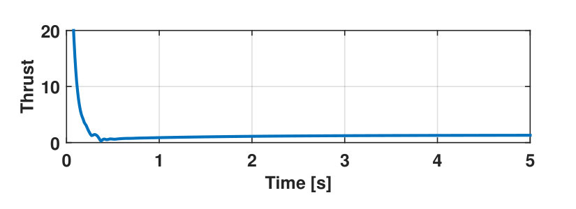 Figure 1
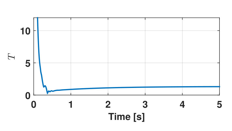 Figure 2
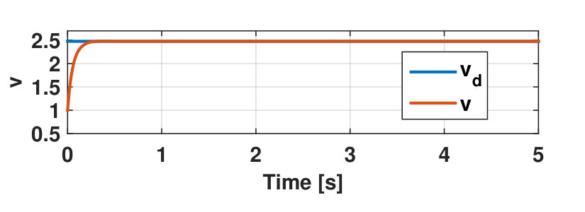 Figure 3
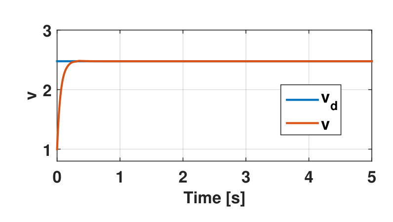 Figure 4
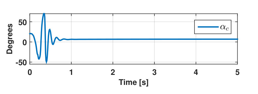 Figure 5
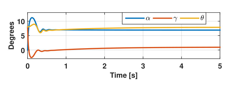 Figure 6
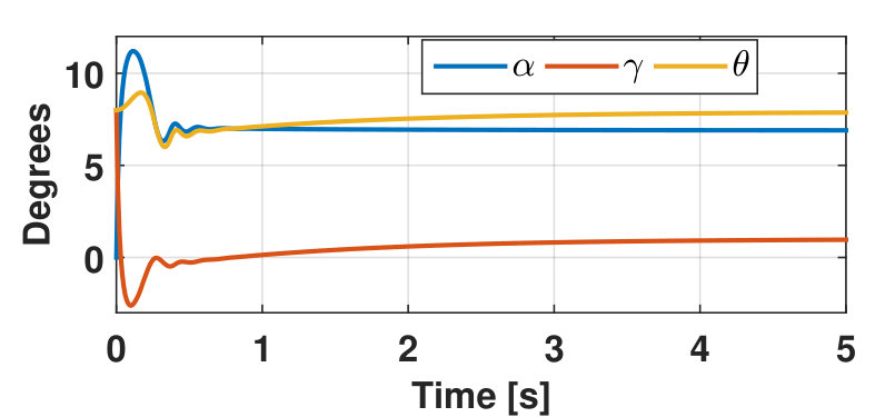 Figure 7
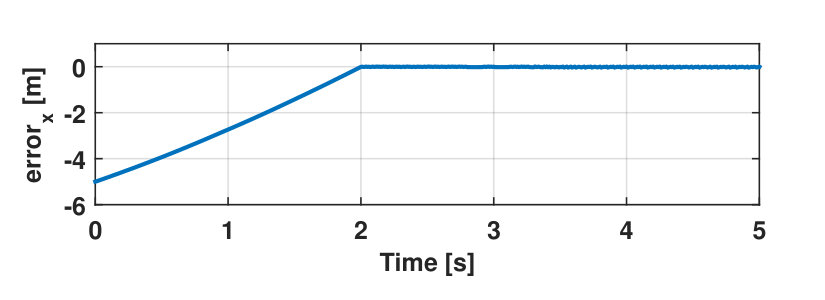 Figure 8
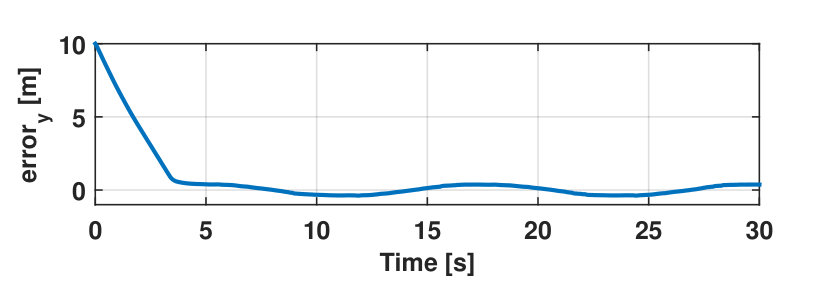 Figure 9
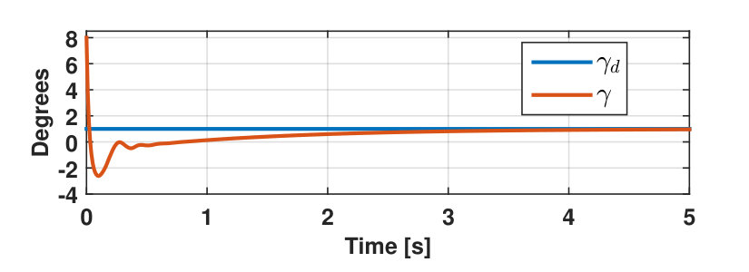 Figure 10
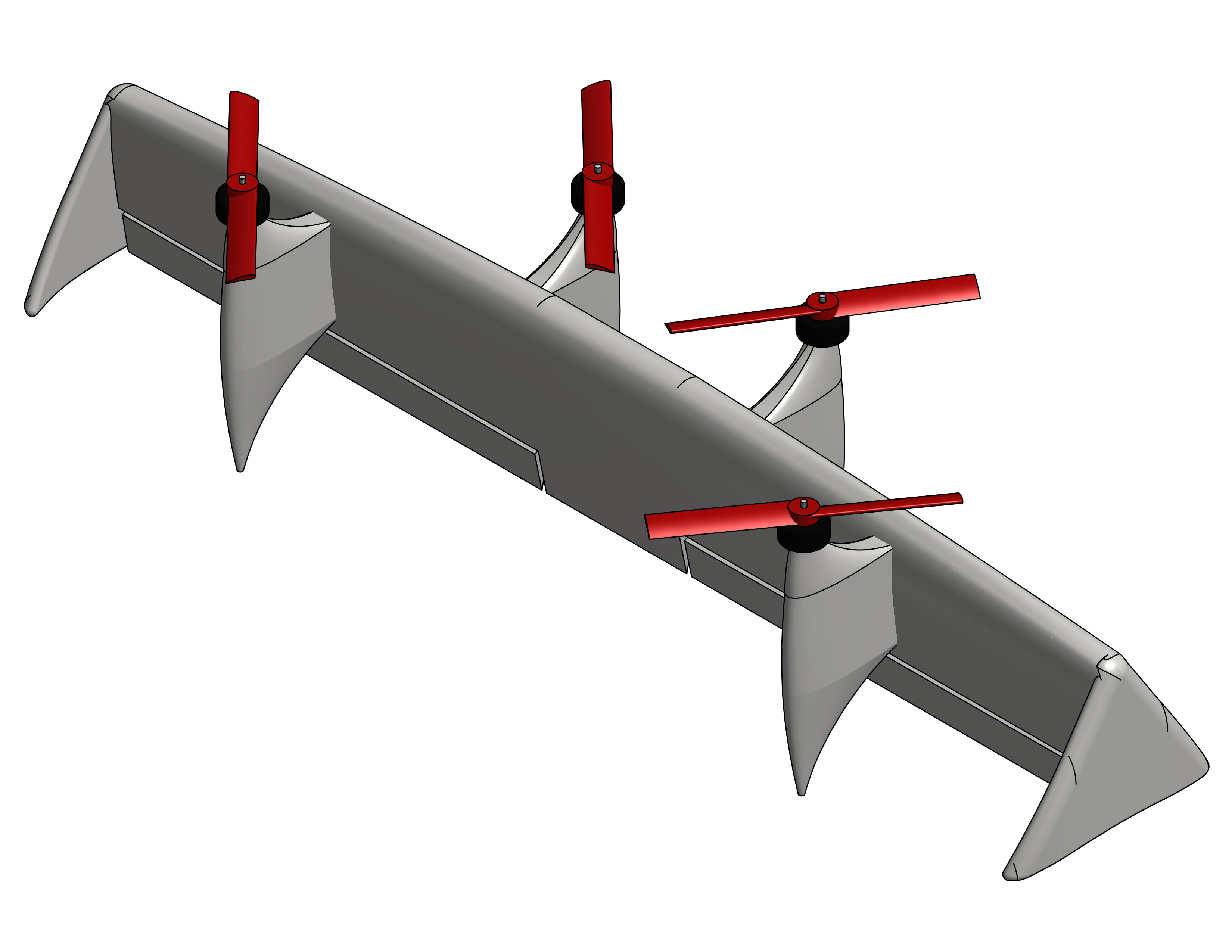 Figure 11
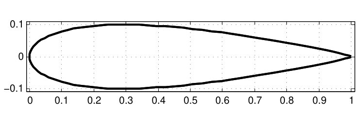 Figure 12
 Figure 13
 Figure 14
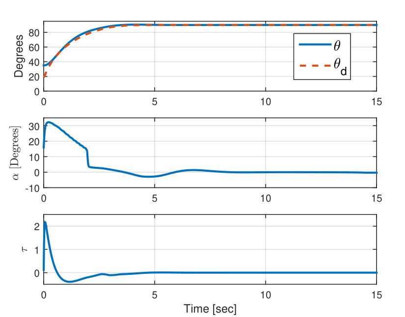 Figure 15
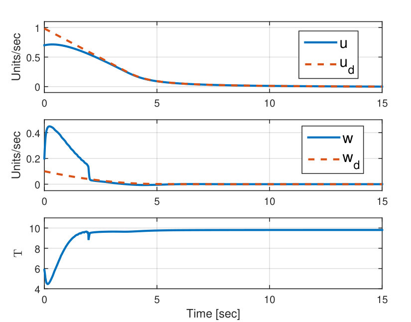 Figure 16
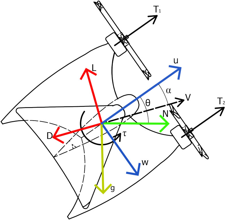 Figure 17
 Figure 18
 Figure 19
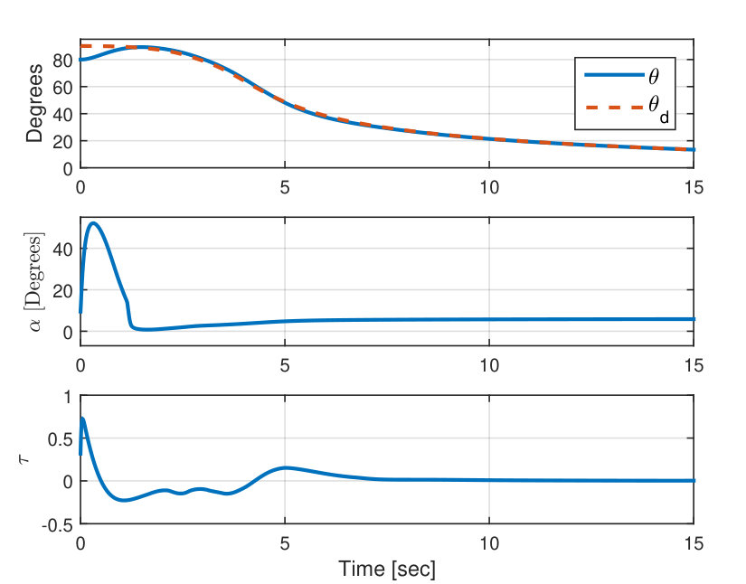 Figure 20
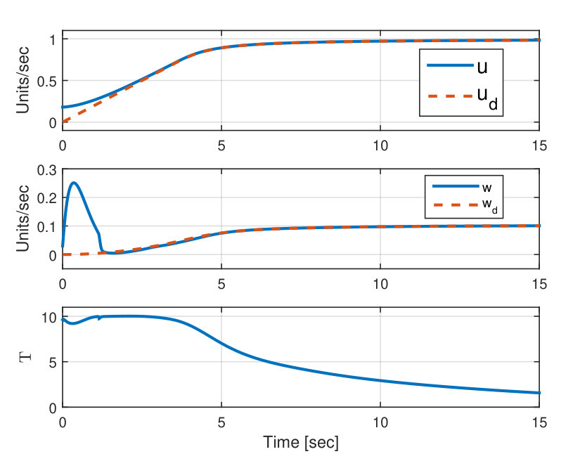 Figure 21
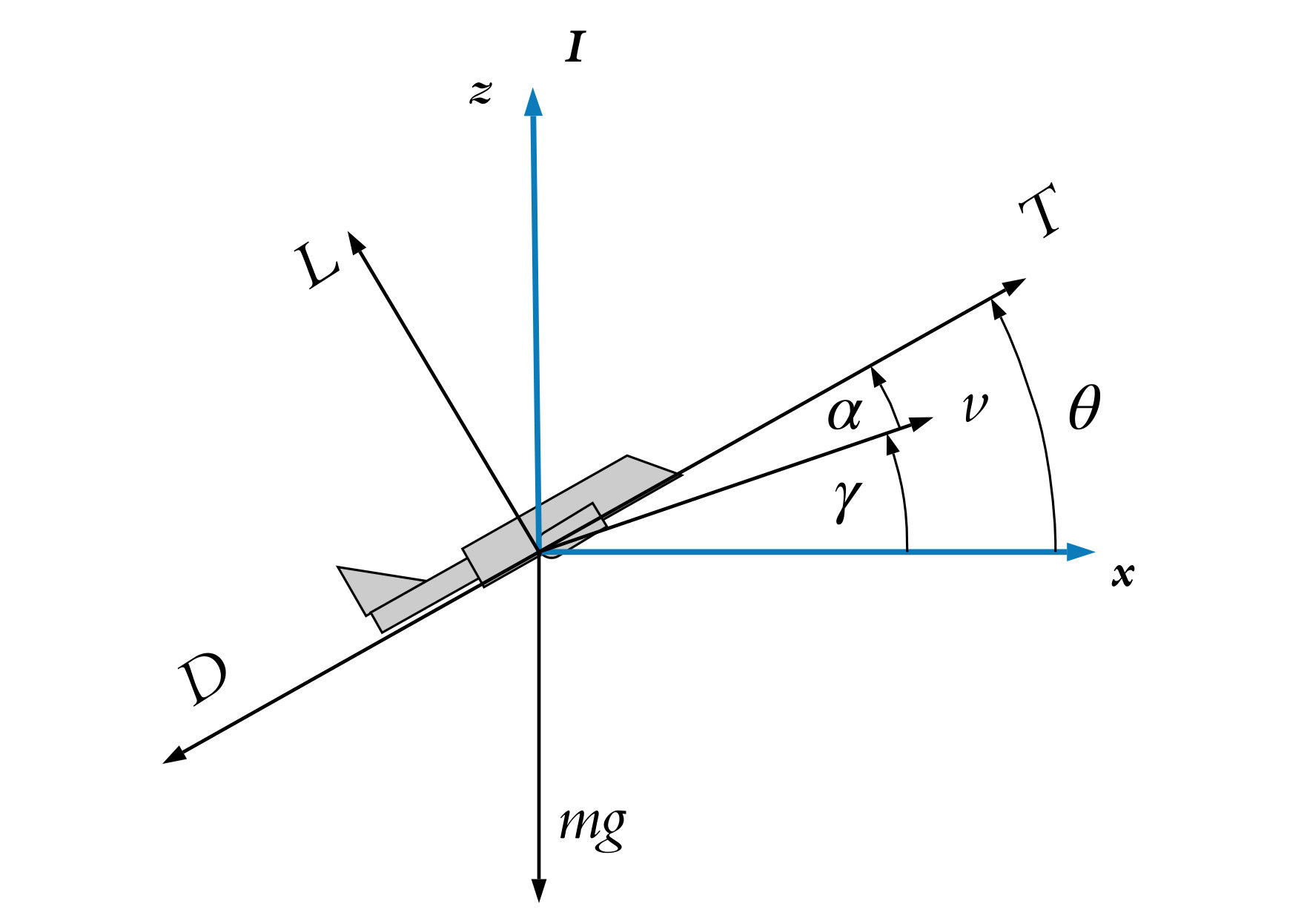 Figure 22
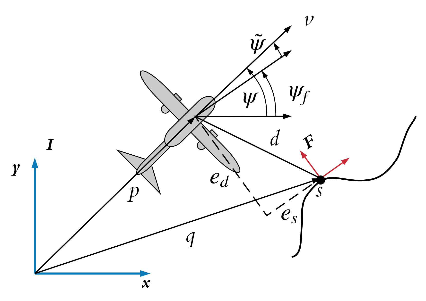 Figure 23
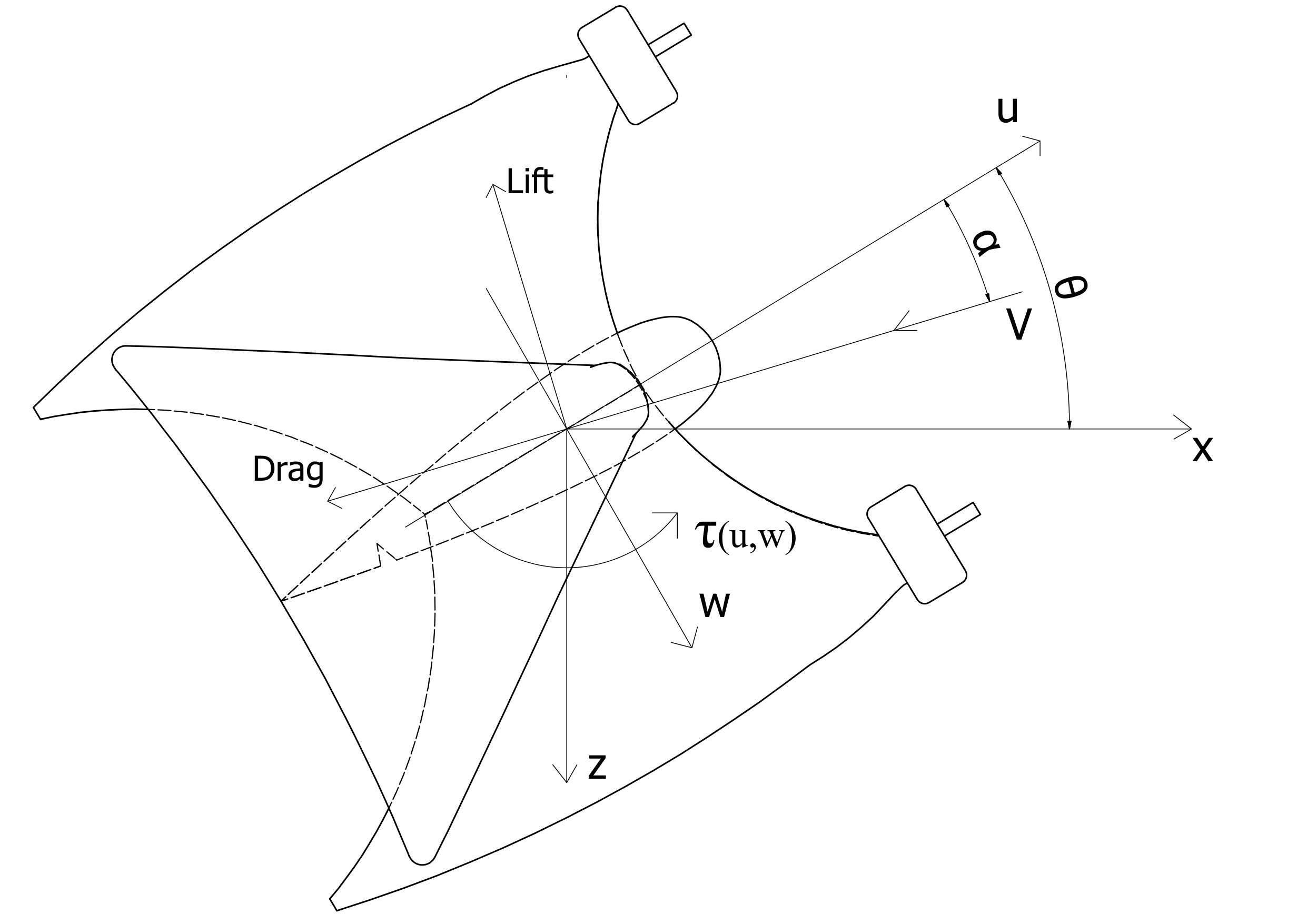 Figure 24
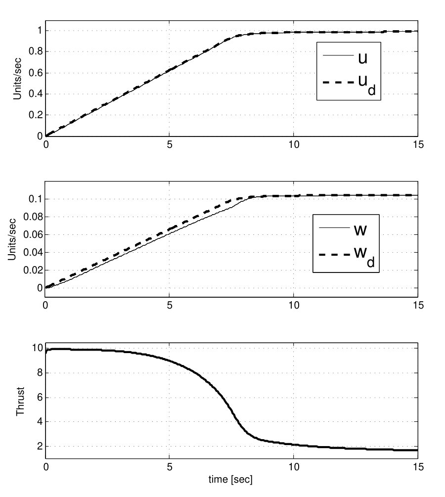 Figure 25
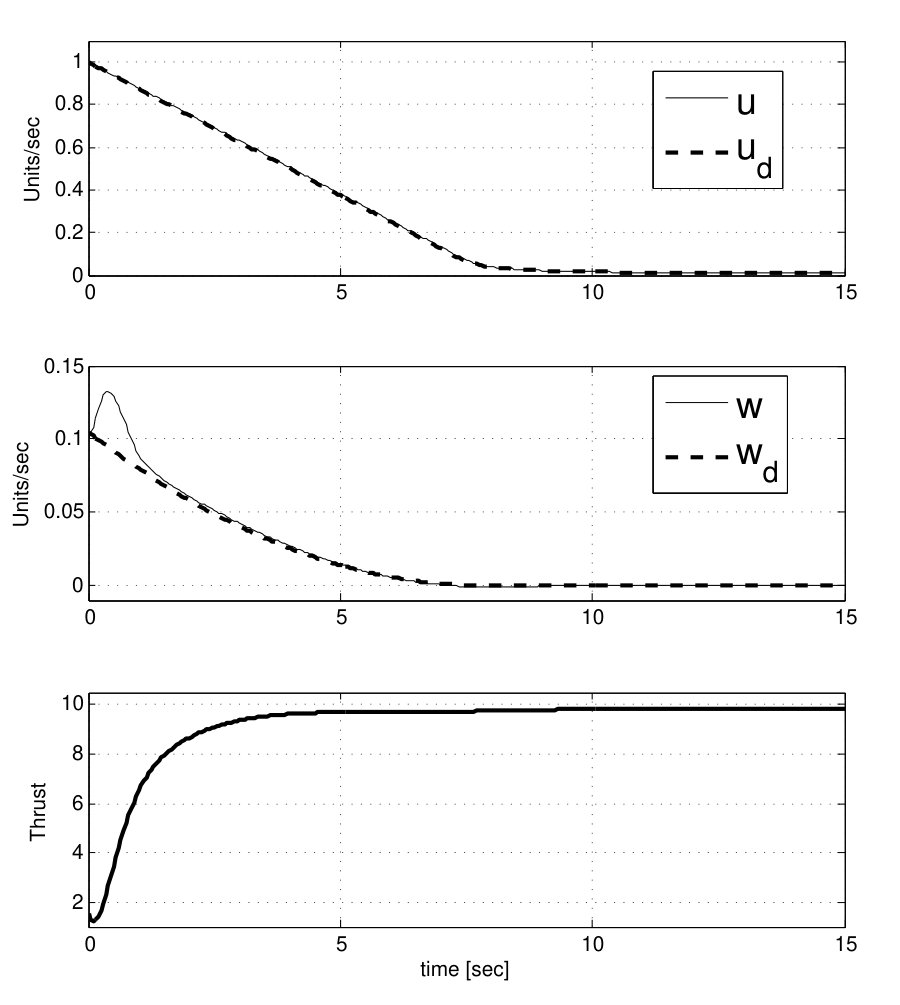 Figure 26
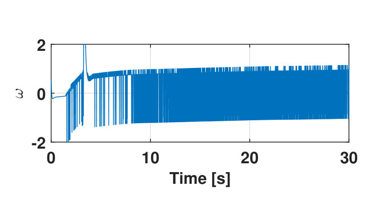 Figure 27
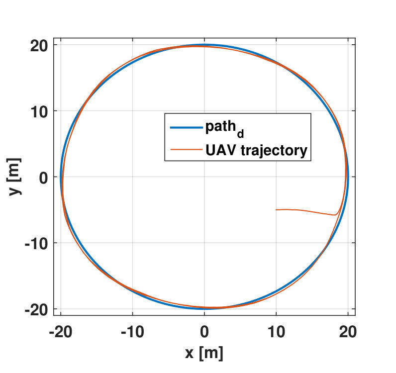 Figure 28
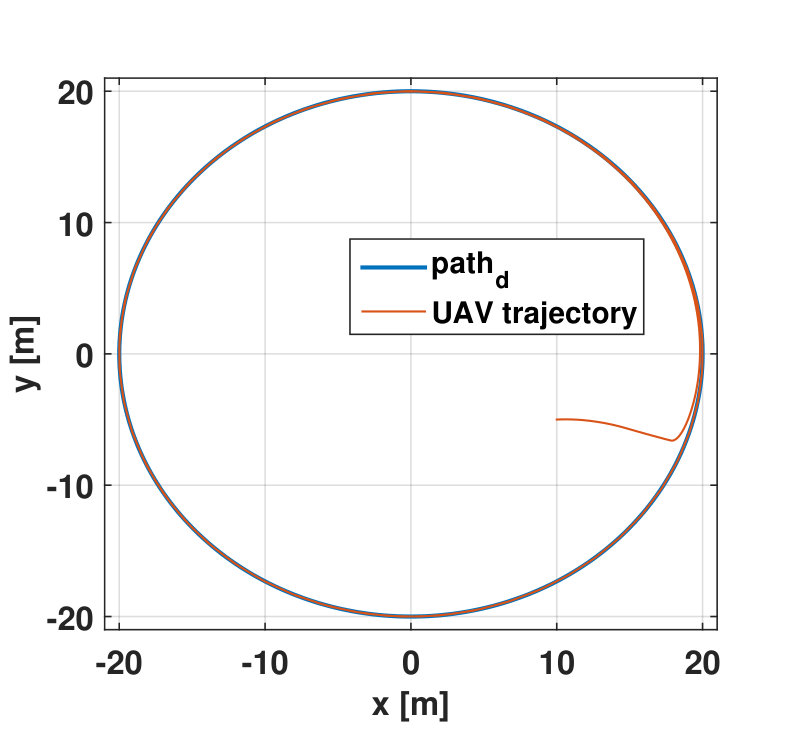 Figure 29
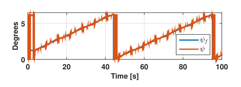 Figure 30
 Figure 31
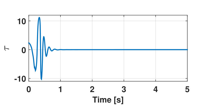 Figure 32
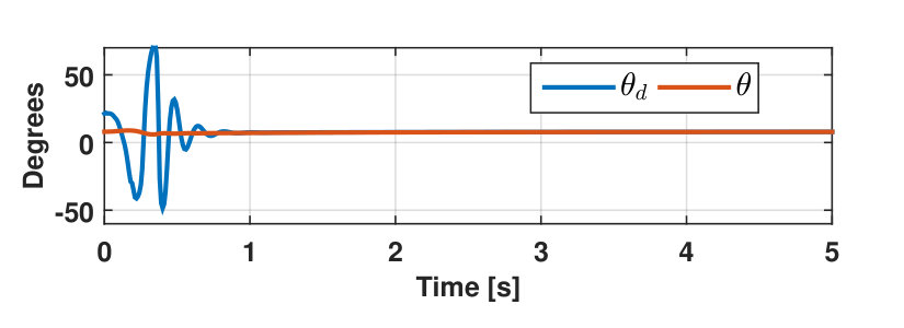 Figure 33
Peer Reviews
No public reviews on file for this paper yet. If you reviewed it on a platform where reviews are public (OpenReview, ICLR, NeurIPS, ICML), you can paste yours below so the community can read it here.
Videos
No videos yet. Explain this paper in a talk, walkthrough, or lecture? Add one.
Taxonomy
TopicsAdaptive Control of Nonlinear Systems · Aerospace Engineering and Control Systems · Guidance and Control Systems
A full controller for a fixed-wing UAV
Gerardo Flores, Alejandro Flores and Andrés Montes de Oca G. Flores, A. Flores and A. Montes de Oca are with the Perception and Robotics Laboratory, Centro de Investigaciones en Óptica, León, Guanajuato, Mexico, 37150. (email: [email protected], [email protected] and [email protected]). Corresponding author: Gerardo Flores.This work was supported partially by the FORDECYT-CONACYT under grant 292399 and by the Laboratorio Nacional de Óptica de la Visión of the CONACYT agreement 293411.
Abstract
This paper presents a nonlinear control law for the stabilization of a fixed-wing UAV. Such controller solves the path-following problem and the longitudinal control problem in a single control. Furthermore, the control design is performed considering aerodynamics and state information available in the commercial autopilots with the aim of an ease implementation. It is achieved that the closed-loop system is G.A.S. and robust to external disturbances. The difference among the available controllers in the literature is: 1) it depends on available states, hence it is not required extra sensors or observers; and 2) it is possible to achieve any desired airplane state with an ease of implementation, since its design is performed keeping in mind the capability of implementation in any commercial autopilot.
Index Terms:
Fixed-wing; path-following; UAV; longitudinal aircraft; dynamics Lyapunov-based control.
I Introduction
Fixed-wing Unmanned Aerial Vehicles (UAVs) have become relevant above the quadrotors in remote sensing applications, precision agriculture, and surveillance. This is due to its flight endurance, long flying times, high speeds and energy efficiency. Due to the inherent non-linearity condition of fixed-wing UAVs, effective control need to be applied to this type of vehicles so this is a topic that remains being a challenge. In this paper we propose a full controller that achieves to stabilize the airplane in a condition required to perform inspection and surveillance missions. Full control means that it can stabilize the UAV at any desired position and velocity taking into account the optimal angle of attack and aerodynamics. This controller is developed taking in mind its applicability in autopilots such as the popular Pixhawk.
I-A Literature review
In the vast majority of the works relating fixed-wing aircraft control, the problem is tackled based in three fundamental modeling-based cases: a) the longitudinal model where the airspeed, angle of attack and pitch dynamics are controlled; b) path-following in 2D and 3D, where desired and positions must be achieved respectively; and c) considering the full 6-DOF airplane mathematical model. Each of these approaches have its own pros and cons. Studying longitudinal model and path-following problem separately, inherits the problem of not considering the full control of the plane. Whereas in the path-following control the airspeed and aerodynamics are not considered, in the longitudinal approach the steering of the path is not taken into account. On the other hand, investigating the 6-DOF model-based control usually results in complex controls that includes a great quantity of parameters and terms that makes the implementation in real UAVs a complex task. Some of the most recent works of these three cases are shown at Table I.
Apart from the aforementioned approaches to control fixed-wing UAVs, there is the guidance law that resolves the problem of path following by a simple lateral acceleration command; this approach can be seen for instance in [19], and in the famous paper [20] which presents the guidance law implemented in the Pixhawk commercial autopilot.
Regarding control techniques used for solving the control problem there are for instance: backstepping [21], [22], [23]; gain scheduled [24]; sliding mode [25]; model referenced adaptive control [26]; model predictive control [27], [28]; active disturbance rejection control [29]; among others.
I-B Contribution
The motivation to develop this work is twofold: a) present an algorithm that fully controls the fixed-wing UAV considering aerodynamics and the path steering problem; and b) design a controller as simple as possible that effectively stabilizes the system in the complete flight dynamics, i.e. stabilizing aircraft position, angle of attack, pitch dynamics, flight-path angle, yaw dynamics and airspeed (and as a consequence dynamics) to some given desired states. The controlled is designed having in mind its implementation in the Pixhawk autopilot using the sensor information available on it.
I-C Paper structure
The rest of the paper is structured as follows. In Section II the fixed-wing mathematical model is described, then based on desired states an error model is obtained. Section III presents the full control that stabilized the complete system, a formal proof is given. Section IV contains the simulation results that validates the effectiveness of the control. Finally, in Section V some comments and future work are presented.
II Problem Formulation
II-A System Model
Consider the following mathematical model representing the longitudinal and lateral dynamics according to Fig. 1.
[TABLE]
where is the airspeed of the drone, , and are the angle of attack (AoA), the bank and the pitch angle, respectively, and are the drag and lift forces generated by the aerodynamics of the wing, and are the velocities in the inertial frame (), and is the yaw angle. As control inputs, the dynamics can be controlled by , and . Without loss of generality, let normalize system (5), i.e. and then it is rewritten as
[TABLE]
We need to introduce the error of the angles. So, first, we define the velocity, bank angle and pitch errors as
[TABLE]
Using (18) in (14) and considering that , then we have
[TABLE]
If we define the following coordinate change
[TABLE]
and consider that . The system changes to
[TABLE]
where .
For the lateral model, we define orientation and position errors according to Fig. 1(a). This path following approach has been investigated in our previous work [4] where a virtual particle that moves over the desired path according to the velocity and heading of the UAV is used to achieve the following task. So, the errors are defined as follows [4]
[TABLE]
where and are the and the errors, respectively, between the virtual particle and the position of the UAV in the inertial frame that is expressed in the velocity particle frame . This rotation angle is the defined as
[TABLE]
It is also introduced the path curvature of the desired trajectory as . As , the previous system now is
[TABLE]
Gathering (23) and (27), the complete error model is given by
[TABLE]
III Main Result
In this section the main result is resented. For that, let consider the following assumptions.
Assumption 1
The airspeed velocity is always positive, i.e. with .
Assumption 2
* and are considerd constants.*
Assumption 3
The initial airspeed is positive, i.e., the fixed-wing UAV has taken off and is flying in the air.
The main results is presented in the next
Theorem 1
Let system (35) under controls (46), (49), (58) and (61) then the closed loop system is globally asymptotically stable.
Proof:
The goal is to get and with . It is important to highlight that the algebraic equation must be always fulfilled. This is a condition inherent of the AoA, pitch and flight-path angle. Let consider the following function
[TABLE]
where
[TABLE]
with . The time derivative of is
[TABLE]
where we have designed the control term as
[TABLE]
and then under this control the time derivative of results in
[TABLE]
Now obtaining the time derivative of we obtain
[TABLE]
where we choose the control term equal to
[TABLE]
and therefore
[TABLE]
Considering and as temporal control inputs, we can extract as
[TABLE]
is obtained from obtaining as follows
[TABLE]
this is the commanded for . The pitch error subsystem can be represented by
[TABLE]
Let
[TABLE]
then where It follows that
[TABLE]
with the Lyapunov equation with . Then, it follows that the time derivative of (36) is given by
[TABLE]
From the previous analysis one concludes that all trajectories are bounded, i.e. for each trajectory there is an such that .
It is known that any bounded trajectory of an autonomous system like (35), converges to an invariant set [30]. Let such system invariant set be . By construction we can say that
[TABLE]
where is a Lyapunov function for (35). Let find by combining , which is not dependent of every states in (35), with the positive definite function
[TABLE]
where
[TABLE]
where is a function which is saturated as in [31] that satisfies the condition . Let’s compute the time derivative of and then we get
[TABLE]
If we define as
[TABLE]
then
[TABLE]
Now if we obtain the time derivative of
[TABLE]
then consider the following proposed control
[TABLE]
then
[TABLE]
Using (60) and (63) in (56), it follows that
[TABLE]
Then, as
[TABLE]
[TABLE]
From (54) it follows that
[TABLE]
Then if we define from (69) as
[TABLE]
and we substitute (73) and (71) in (69) we have
[TABLE]
and
[TABLE]
since , then if . Also, if and the remaining states are zero, . Then it is clear that and in . Let the set of all points where given by
[TABLE]
Note that the rest of is equal to zero at zero. Observing the closed loop system (35) with the controls (46), (49) and (61) when and one obtains
[TABLE]
then is the only solution of (78) and therefore the largest invariant set in is the origin and by the LaSalle invariance principle as ; as long as the initial state be in . And the closed loop system is asymptotically stable in the arbitrary large set: provided that . Also as , i.e. is radially unbounded, then the closed loop system is G.A.S. ∎
IV Simulation Experiments
To verify the stability in a computational environment, a numerical simulation of the systems (5) and (9) under controls (46), (49), (58) and (61) is performed. The parameters used in the simulation are: , , , , , , , , , , , , where is a constant that describes the air density an the area of the wind. The initial conditions for the simulation are: , , , , , , . The induced disturbance to the state is a sinusoidal signal with units of amplitude and a frequency of . The airspeed is depicted at Fig. 2. The control applied to the model is shown in Fig. 3.
Another important fact that determines an optimal flight of the UAV is the AoA. According to the lift coefficient of the wing profile used for this simulation, which is a symmetric profile, the best AoA in relation with the lift-drag coefficients is around . Then, it is expected that this angle is reached during stabilization process. This AoA and the other aerodynamic terms have been taken from the UAV presented in our previous work [32]. In Fig. 4 it is shown the angles evolution including the AoA convergence to the desired value equal to .
The control input is shown at Fig. 5. With this control it is possible to reach the according to and .
In Fig.6, the control is plotted. With this control, is guided to the desired heading for the path following.
Finally, Figs. 7 and 8 depict the UAV’s position w.r.t. the desired path, which is in this case a circle of radius with and without disturbance in , respectively.
V Conclusions
We have presented a full controller for a fixed-wing UAV which presents robust capabilities for disturbances presented in the UAV dynamics. A stability proof is presented which demonstrated that the closed-loop system is GAS.
As future work we intend to implement this controller used the approach known as hardware in the loop (HIL) and finally be implemented in the real fixed-wing UAV in a Pixhawk autopilot.
The reference list from the paper itself. Each links out to its DOI / PubMed record.
- 1[1] Y. Hamada, T. Tsukamoto, and S. Ishimoto, “Receding horizon guidance of a small unmanned aerial vehicle for planar reference path following,” Aerospace Science and Technology , vol. 77, pp. 129–137, June 2018.
- 2[2] S. Zhao, X. Wang, Z. Lin, D. Zhang, and L. Shen, “Integrating Vector Field Approach and Input-to-State Stability Curved Path Following for Unmanned Aerial Vehicles,” IEEE Transactions on Systems, Man, and Cybernetics: Systems , pp. 1–8, 2018.
- 3[3] R. P. Jain, A. P. Aguiar, and J. Sousa, “Self-triggered cooperative path following control of fixed wing Unmanned Aerial Vehicles,” in 2017 International Conference on Unmanned Aircraft Systems (ICUAS) . Miami, FL, USA: IEEE, June 2017, pp. 1231–1240.
- 4[4] G. Flores, I. Lugo-Cárdenas, and R. Lozano, “A nonlinear path-following strategy for a fixed-wing mav,” in 2013 International Conference on Unmanned Aircraft Systems (ICUAS) , May 2013, pp. 1014–1021.
- 5[5] I. Kaminer, A. Pascoal, E. Xargay, N. Hovakimyan, C. Cao, and V. Dobrokhodov, “Path Following for Small Unmanned Aerial Vehicles Using L 1 Adaptive Augmentation of Commercial Autopilots,” Journal of Guidance, Control, and Dynamics , vol. 33, no. 2, pp. 550–564, Mar. 2010.
- 6[6] G. Vanegas, F. Samaniego, V. Girbes, L. Armesto, and S. Garcia-Nieto, “Smooth 3d path planning for non-holonomic UA Vs,” in 2018 7th International Conference on Systems and Control (ICSC) . Valencia: IEEE, Oct. 2018, pp. 1–6.
- 7[7] T. Oliveira, A. P. Aguiar, and P. Encarnacao, “Three dimensional moving path following for fixed-wing unmanned aerial vehicles,” in 2017 IEEE International Conference on Robotics and Automation (ICRA) . Singapore, Singapore: IEEE, May 2017, pp. 2710–2716.
- 8[8] N. Cho, Y. Kim, and S. Park, “Three-Dimensional Nonlinear Differential Geometric Path-Following Guidance Law,” Journal of Guidance, Control, and Dynamics , vol. 38, no. 12, pp. 2366–2385, Dec. 2015.