On the convergence of the maximum likelihood estimator for the transition rate under a 2-state symmetric model
Lam Si Tung Ho, Vu Dinh, Frederick A. Matsen IV, Marc A. Suchard

TL;DR
This paper proves that the maximum likelihood estimator for the transition rate in a 2-state symmetric trait evolution model converges to the true value as the number of species increases, under certain regularity conditions.
Contribution
It establishes the convergence and provides bounds for the MLE of the transition rate in a large-tree limit for a 2-state symmetric model, extending previous results to correlated trait data.
Findings
MLE converges to the true transition rate under regularity conditions
Provides an upper bound for the estimation error
Results apply to various practical tree models such as Yule and coalescent trees
Abstract
Maximum likelihood estimators are used extensively to estimate unknown parameters of stochastic trait evolution models on phylogenetic trees. Although the MLE has been proven to converge to the true value in the independent-sample case, we cannot appeal to this result because trait values of different species are correlated due to shared evolutionary history. In this paper, we consider a -state symmetric model for a single binary trait and investigate the theoretical properties of the MLE for the transition rate in the large-tree limit. Here, the large-tree limit is a theoretical scenario where the number of taxa increases to infinity and we can observe the trait values for all species. Specifically, we prove that the MLE converges to the true value under some regularity conditions. These conditions ensure that the tree shape is not too irregular, and holds for many practical…
Click any figure to enlarge with its caption.
 Figure 1
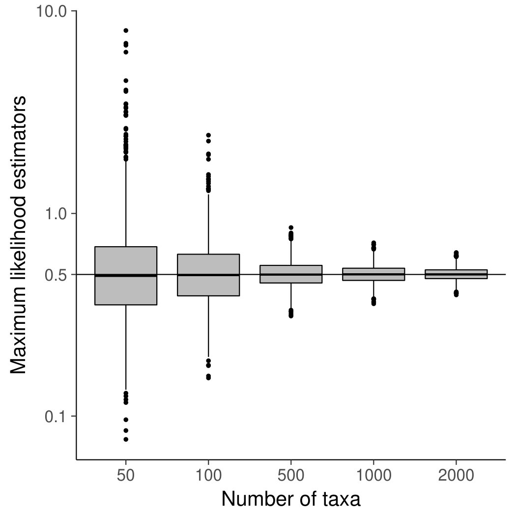 Figure 2
Peer Reviews
No public reviews on file for this paper yet. If you reviewed it on a platform where reviews are public (OpenReview, ICLR, NeurIPS, ICML), you can paste yours below so the community can read it here.
Videos
No videos yet. Explain this paper in a talk, walkthrough, or lecture? Add one.
On the convergence of the maximum likelihood estimator for the transition rate under a -state symmetric model
Lam Si Tung Ho
Department of Mathematics and Statistics
Dalhousie University, Halifax, Nova Scotia, Canada These authors contributed equally to this work.
Vu Dinh*∗*
Department of Mathematical Sciences
University of Delaware
Frederick A. Matsen IV
Program in Computational Biology
Fred Hutchinson Cancer Research Center
Marc A. Suchard
Departments of Biomathematics, Biostatistics and Human Genetics
University of California, Los Angeles
Abstract
Maximum likelihood estimators are used extensively to estimate unknown parameters of stochastic trait evolution models on phylogenetic trees. Although the MLE has been proven to converge to the true value in the independent-sample case, we cannot appeal to this result because trait values of different species are correlated due to shared evolutionary history. In this paper, we consider a -state symmetric model for a single binary trait and investigate the theoretical properties of the MLE for the transition rate in the large-tree limit. Here, the large-tree limit is a theoretical scenario where the number of taxa increases to infinity and we can observe the trait values for all species. Specifically, we prove that the MLE converges to the true value under some regularity conditions. These conditions ensure that the tree shape is not too irregular, and holds for many practical scenarios such as trees with bounded edges, trees generated from the Yule (pure birth) process, and trees generated from the coalescent point process. Our result also provides an upper bound for the distance between the MLE and the true value.
1 Introduction
The maximum likelihood estimator (MLE) is frequently used to estimate unknown parameters in trait evolution models on phylogenetic trees. To safely use this machinery, it is important to know that the MLE is consistent: that is, the estimate converges to the true value as we observe trait values for more species. However, traditional statistical theory only guarantees the consistency of the MLE when observations are independent and identically distributed. In contrast, trait values of biological species are not independent because species are related to each other according to a phylogenetic tree. Therefore, traditional consistency results are not directly applicable to trait evolution studies. For this paper we consider the scenario where only a single trait is observed and the number of species increases to infinity. This is different from the setting where many traits/characters are observed for the same set of species; this alternate setting typically assumes independence between traits.
Binary traits studied by comparative biologists come in various types, including morphological traits (whether a fruit fly has curly wings), behavioral traits (whether an antelope hides from predators), and geographical traits (whether a species is aquatic). Here we study the consistency property of the MLE for estimating the transition rate of a binary trait evolved along a phylogenetic tree according to a -state symmetric Markov process. Under this -state symmetric model, there is an unique rate of switching back and forth between the two states of a phenotype, which is the parameter of interest. We show that under two mild conditions, the MLE of this transition rate is consistent, that is, the estimate converges to the correct value as we observe the trait values of more species. These conditions ensure that edge lengths of the tree are not too small and the pairwise distances between leaves are neither too small nor too large. We verify that these conditions holds for many practical cases including trees with bounded edges, trees generated from the Yule process (Yule, 1925), and trees generated from the coalescent point process (Lambert and Stadler, 2013).
The consistency of the MLE does not always hold under trait evolution models. Indeed, for estimating the ancestral state of the -state symmetric model, Li et al. (2008) point out that the MLE can be inconsistent. As a consequence, the estimate of the ancestral state may not be close to the true value no matter how many species have been sampled. Several efforts have also been made to investigate the consistency of the MLE under evolution models of a continuous trait. Ané (2008) points out that unlike traditional linear regression, the MLE of the coefficients of phylogenetic linear regression under the Brownian motion model can be inconsistent. Additionally, Sagitov and Bartoszek (2012) show that the sample mean is an inconsistent estimator for the ancestral state under this model when the tree is generated from the Yule process. For the Ornstein-Uhlenbeck model, Ho and Ané (2013) show that if the height of the phylogenetic tree is bounded as more observations are collected, then the MLE of the selective optimum is not consistent. Moreover, they discovered that in this scenario, no consistent estimator for the selective optimum exists. Recently, Ané et al. (2017) provide a necessary and sufficient condition for consistency of the MLE under the Ornstein-Uhlenbeck model. Although the problem of reconstructing the ancestral state under the -state symmetric model has been studied extensively (Tuffley and Steel, 1997; Mooers and Schluter, 1999; Li et al., 2008; Mossel and Steel, 2014), it remains unknown whether the transition rate can be estimated consistently.
In this paper, we show that the MLE is a consistent estimator for the transition rate of the -state symmetric model under simple conditions. We start with introducing the -state symmetric model for binary traits and derive several statistical properties of this model in Section 2. In Section 3, we state two necessary conditions for the consistency of the MLE of the transition rate and provide a detailed proof for this result. Section 4 verifies these conditions for several practical scenarios and illustrates our result through a simulation.
2 Properties of the -state symmetric model
Let be the transition rate of a -state symmetric Markov process. Then, the transition probability matrix has an analytical form:
[TABLE]
Hence, the probability that the process switches state after unit of time is .
In this paper, the term phylogenetic tree (or phylogeny) refers to a bifurcating rooted tree with leaves labeled by a set of taxon (species) names. We can reroot a phylogenetic tree by moving the root to another location along the tree (see Figure 1). The evolution of a binary trait along a tree is modeled using the -state symmetric Markov process as follows. At each node in the phylogeny, the children inherit the trait value of their parent and the trait of each child evolves independently of one another.
Let be a phylogenetic tree with leaves, and be the trait values at the leaves of . We assume that the ancestral state at the root of follows a stationary distribution, which is a Bernoulli distribution with success probability . Let be the set of all edges of . The joint probability distribution of is
[TABLE]
where ranges over all extensions of to the internal nodes of the tree, denotes the assigned state of node by , is the edge length of , and is the element at -th row and -th column of matrix . We define the log-likelihood function as . Throughout this paper, we denote the true transition rate with and assume that where are two known positive numbers. Define
[TABLE]
Then the Kullback-Leibler divergence from to is
[TABLE]
where is the expectation with respect to .
Lemma 1**.**
Let be the phylogenetic tree obtained by rerooting a tree , then
[TABLE]
for any trait values at the leaves.
This lemma, sometimes called the “pulley principle,” is a direct consequence of the fact that the ancestral state follows a stationary distribution (Felsenstein, 1981). We also have the following Lemmas:
Lemma 2**.**
Let be a rooted tree with root , and be the trait values at the leaves of generated under the -state symmetric model. Let be a function such that , where denotes the all-ones vector. Then, and the trait value at are independent.
The following two lemmas concern the regularity of the log-likelihood function. In particular, Lemma 3 shows that the log-likelihood function of a binary tree can be bounded by the sum of the log-likelihood functions of its two subtrees.
Lemma 3**.**
Let and be two direct descendants of , and and the two subtrees descending from them. Let , be the observations at the leaves of and . We have
[TABLE]
where is the tree distance between and .
Lemma 4** (Uniform Lipschitz).**
There exists such that
[TABLE]
where denotes the number of leaves of .
The proofs of Lemmas 2, 3, and 4 are provided in the Appendix A. Henceforth we will also use to denote the trait value at the root by an abuse of notation.
3 Convergence of the MLE of the transition rate
The MLE of is defined as follows:
[TABLE]
In this section, we will state our main result regarding the consistency of . We will need to make two assumptions to ensure that the shape of is not too irregular. Let us define
[TABLE]
where denotes the edge length of edge .
Assumption 1**.**
) for some . That is, there exists a universal constant such that .
Assumption 2**.**
There exist pairs of leaves such that the paths connecting each pair are pairwise disconnected and their lengths are bounded in some fixed range . Here, denotes a quantity that is greater than for a positive constant and all .
Assumption 1 makes sure that the edge lengths of are not too small. It is worth noticing that when is small enough. Therefore, this assumption holds when the smallest edge length is . On the other hand, Assumption 2 guarantees that the pairwise distances between leaves of do not vary too extremely. In Section 4, we will verify these assumptions for several common tree models. Although we employ rerooting in proofs below, Assumption 1 is for the original root of the tree.
Theorem 1**.**
Under Assumptions 1 and 2, for any , , there exists a constant such that
[TABLE]
with probability .
From now on, we will use and as short for and . Recall that is the log-likelihood function and where is the true value of the transition rate. The main ideas of the proof of Theorem 1 can be outlined as follows. For a fixed value of , we can view the function as the evidence to distinguish between and . We will prove that as the number of leaves approaches infinity, the information to distinguish and , characterized by the KL divergence between to (which is equal to ) increases linearly (Lemma 6), while the associated uncertainty, characterized by the variance of , only increases sub-quadratically (Lemma 9). It is worth noting that while the results of Lemma 6 and Lemma 9 are straightforward for independent and identically distributed data, the analyses for phylogenetic traits are more complicated due to the correlations between trait values at the leaves. To overcome this issue, we use the independent phylogenetic contrasts, introduced in the next section, to obtain a lower bound on the information. On the other hand, Lemma 3 shows that the log-likelihood function of a binary tree can be bounded by the sum of the log-likelihood functions of its two subtrees, which allows us to exploit the sparse structure of the tree to derive an upper bound on uncertainty through an induction argument. Finally, we obtain a uniform bound on the difference between the log-likelihood functions and its expected values (Lemma 10), which enables us to derive an analysis of convergence of the MLE.
3.1 Lower bound on information
Phylogenetic contrasts
Letting and be two different species, we define to be a contrast between the two species. This is a popular notion introduced by Felsenstein (1985) for computing the likelihood function under the Brownian motion model. Ané et al. (2017) use independent contrasts to construct consistent estimators for the covariance parameters of the Ornstein-Uhlenbeck model. Here, we will introduce a notion of a squared-contrast , which is simply the square of a contrast , and show that squared-contrasts have the same independence properties as independent contrasts. Let be the state of the most recent common ancestor of and , the tree distance from to , and the path on the tree connecting and . By symmetry of the model, we have
[TABLE]
Therefore, and are independent.
Lemma 5** (Sequence of contrasts).**
Let be a sequence of contrasts such that any two paths in have no common node. Then are independent.
Proof.
We have, using here to denote expectation over ancestral states,
[TABLE]
where the third equality comes from the Markov property. This completes the proof. ∎
The independent squared-contrasts allow us to derive the following lower bound on the information.
Lemma 6**.**
Under Assumption 2, there exists such that
[TABLE]
for all .
Proof.
Under Assumption 2, there exists a set of pairwise disjoint pairs (that is, the paths connecting each pair are pairwise disconnected) . Consider the corresponding set of squared-contrasts . By Lemma 5, are independent. Let be the distribution of corresponding to parameter . The total variation from to is
[TABLE]
By the data processing inequality (Theorem 9 in Van Erven and Harremoës, 2014), the fact that are independent, and Pinsker’s inequalities, we have
[TABLE]
Note that which completes the proof. ∎
3.2 Upper bound on the uncertainty
The result of Section 3.1 indicates that as the number of leaves increases, the information to distinguish and also increases linearly. In order to prove that the MLE can successfully reconstruct the true parameter , we need to ensure that such information is not confounded by the uncertainty associated with the log-likelihood function due to randomness in the data. In other words, we want to guarantee that as , the variance of only grows sub-quadratically, that is, there exist and such that . To obtain the bound, we need the following Lemma, the proof of which appears in Appendix A.
Lemma 7**.**
If two functions and satisfy , then for all and random variables ,
[TABLE]
Recalling that,
[TABLE]
we have the following estimate that does not depend on Assumption 1.
Lemma 8**.**
For all and , there exist such that
[TABLE]
for all trees with taxa and .
Proof.
We will prove the result by induction in the number of taxa . For , we apply Lemma 4 to obtain
[TABLE]
where is the constant in Lemma 4. Thus . Assume that the statement is valid for all . We will prove that it is also valid for . Now, let be a bifurcating tree with taxa. Lipton and Tarjan (1979) show that there exists an edge of such that if we reroot at the middle of this edge, the two subtrees and stemming from and have no more than leaves. Let be the middle point of edge and be the tree obtained by rerooting to . Denote by and the number of leaves of and . According to Lemma 1 and Lemma 2,
[TABLE]
By Lemma 3, we have . We apply Lemma 7 to obtain
[TABLE]
Let and be the observations at the leaves of and respectively. Since and are independent conditional on , we have . By Lemma 2, we deduce that
[TABLE]
Recalling that the trees and have no more than leaves, using the induction hypothesis for and , we have
[TABLE]
Let and be the edges stemming from the root of . By definition, we have
[TABLE]
where the last inequality comes from the fact that is a non-increasing function. Thus, if we choose such that
[TABLE]
then
[TABLE]
which completes the proof. ∎
A combination of Lemma 8 and Assumption 1 gives rise to the desired bound:
Lemma 9** (Sub-quadratic upper bound on variance).**
Under Assumption 1, , there exists such that
[TABLE]
for all and .
Proof.
By Lemma 8 and Assumption 1, we have
[TABLE]
Note that . So, , we can choose . ∎
3.3 Concentration bound
We are now ready to prove the concentration inequality for the 2-state symmetric model.
Lemma 10** (Concentration bound).**
Under Assumption 1, for any and , there exists such that
[TABLE]
with probability at least .
Proof.
Applying Chebyshev’s inequality, we obtain
[TABLE]
for any . On the other hand, by Lemma 4, we have
[TABLE]
Therefore, if
[TABLE]
then
[TABLE]
for all
[TABLE]
Define
[TABLE]
We have
[TABLE]
The last inequality comes from Lemma 9. We complete the proof by picking
[TABLE]
∎
3.4 Proof of Theorem 1
From Lemma 6, we have
[TABLE]
where is the expectation with respect to .
Note that
[TABLE]
By Lemma 10, with probability , we obtain
[TABLE]
which completes the proof.
4 Applications
In this section, we discuss applications of Theorem 1 for several practical scenarios. We first consider trees with edges of bounded length.
Theorem 2** (Trees with bounded edges).**
If edge lengths of are bounded from below and above, then the MLE is consistent.
Proof.
Since all edge lengths are bounded from below, Assumption 1 holds with . Next, we will show that Assumption 2 is satisfied. We select pairs of leaves using the following procedure:
Pick a cherry as a pair. 2. 2.
Remove the cherry from the tree as well as the edge immediately above it. 3. 3.
Repeat step 1 and 2 until the tree has [math] or leaves.
Denote be the set of pairs returned by the procedure where . It is obvious that the paths connecting each pair are pairwise disjoint. Let and be the lower and upper bound of edge lengths, so we have a lower bound for distances between each pair . Moreover,
[TABLE]
We will prove by contradiction that the set has at least elements. Assume that . Note that
[TABLE]
We deduce that
[TABLE]
Therefore
[TABLE]
which contradicts (3). Therefore, .
∎
Next, we apply our result to trees generated from a pure-birth process (Yule, 1925). This is a classical tree-generating process which assumes that lineages give birth independently to one another with the same birth rate.
Theorem 3** (Yule process).**
If is generated from a Yule process, then the MLE is consistent.
Proof.
Again, we only need to check Assumptions 1 and 2. Let be the amount of time during which has lineages. Then, are independent exponential random variables with rate where is the birth rate of the Yule process. Let be the minimum edge length of . It is sufficient for us to show that . Indeed, we have
[TABLE]
which converges to as . Hence, Assumption 1 is satisfied asymptotically with .
Define the age of an internal node to be its distance to the leaves. By Corollary 4 of Ané et al. (2017), there exist such that the probability of there being internal nodes with age between and is . Let be the set of internal nodes which have age between and , we select pairs of leaves as follows:
Start with an internal node that has the smallest age. Pick two of its descendants such that is their most recent common ancestor to form a pair. 2. 2.
Remove and its parent node from . 3. 3.
Repeat step 1 and 2 until is empty.
This procedure is similar to the procedure for selecting contrasts in Ané et al. (2017, Lemma 3). Hence, it selects at least pairs, which is of order . Since these internal nodes have age between and , Assumption 2 is satisfied.
∎
Finally, we consider the coalescent point process (CPP), which generates a random ultrametric tree with a given height (see Lambert and Stadler, 2013, for more details). Conditioning on the number of species , the internal node ages of the tree generated from the CPP are independent and identically distributed according to a probability distribution in . The probability density function of this common distribution is called the coalescent density. We say that a CPP is regular if its common distribution is not a point mass at [math] and the coalescent density is bounded from above.
Theorem 4** (Coalescent point process).**
If is generated from a regular coalescent point process, then the MLE is consistent.
Proof.
Denote the minimum edge length of by . We have
[TABLE]
Therefore,
[TABLE]
By the results of Section 4 in Jammalamadaka and Janson (1986) (for which the details will be provided in the Appendix), we have
[TABLE]
for any . We deduce that
[TABLE]
Since can be arbitrary small, we conclude
[TABLE]
On the other hand
[TABLE]
Note that is bounded from above by in , thus
[TABLE]
where is the upper bound of . Hence,
[TABLE]
Similarly,
[TABLE]
Therefore,
[TABLE]
Hence, Assumption 1 is satisfied.
Since the common distribution is not a point mass at [math], there exist a constant such that . Let be the set of internal nodes of which have age between and . Then, Assumption 2 holds if we can prove that is of order because we can use the same argument as in the proof of Theorem 3. By strong law of large numbers, we have
[TABLE]
which completes the proof.
∎
5 Practical implication
The consistency property proved in Theorem 1 suggests that adding more taxa helps to significantly improve the accuracy of the MLE of the transition rate. It is worth noticing that this property does not hold in many scenarios (see Li et al., 2008; Ané, 2008; Ho and Ané, 2013, 2014). To illustrate our theoretical results, we perform the following simulation using the R package geiger (Harmon et al., 2007; Pennell et al., 2014). We simulate trees (the number of taxa varies from to ) according to the Yule process with birth rate . For each tree, we simulate traits under the -state symmetric model with the transition rate . For each of these 100 traits, the MLE for the transition rate is computed separately. The result is summarized in Figure 2. We can see that the MLEs concentrate more and more around the true transition rate as the number of species increases.
6 Discussion
In this paper, we investigate the convergence of the MLE for the transition rate of a -state symmetric model under regularity conditions on tree shape. These conditions ensure that edge lengths of the tree are not too small and the pairwise distances between leaves are not too extreme. For example, these conditions are satisfied when the edge lengths of the tree are bounded from above and below. We have also verified that trees generated from pure-birth process and coalescent point process satisfy these conditions. On the other hand, whether these sufficient conditions are also necessary conditions remains open.
Our results suggest that adding data in terms of the number of tips tends to improve the accuracy of the MLE of the transition rate in general. To demonstrate this result, we use simulations to confirm that the MLE of the transition rate is consistent when the tree is generated from the Yule process. It is worth noticing that for evolutionary data, the MLE for other quantities of interest in evolutionary studies can be inconsistent (Li et al., 2008; Ané, 2008; Ho and Ané, 2013, 2014). In these situations, adding more data is a waste of resources because it does not significantly improve the precision of the MLE. Therefore, it is important to study the consistency of the MLE in the context of trait evolution models.
Beside its practical biological application, the paper also investigates many theoretical properties of tree-generating processes. Specifically, in Theorem 3 and Theorem 4, we consider the problem of bounding the minimum edge length of a tree generated by Yule and coalescent point processes. The theorems show that generically, is bounded from below by a function of order for the Yule process and for the coalescent point process. Since the minimum edge length plays an important role in many phylogenetic problems, these results may be of independent interest.
Finally, we remark that if we have multiple independent traits which evolve according to the same 2-state Markov process, the distance from the MLE to the true value of the transition rate will decrease linearly with respect to the number of traits. This result comes from the fact that traditional properties of MLE can be applied because these traits are independent. Therefore, incorporating additional traits to the analysis is another way to improve the precision of the MLE.
Appendix A Proofs
A.1 Proof of lemma 2
Note that by symmetry, we have . We deduce that
[TABLE]
which completes the proof.
A.2 Proof of lemma 3
Denote for , . We have
[TABLE]
Moreover
[TABLE]
Therefore
[TABLE]
A.3 Proof of lemma 4
Without loss of generality, we assume that . By the mean value theorem, there exists for any such that
[TABLE]
We observe that there exists a such that
[TABLE]
Therefore,
[TABLE]
This implies that
[TABLE]
Note that
[TABLE]
By applying (5) for all edges on the tree, we deduce that
[TABLE]
Hence,
[TABLE]
which validates the lemma.
A.4 Proof of lemma 7
For all , we have . Let be an independent and identically distributed copy of , we have
[TABLE]
Note that for all and ,
[TABLE]
Therefore,
[TABLE]
A.5 Proof of Equation (4)
In order to establish Equation (4), we use the following Lemma.
Lemma 11** **(Remark 3.4 in Jammalamadaka and
Janson (1986)).
Let be an i.i.d. sequence of random variables and be an indicator function on such that
[TABLE]
for some constant . Define .
Then .
We apply this Lemma with where for the sequence of the coalescent point process. Note that by Equation (4.3) in Jammalamadaka and Janson (1986),
[TABLE]
for some constant . On the other hand, we have
[TABLE]
Therefore, . Hence,
[TABLE]
The reference list from the paper itself. Each links out to its DOI / PubMed record.
- 1Ané (2008) Ané, C. (2008). Analysis of comparative data with hierarchical autocorrelation. The Annals of Applied Statistics 2 (3), 1078–1102.
- 2Ané et al. (2017) Ané, C., L. S. T. Ho, and S. Roch (2017). Phase transition on the convergence rate of parameter estimation under an Ornstein-Uhlenbeck diffusion on a tree. Journal of Mathematical Biology 74 (1-2), 355–385.
- 3Felsenstein (1981) Felsenstein, J. (1981). Evolutionary trees from gene frequencies and quantitative characters: finding maximum likelihood estimates. Evolution 35 (6), 1229–1242.
- 4Felsenstein (1985) Felsenstein, J. (1985). Phylogenies and the comparative method. The American Naturalist 125 (1), 1–15.
- 5Harmon et al. (2007) Harmon, L. J., J. T. Weir, C. D. Brock, R. E. Glor, and W. Challenger (2007). GEIGER: investigating evolutionary radiations. Bioinformatics 24 (1), 129–131.
- 6Ho and Ané (2013) Ho, L. S. T. and C. Ané (2013). Asymptotic theory with hierarchical autocorrelation: Ornstein–Uhlenbeck tree models. The Annals of Statistics 41 (2), 957–981.
- 7Ho and Ané (2014) Ho, L. S. T. and C. Ané (2014). Intrinsic inference difficulties for trait evolution with Ornstein-Uhlenbeck models. Methods in Ecology and Evolution 5 (11), 1133–1146.
- 8Jammalamadaka and Janson (1986) Jammalamadaka, S. R. and S. Janson (1986). Limit theorems for a triangular scheme of U-statistics with applications to inter-point distances. The Annals of Probability 14 (4), 1347–1358.