Measurement of jet-substructure observables in top quark, $W$ boson and light jet production in proton-proton collisions at $\sqrt{s}=13$ TeV with the ATLAS detector
ATLAS collaboration

TL;DR
This paper presents measurements of jet substructure variables in proton-proton collisions at 13 TeV using the ATLAS detector, focusing on jets from light quarks, gluons, top quarks, and W bosons, to improve tagging techniques.
Contribution
It provides detailed measurements of jet substructure observables for different jet types and compares them to Monte Carlo predictions, enhancing understanding of jet tagging in high-energy physics.
Findings
Distributions of substructure variables are measured and corrected for detector effects.
Comparisons show how well Monte Carlo models reproduce jet substructure.
Differences between light-quark/gluon jets and boosted top/W jets are characterized.
Abstract
A measurement of jet substructure variables is presented using data collected in 2016 by the ATLAS experiment at the LHC with proton-proton collisions at TeV. Large-radius jets groomed with the trimming and soft-drop algorithms are studied. Dedicated event selections are used to study jets produced by light quarks or gluons, and hadronically decaying top quarks and bosons. The variables measured are sensitive to pronged substructure, and therefore are typically used for tagging jets from boosted massive particles. These include the energy correlation functions and the -subjettiness variables. The number of subjets and the Les Houches angularity are also considered. The distributions of the substructure variables, corrected for detector effects, are compared to the predictions of various Monte Carlo event generators. They are also compared between the large-radius…
Click any figure to enlarge with its caption.
 Figure 1
 Figure 2
 Figure 3
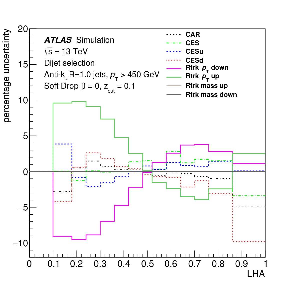 Figure 1
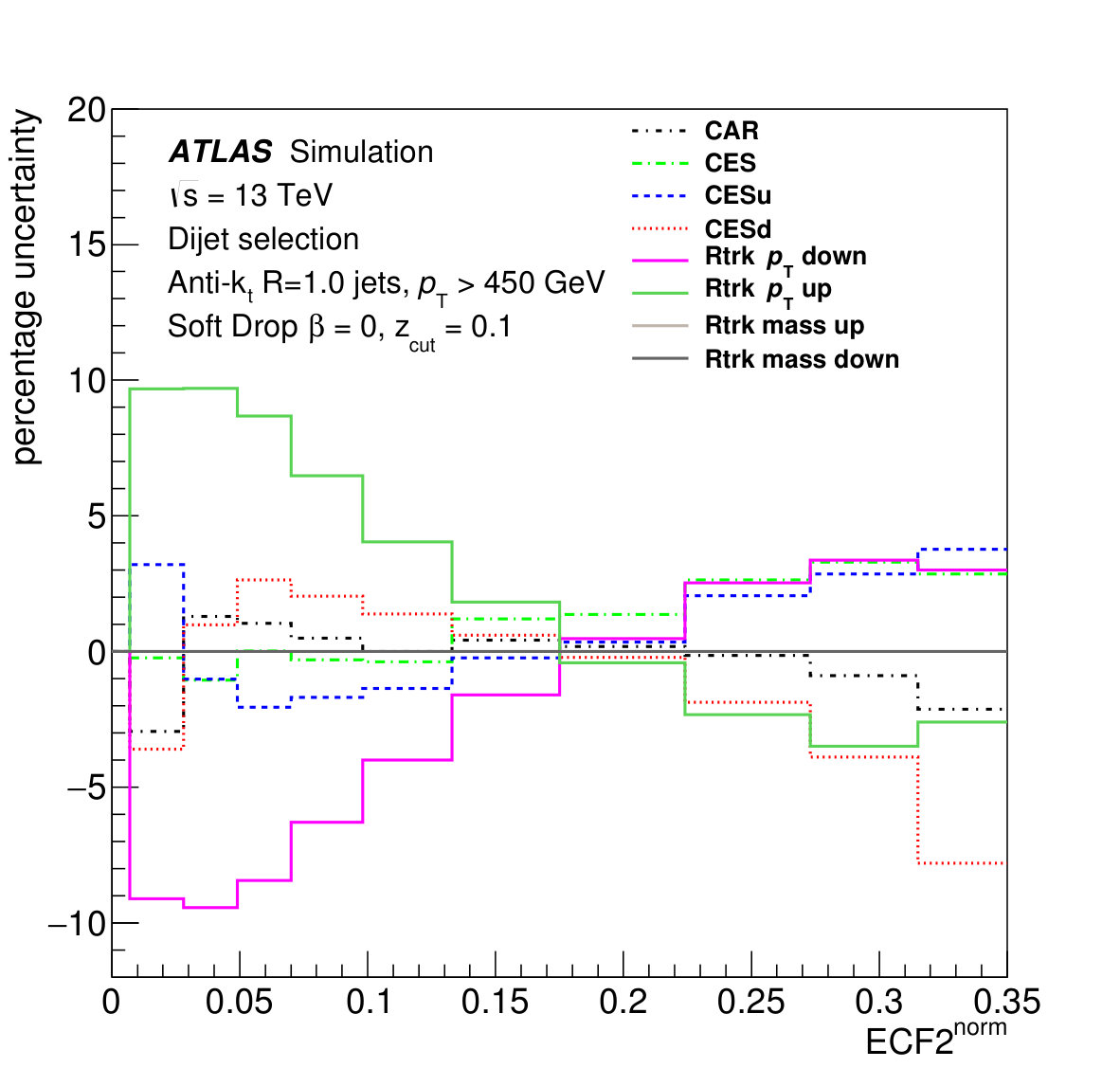 Figure 1
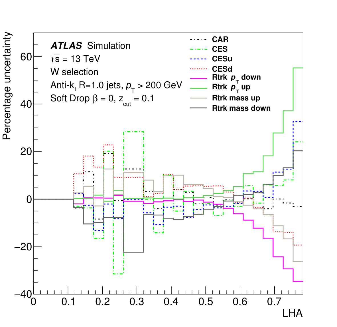 Figure 1
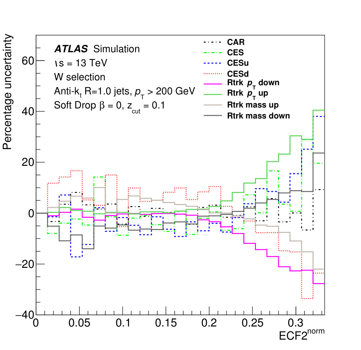 Figure 1
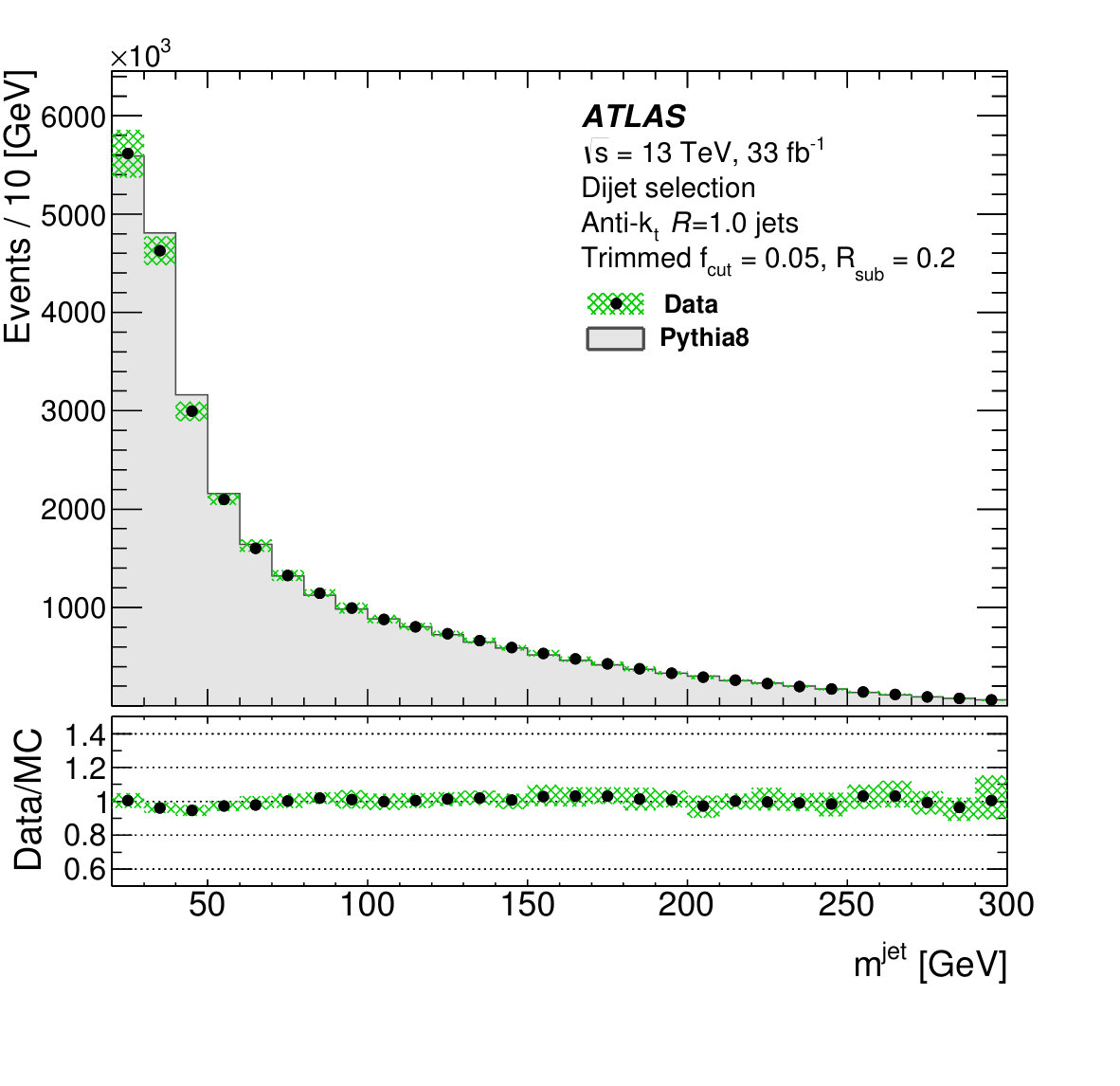 Figure 2
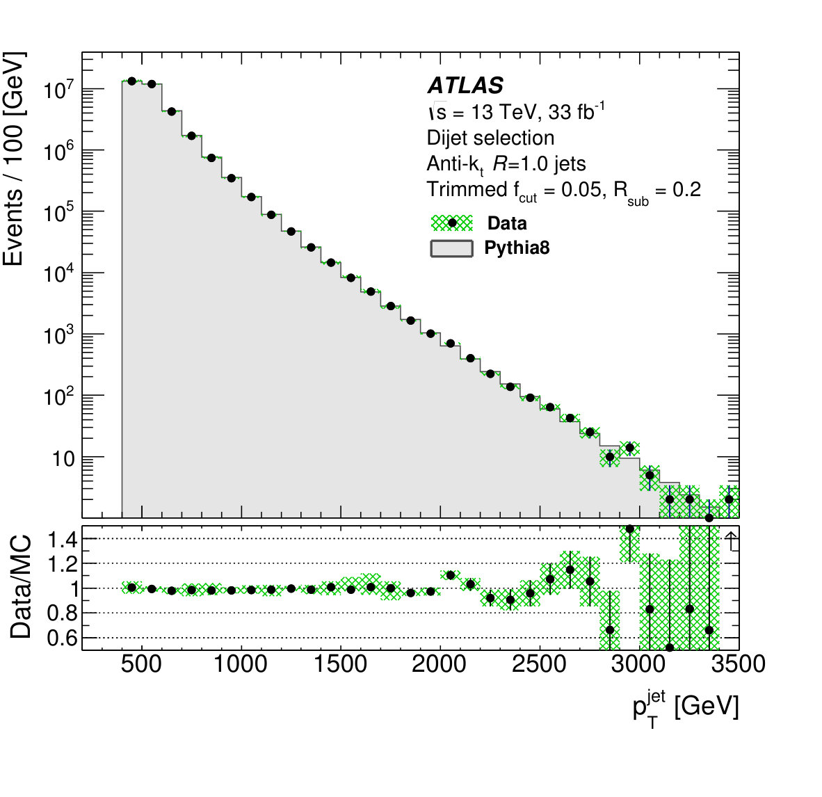 Figure 2
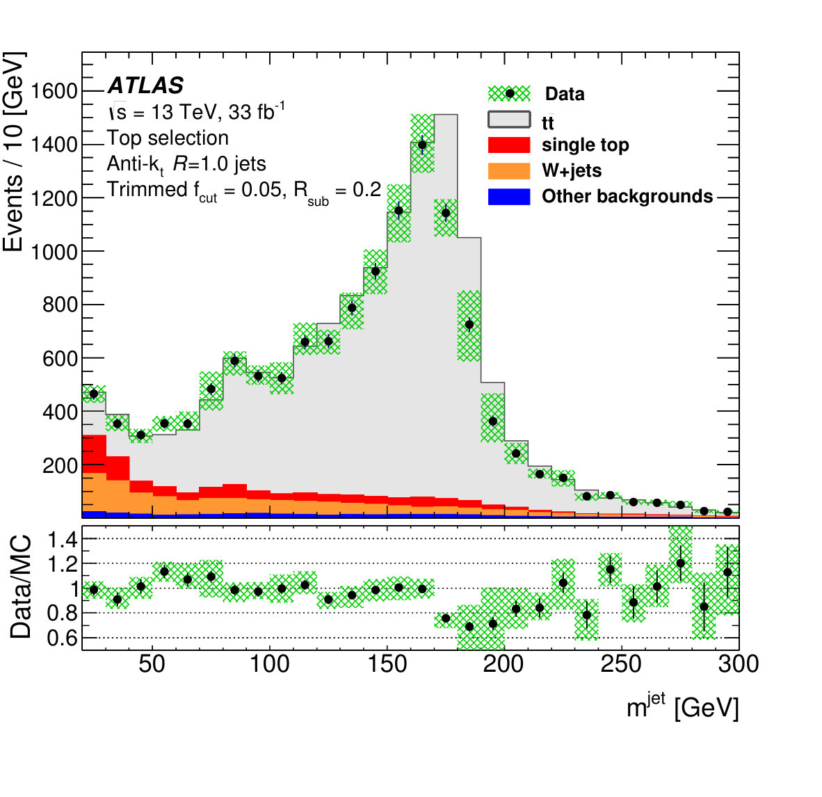 Figure 2
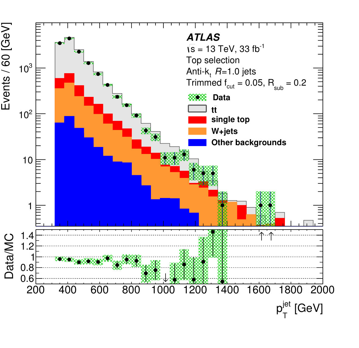 Figure 2
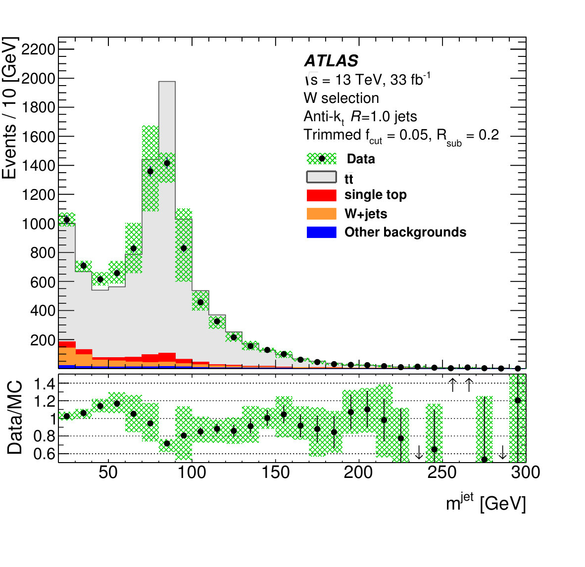 Figure 2
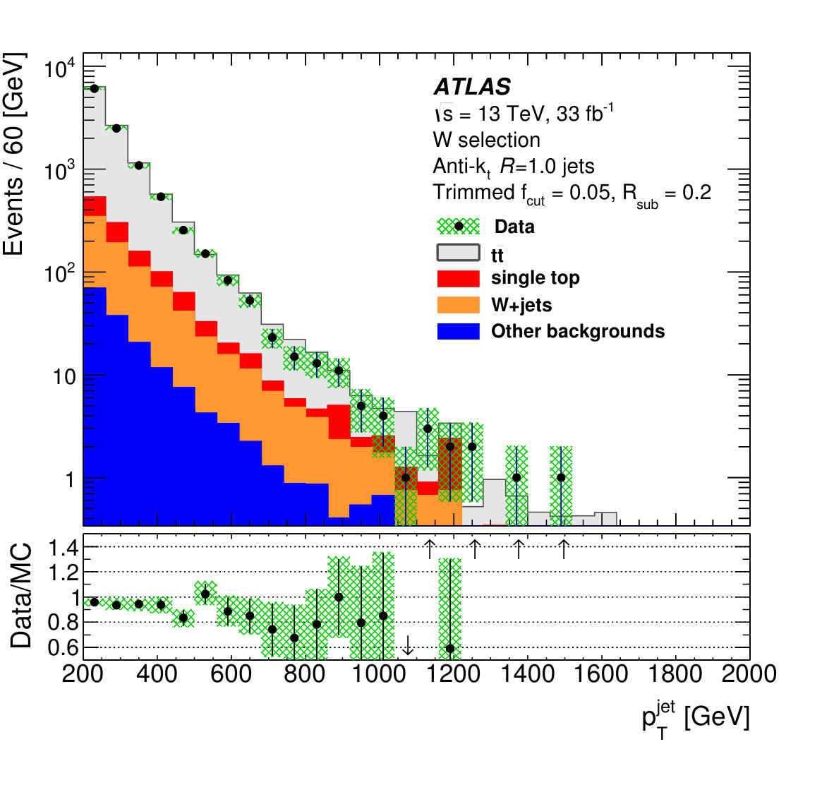 Figure 2
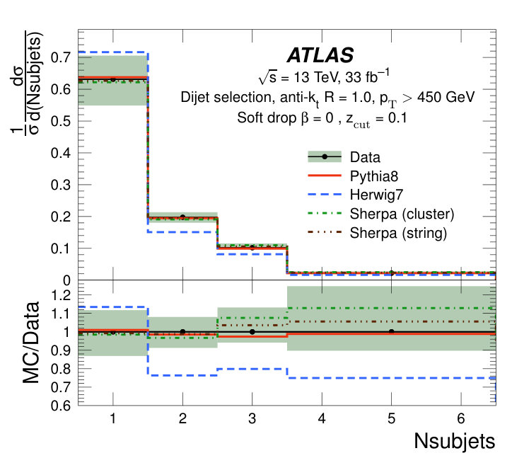 Figure 3
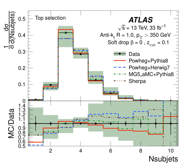 Figure 3
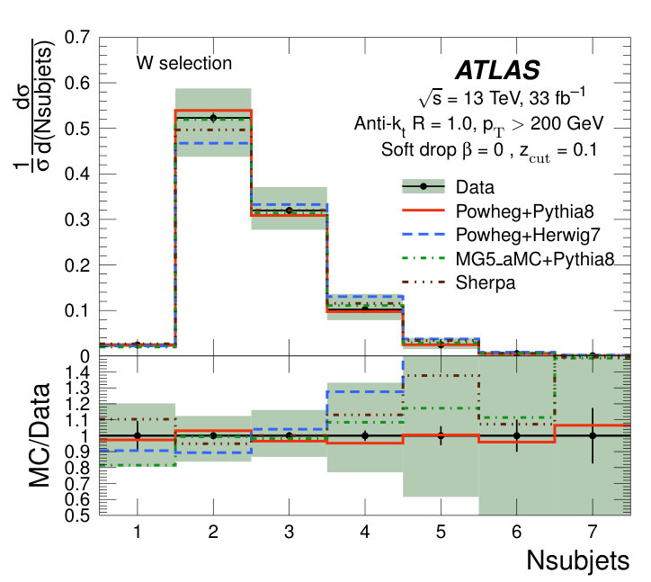 Figure 3
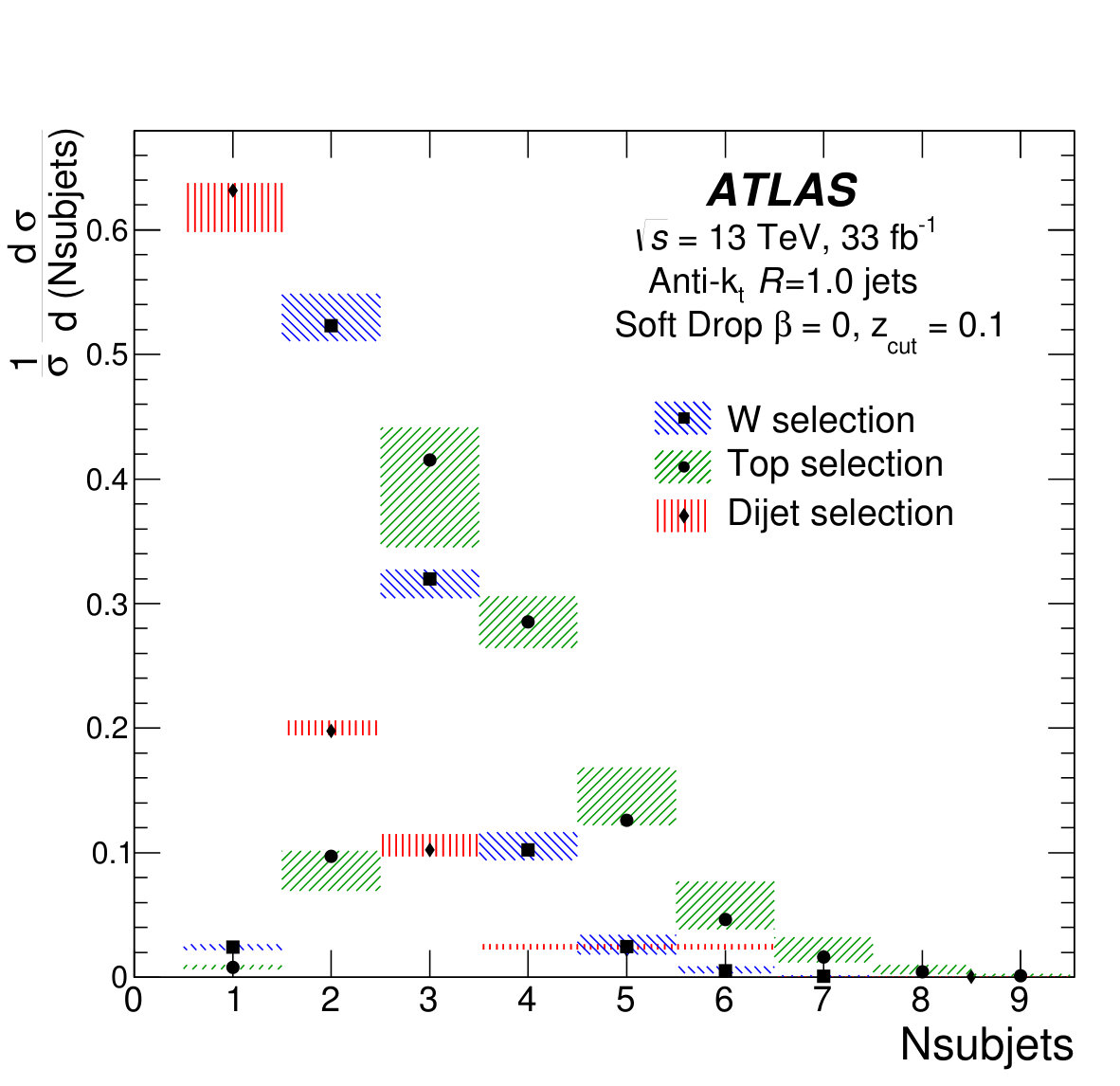 Figure 3
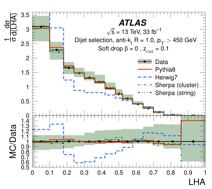 Figure 4
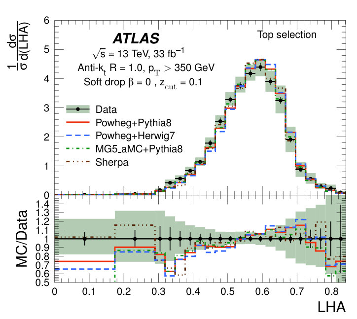 Figure 4
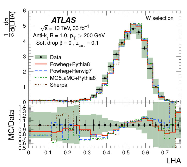 Figure 4
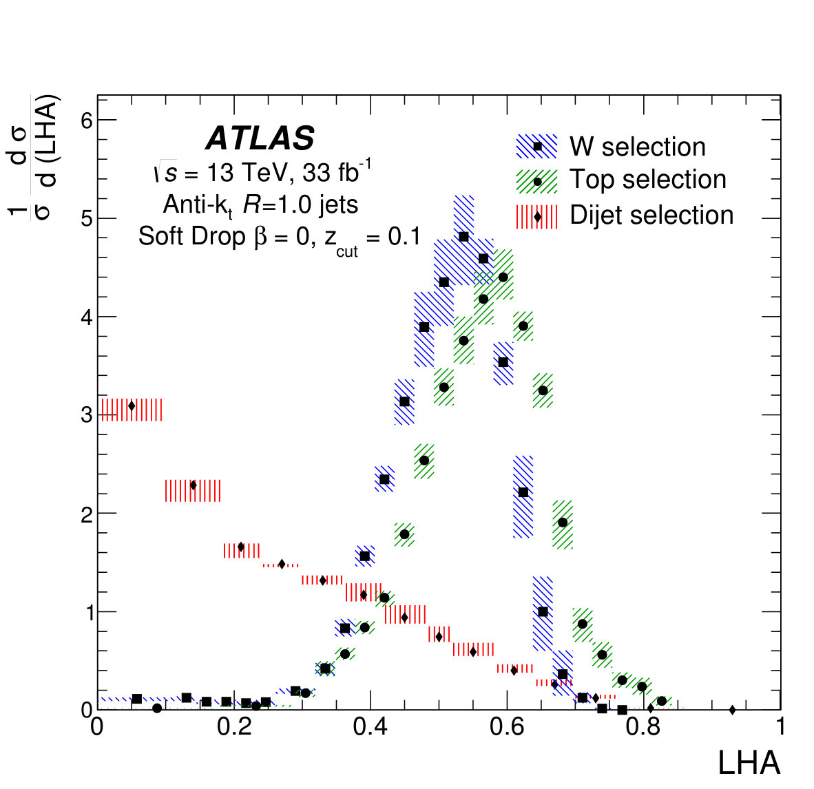 Figure 4
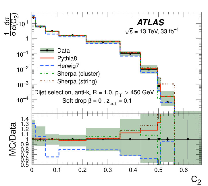 Figure 5
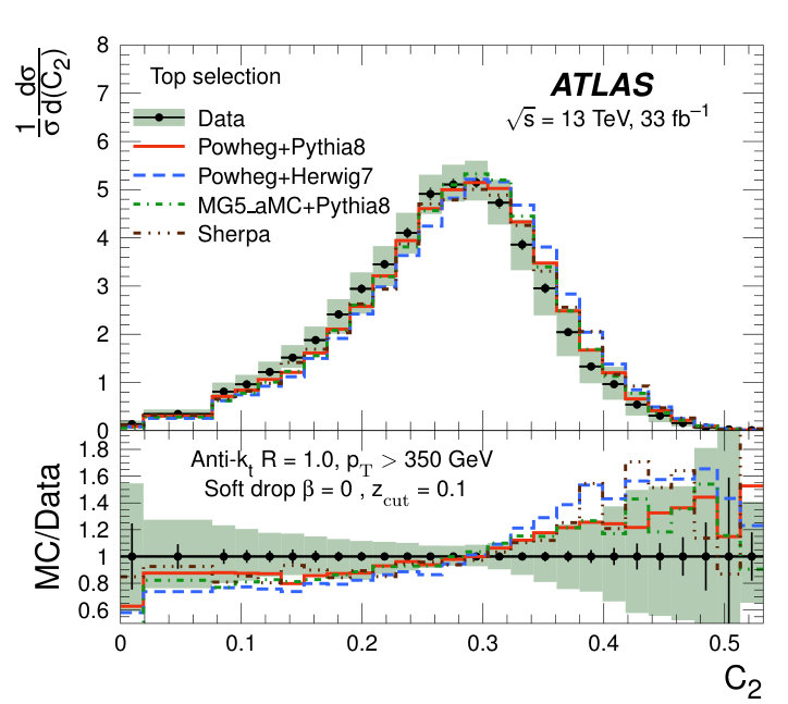 Figure 5
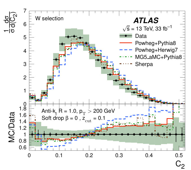 Figure 5
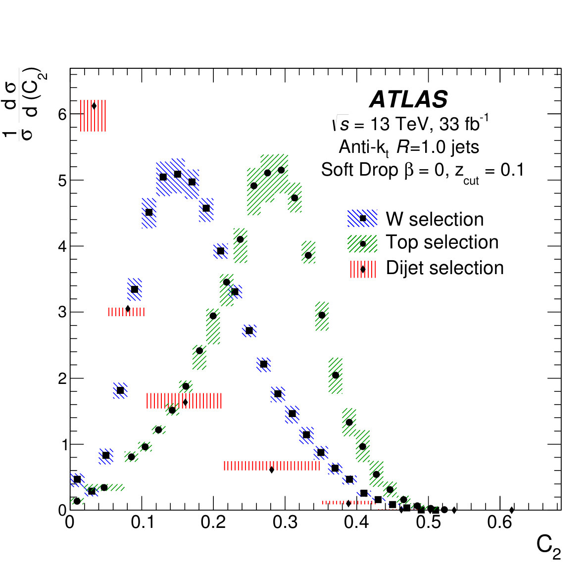 Figure 5
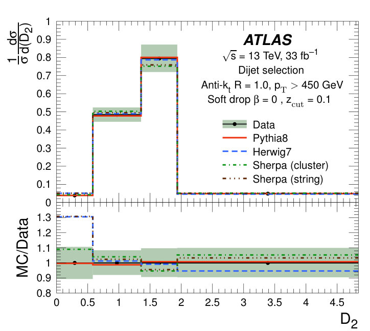 Figure 6
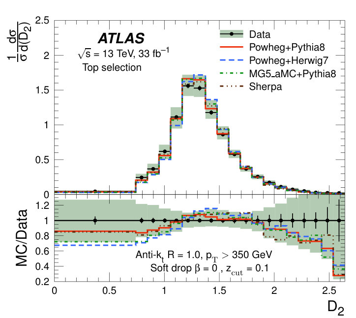 Figure 6
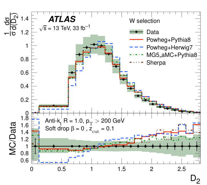 Figure 6
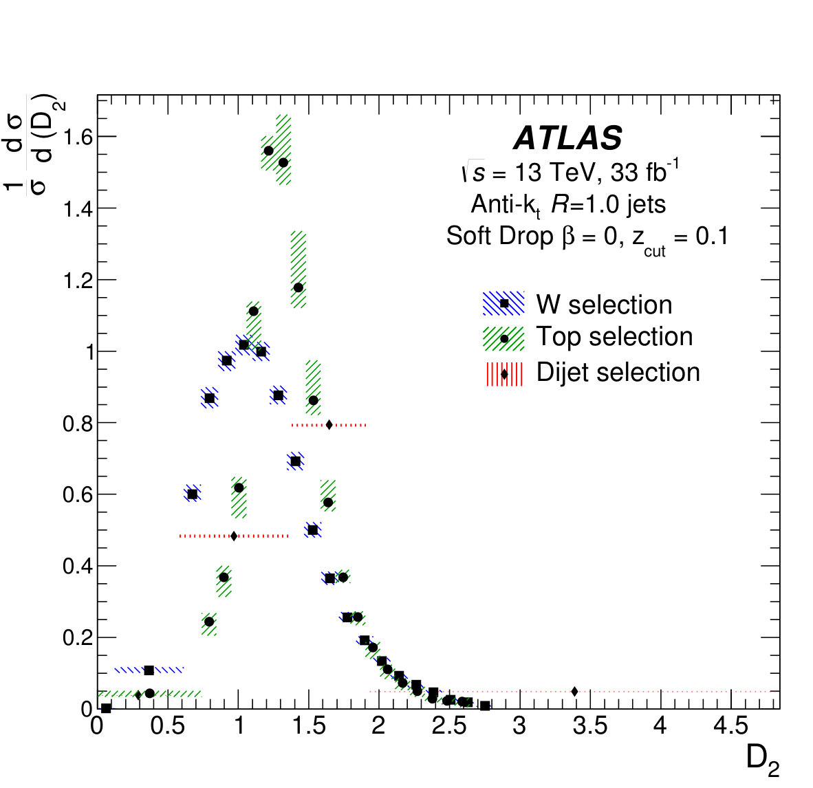 Figure 6
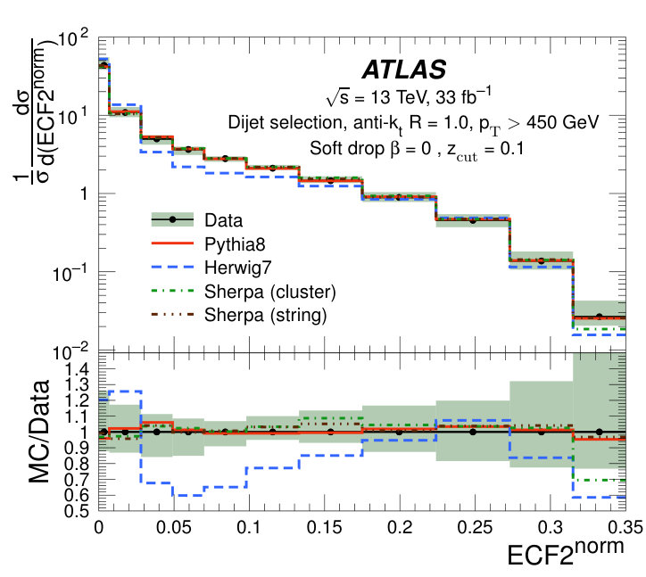 Figure 7
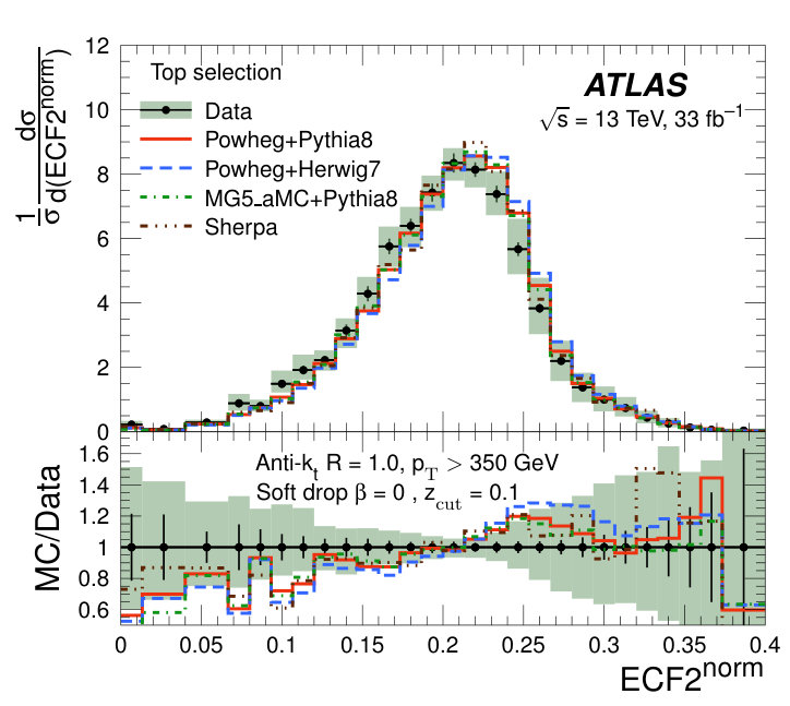 Figure 7
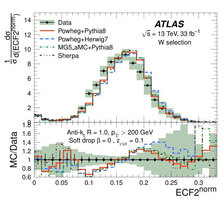 Figure 7
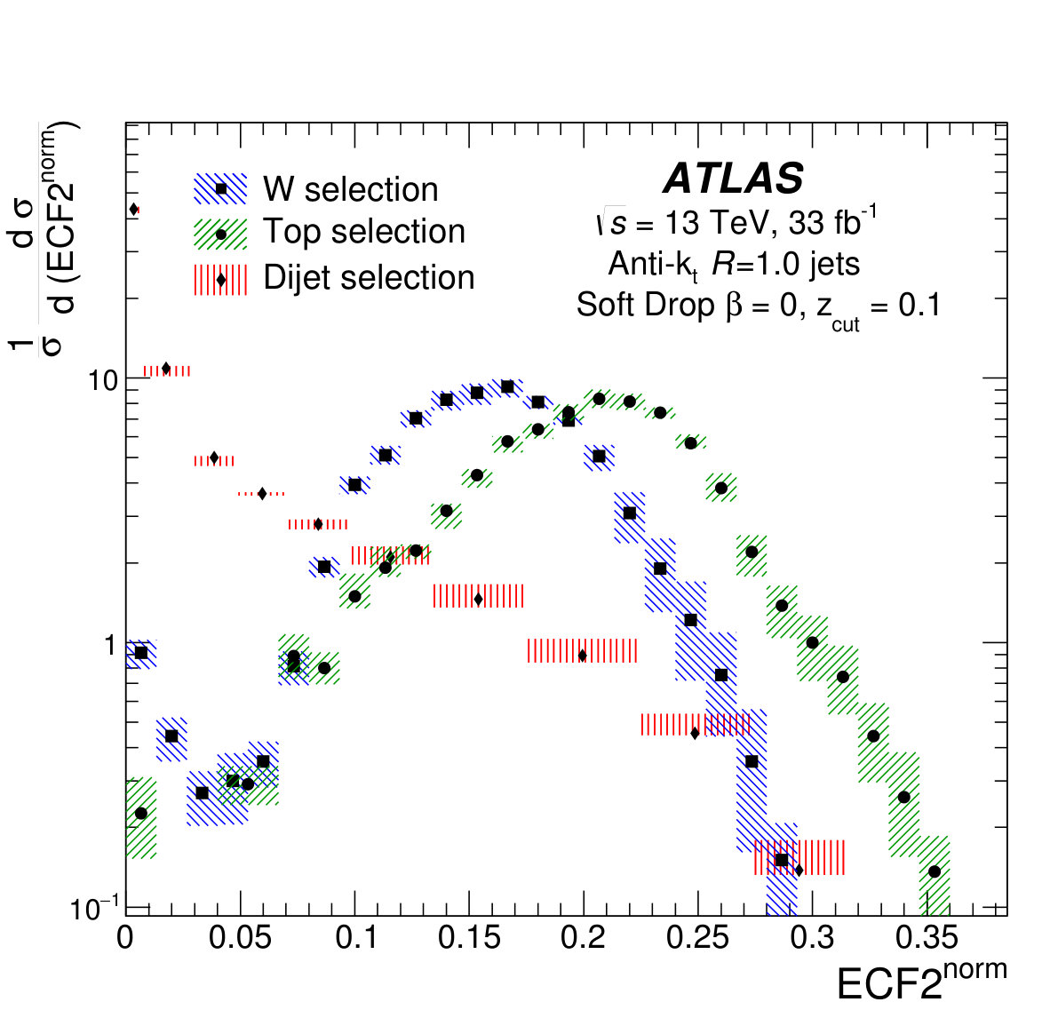 Figure 7
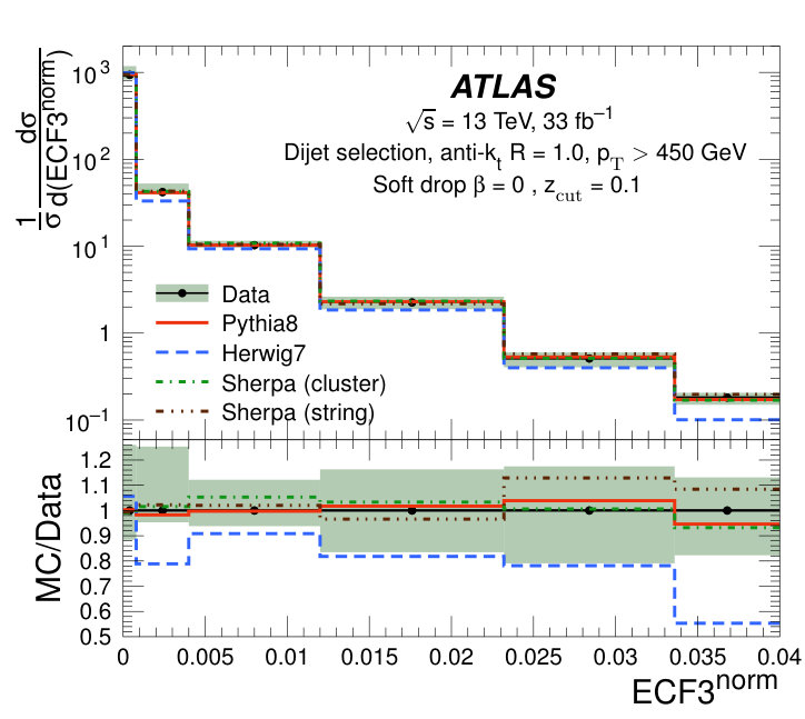 Figure 8
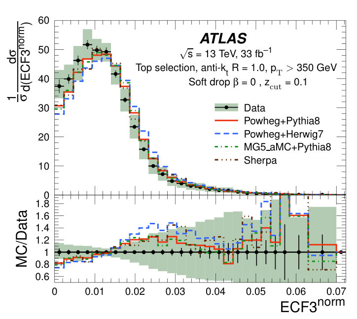 Figure 8
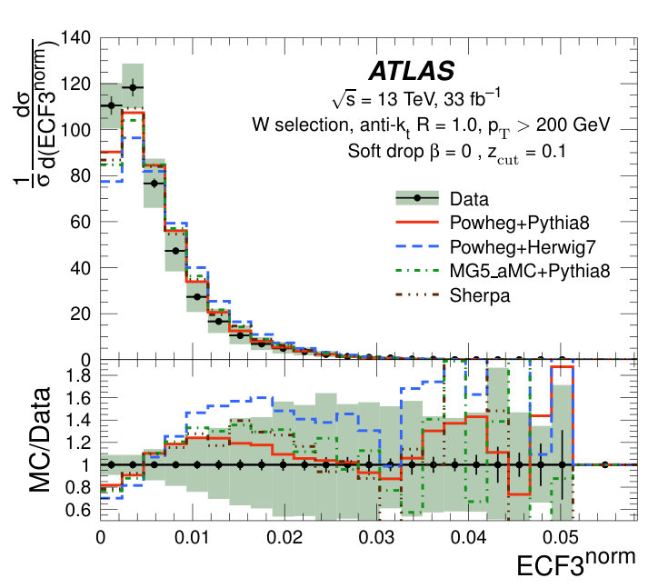 Figure 8
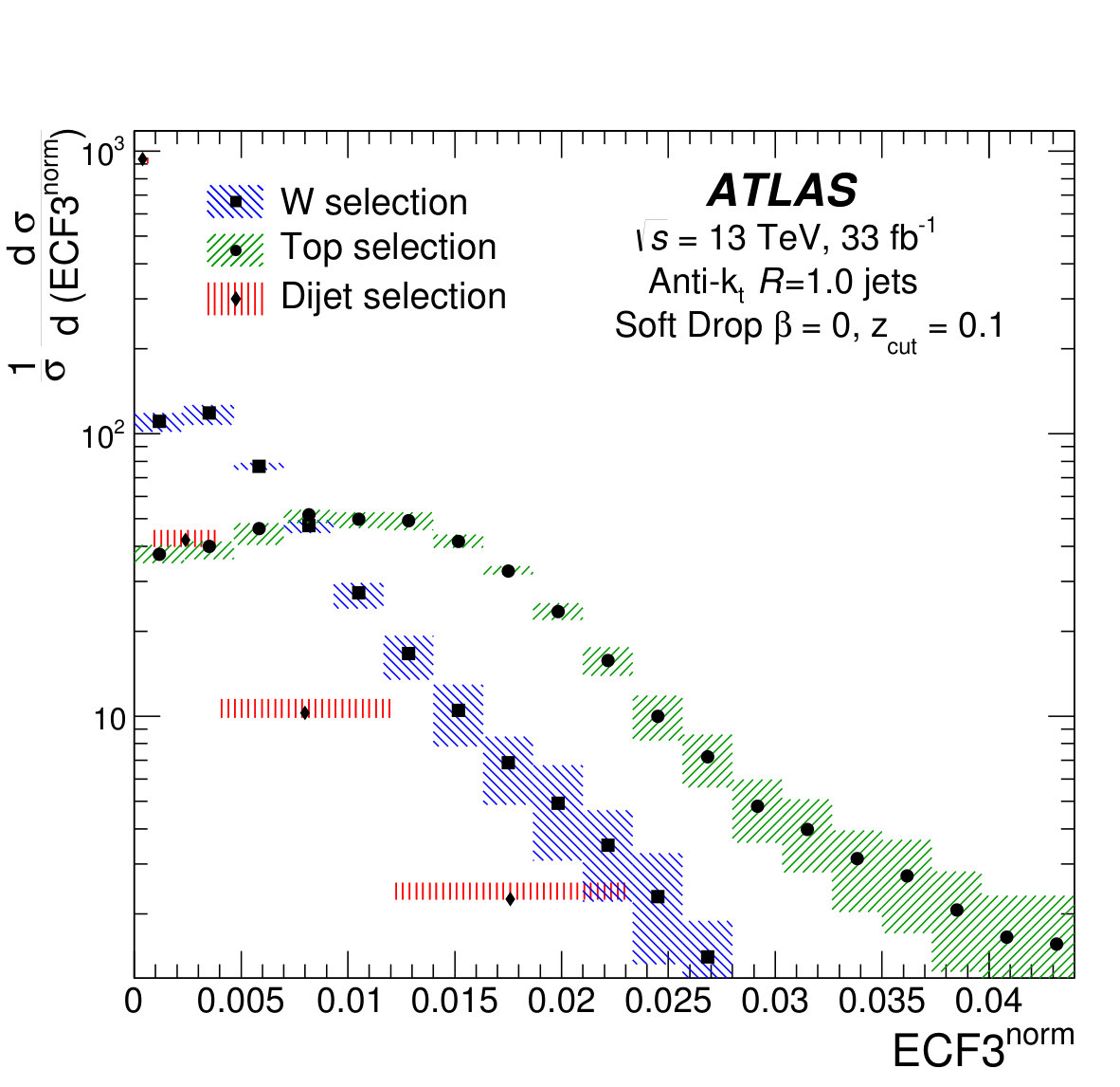 Figure 8
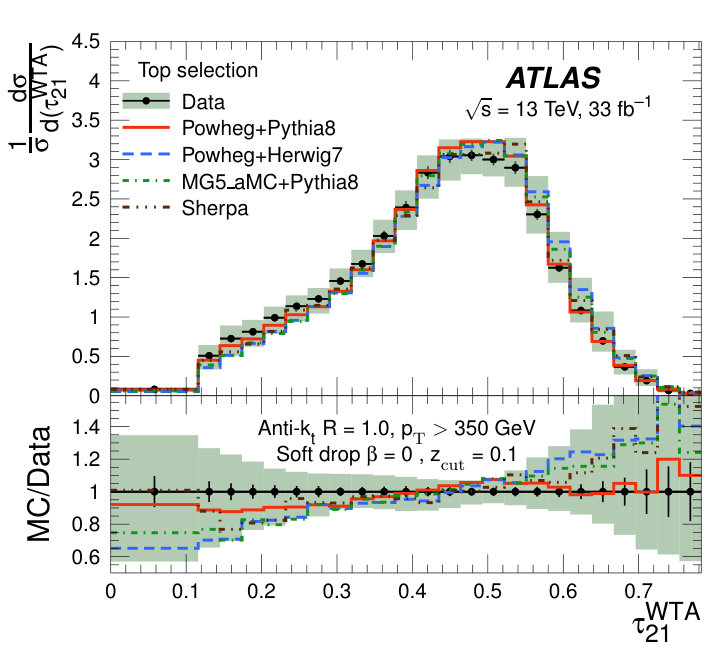 Figure 9
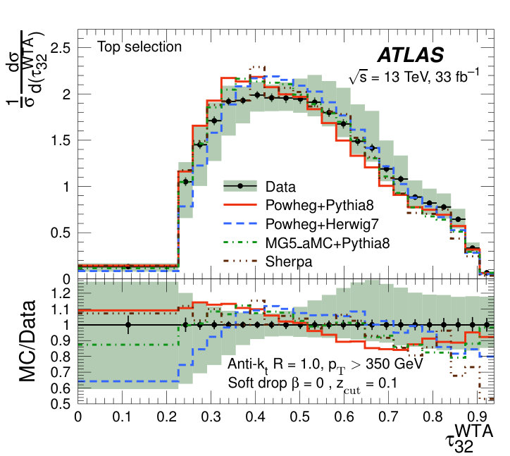 Figure 9
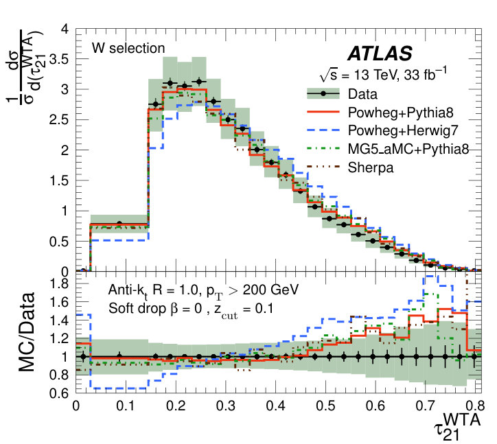 Figure 9
| Process | Generator | Version | Tune | Use | |
| Dijet | Pythia8 [40, 41] | 8.186 | NNPDF23LO [42] | A14 [43] | Nominal for unfolding |
| Sherpa [44] | 2.2.1 | CT10 [45] | Default | Validation of unfolding | |
| (with two different hadronisation models) | |||||
| Herwig7 [46] | 7.0.4 | MMHT2014 | H7UE [46] | Comparison | |
| Powheg [47] | v2 | NNPDF30NLO | Nominal for unfolding | ||
| + Pythia8 | 8.186 | NNPDF23LO | A14 | ||
| Powheg | v2 | CT10 | Validation of unfolding | ||
| +Herwig [48] | 2.7 | CTEQ6L1 | UE-EE-5 tune [49] | ||
| Powheg | v2 | CT10 | Comparison | ||
| +Herwig7 | 7.0.4 | MMHT2014 | H7UE | ||
| MG5_aMC@NLO [50] | 2.6.0 | NNPDF30NLO | Comparison | ||
| + Pythia8 | 8.186 | NNPDF23LO | A14 | ||
| Sherpa | 2.2.1 | CT10 | Default | Comparison | |
| Single top | Powheg | v1 | CT10 | Nominal for unfolding | |
| + Pythia6 [51, 52] | 6.428 | CTEQ6L1 [45] | Perugia2012 [53] | ||
| +jets | Sherpa | 2.2.1 | CT10 | Default | Background estimation |
| +jets | Sherpa | 2.2.1 | CT10 | Default | Background estimation (nominal) |
| +jets | MG5_aMC@NLO | 2.2.5 | CT10 | Background estimation (cross-check) | |
| + Pythia8 | 8.186 | NNPDF23LO | A14 | ||
| Diboson | Sherpa | 2.2.1 | CT10 | Default | Background estimation |
| Detector level | Particle level | |
| Dijet selection: | ||
| Two trimmed anti- jets | GeV | GeV |
| Leading- trimmed anti- jet | GeV | |
| Top and selections: | ||
| Exactly one muon | GeV | GeV |
| mm and | ||
| Anti- jets | GeV | GeV |
| (if GeV) | ||
| Muon isolation criteria | If : | None |
| muon is removed, so the event is discarded | ||
| , | 20 GeV, + 60 GeV | |
| Leptonic top | At least one small-radius jet with | |
| Top selection: | ||
| Leading- trimmed anti- jet | , GeV, GeV | |
| selection: | ||
| Leading- trimmed anti- jet | , GeV, GeV and GeV | |
| Background | Top selection | selection |
|---|---|---|
| (Percent contributions) | ||
| +jets | 4.0 0.1 | 2.6 0.1 |
| Misreconstructed and non-prompt muons | 6.6 0.1 | 5.5 0.1 |
Peer Reviews
No public reviews on file for this paper yet. If you reviewed it on a platform where reviews are public (OpenReview, ICLR, NeurIPS, ICML), you can paste yours below so the community can read it here.
Videos
No videos yet. Explain this paper in a talk, walkthrough, or lecture? Add one.
\AtlasTitle
Measurement of jet-substructure observables in top quark, boson and light jet production in proton-proton collisions at TeV with the ATLAS detector
\PreprintIdNumberCERN-EP-2019-011 \AtlasRefCodeSTDM-2017-34 \AtlasJournalRefJHEP 08 (2019) 033 \AtlasDOI10.1007/JHEP08(2019)033 \AtlasAbstract A measurement of jet substructure observables is presented using data collected in 2016 by the ATLAS experiment at the LHC with proton-proton collisions at TeV. Large-radius jets groomed with the trimming and soft-drop algorithms are studied. Dedicated event selections are used to study jets produced by light quarks or gluons, and hadronically decaying top quarks and bosons. The observables measured are sensitive to substructure, and therefore are typically used for tagging large-radius jets from boosted massive particles. These include the energy correlation functions and the -subjettiness variables. The number of subjets and the Les Houches angularity are also considered. The distributions of the substructure variables, corrected for detector effects, are compared to the predictions of various Monte Carlo event generators. They are also compared between the large-radius jets originating from light quarks or gluons, and hadronically decaying top quarks and bosons.
1 Introduction
Increasing the centre-of-mass energy of proton–proton () collisions from 7 and 8 TeV in Run 1 to 13 TeVi̇n Run 2 of the Large Hadron Collider (LHC) leads to a larger fraction of heavy particles such as top quarks, vector bosons and Higgs bosons being produced with large transverse momenta. This large transverse momentum leads to collimated decay products. They are usually reconstructed in a large-radius jet, whose internal (sub)structure shows interesting features that can be used to identify the particle that initiated the jet formation [1, 2].
This is relevant for a host of measurements and searches, which involve identifying the large-radius jets coming from top quarks [3, 4, 5, 6, 7]. or Higgs bosons [8, 9, 10, 11], for example in Run 2 in ATLAS. Usually a two step procedure is employed. In the first step, termed grooming, the effect of soft, uncorrelated radiation contained in the large-radius jet in reduced. Then jet substructure observables, which describe the spatial energy distribution inside the jets, are used to classify the jets originating from different particles. This process is called jet tagging and the algorithms are referred to as taggers.
Most of the grooming algorithms and jet substructure observables were developed on the basis of theoretical calculations or Monte Carlo (MC) simulation programs and then t hey are applied to data. Given that often large differences have been seen between predictions from MC and data, large correction factors need to be applied to simulation results. Additionally, taggers suffer from large systematic uncertainties as the modelling of the substructure observables is not well constrained [12, 2]. Most of these variables have never been measured in data, and performing a proper unfolded measurement is a common request from the theory community. Measuring these observables will help in optimising and developing current and future substructure taggers, as well as tuning hadronization models in the important but still relatively unexplored regime of jet substructure. The choice of variables measured in this paper prioritized jet shapes commonly used in jet tagging, as well as those most useful for model tuning.
The ATLAS Collaboration has performed measurements of jet mass and substructure variables at the centre-of-mass energies of , and TeV [13, 14, 15, 16, 17, 18, 19] in inclusive jet events, and the CMS Collaboration has performed measurements of jet mass and substructure in dijet, / boson, and events [20, 21, 22, 23, 24] at , and TeV. This paper presents measurements of substructure variables in large-radius jets produced in inclusive multijet events and in events at TeV using fb*-1* of data collected in 2016 by the ATLAS experiment. In this analysis, the lepton+jets decay mode of events is selected, where one boson decays into a muon and a neutrino, and the other boson decays into a pair of quarks. Then the large-radius jets are separated into those that contain all the decay products of a hadronically top quark and those containing only hadronic boson decay products.
The contents of this paper are organised as follows. First, a description of the ATLAS detector is presented in Section 2 and then the MC samples used in the analysis are discussed in Section 3. In Section 4, event and object selections are summarised. The measured jet substructure observables are defined in Section 5. The background estimation is described in Section 6 and the systematic uncertainties are assessed in Section 7. In Section 8, detector-level mass and distributions corresponding to selected large-radii jets are shown, and the unfolding is described in Section 9. Finally, the unfolded results are presented in Section 10, and the conclusions in Section 11.
2 ATLAS detector
The ATLAS experiment uses a multipurpose particle detector [25, 26] with a forward–backward symmetric cylindrical geometry and a near coverage in solid angle.111 ATLAS uses a right-handed coordinate system with its origin at the nominal interaction point (IP) in the centre of the detector and the -axis along the beam pipe. The -axis points from the IP to the centre of the LHC ring, and the -axis points upwards. Cylindrical coordinates are used in the transverse plane, being the azimuthal angle around the -axis. The pseudorapidity is defined in terms of the polar angle as . An angular separation between two objects is defined as , where and are the separations in and . Momentum in the transverse plane is denoted by . It consists of an inner tracking detector (ID) surrounded by a thin superconducting solenoid providing a T axial magnetic field, electromagnetic (EM) and hadron calorimeters, and a muon spectrometer. The ID consists of silicon pixel, silicon microstrip, and straw-tube transition-radiation tracking detectors, covering the pseudorapidity range . The calorimeter system covers the pseudorapidity range . Electromagnetic calorimetry is performed with barrel and endcap high-granularity lead/liquid-argon (LAr) sampling calorimeters, within the region . There is an additional thin LAr presampler covering , to correct for energy loss in material upstream of the calorimeters. For , the LAr calorimeters are divided into three layers in depth. Hadronic calorimetry is performed with a steel/scintillator-tile calorimeter, segmented into three barrel structures within , and two copper/LAr hadronic endcap calorimeters, which cover the region . The forward solid angle up to is covered by copper/LAr and tungsten/LAr calorimeter modules, which are optimised for energy measurements of electrons/photons and hadrons, respectively. The muon spectrometer consists of separate trigger and high-precision tracking chambers that measure the deflection of muons in a magnetic field generated by superconducting air-core toroids.
The ATLAS detector selects events using a tiered trigger system [27]. The first level is implemented in custom electronics. The second level is implemented in software running on a general-purpose processor farm which processes the events and reduces the rate of recorded events to 1 kHz.
3 Monte Carlo samples
Simulated events are used to optimise the event selection, correct the data for detector effects and estimate systematic uncertainties. The predictions of different phenomenological models implemented in the Monte Carlo (MC) generators are compared with the data corrected to the particle level (i.e. observables constructed from final-state particles within the detector acceptance).
The generators used to produce the samples are listed in Table 1. The dijet (to obtain multijet events), and single-top-quark samples are considered to be signal processes in this analysis, corresponding to the dedicated selections. The background is estimated using +jets and diboson samples. The samples are scaled to next-to-next-to-leading order (NNLO) in perturbative QCD, including soft-gluon resummation to next-to-next-to-leading-log order (NNLL) [28] in cross-section, assuming a top quark mass GeV. The Powheg model [29] resummation damping parameter, , which controls the matching of matrix elements to parton showers and regulates the high- radiation, was set to [30]. The single-top-quark [31, 32, 33, 34, 35, 36] and samples [37] are scaled to the NNLO theoretical cross-sections.
The predicted shape of jet substructure distributions depends on the modelling of final-state radiation (FSR), and fragmentation and hadronisation, as well as on the merging/matching between matrix element (ME) and parton shower (PS) generators. The Pythia8 and the Sherpa generators use a dipole shower ordered in transverse momentum, with the Lund string [38] and cluster hadronisation model [39] respectively. The Herwig7 generator uses an angle-ordered shower, with the cluster hadronisation model. For comparison purposes in dijet events, a sample was generated with Sherpa using the string hadronisation model.
The MC samples were processed through the full ATLAS detector simulation [54] based on Geant4 [55], and then reconstructed and analysed using the same procedure and software that are used for the data. Additional collisions generated by Pythia8, with parameter values set to the A2 tune [56] and using the MSTW2008 [57] PDF set, were overlaid to simulate the effects of additional collisions from the same and nearby bunch crossings (pile-up), with a distribution of the number of extra collisions matching that of data.
4 Object and event selection
This analysis uses collision data at TeV collected by the ATLAS detector in 2016, that satisfy a number of criteria to ensure that the ATLAS detector was in good operating condition. All selected events must have at least one vertex with at least two associated tracks with MeV. The vertex with the highest , where is the transverse momentum of a track associated with the vertex, is chosen as the primary vertex.
Jets are reconstructed from the EM-scale or locally-calibrated topological energy clusters [58] in both the EM and hadronic calorimeters using the anti- algorithm [59] with a radius parameter of or , referred to as small-radius and large-radius jets respectively. These clusters are assumed to be massless when computing the jet four-vectors and substructure variables. A trimming algorithm [60] is employed for the large-radius jets to mitigate the impact of initial-state radiation, underlying-event activity, and pile-up. Trimming removes subjets of radius with , where is the transverse momentum of the subjet, is the transverse momentum of the jet under consideration, and . All large-radius jets used in this paper are trimmed before applying the selection criteria. The energies of jets are calibrated by applying - and rapidity-dependent corrections derived from Monte Carlo simulation with additional correction factors for residual non-closure in data determined from data [58, 61].
In order to reduce the contamination by small-radius jets originating from pile-up, a requirement is imposed on the output of the Jet Vertex Tagger (JVT) [62]. The JVT algorithm is a multivariate algorithm that uses tracking information to reject jets which do not originate from the primary vertex, and is applied to jets with GeV and . Small-radius jets containing -hadrons are tagged using a neural-network-based algorithm [63, 64, 65] that combines information from the track impact parameters, secondary vertex location, and decay topology inside the jets. The operating point corresponds to an overall efficiency in simulated events, and to a probability of mis-tagging light-flavour jets of approximately .
Muons are reconstructed from high-quality muon spectrometer track segments matched to ID tracks. Muons with a transverse momentum greater than 30 GeV and within are selected if the associated track has a longitudinal impact parameter mm and a transverse impact parameter significance . The impact parameter is measured relative to the beam line. The muon candidates are also required to be isolated from nearby hadronic activity [66]. The muon isolation criteria remove muons that lie a distance from a small-radius jet axis, where is the of the muon. Since muons deposit energy in the calorimeters, an overlap removal procedure is applied in order to avoid double counting of leptons and small-radius jets.
Electrons are reconstructed from energy deposits measured in the EM calorimeter which are matched to ID tracks. They are required to be isolated from nearby hadronic activity by using a set of - and -dependent criteria based on calorimeter and track information as described in Ref. [67]. Their selection also requires GeV and , excluding the region which corresponds to the transition region between the barrel and end-cap calorimeters. Photon candidates are reconstructed from clusters of energy deposited in the EM calorimeter, and must have GeV and . Photon identification is based primarily on shower shapes in the calorimeter [68].
The missing transverse momentum, with magnitude , is calculated as the negative vectorial sum of the transverse momenta of calibrated photons, electrons, muons and jets associated with the primary vertex [69]. The transverse mass of the leptonically decaying boson, , is defined using the absolute value of as m_{\mathrm{T}}^{\mathrm{W}}=\sqrt{2p_{\mathrm{T},\mu}E_{\text{T}}^{\text{miss}}\big{(}1-\cos\Delta\phi(\mu,E_{\text{T}}^{\text{miss}})\big{)}}.
In order to examine large-radius jets originating from light quarks and gluons, from top quarks and from bosons, three event selections are defined. These are referred to as dijet, top and * selections*, and are indicative of the origin of the large-radius jet.
In the dijet selection, the events are accepted by a single-large-radius-jet trigger that becomes fully efficient for jets with GeV. The offline dijet selection requires a leading trimmed large-radius jet with GeV and , and at least one other trimmed large-radius jet with GeV and , and rejects the event if an electron or muon is present.
For both the top and selections, events are collected with a set of single-muon triggers that become fully efficient for muon GeV. The top quarks and the bosons are identified from their decay products. A geometrical separation between the decay products of the two top quark candidates is required. Additional requirements are applied to separate large-radius jets containing all decay products of the top quark from those where the large-radius jet only contains the hadronic boson decays, with the small-radius jet reconstructed independently. These form the top selection and the selection respectively. The selections are described in Table 2. After these requirements the data sample contains about events in the dijet selection, and roughly 6800 and 4500 events in the top and selection respectively.
Particle-level observables in Monte Carlo simulation are constructed from stable particles, defined as those with proper lifetimes mm. Muons at particle level are dressed by including contributions from photons with an angular distance from the muon. Particle-level jets do not include muons or neutrinos. Particle-level -tagging is performed by requiring a prompt -hadron to be ghost-associated [70] with the jet.
5 Definition of the jet observables
All large-radius jets are trimmed before being used in the selections, and subsequently only the leading trimmed large-radius is considered in the analysis. Then the large-radius jet constructed from the original constituents of the selected jet before the trimming step is groomed using the soft-drop algorithm, and the jet substructure observables studies are constructed from that soft-dropped large-radius jet.
Soft-drop [71, 72] is an extension of the original split-filtering technique [73] and relies on reclustering the jet constituents using the angle-ordered Cambridge–Aachen jet algorithm and then sequentially considering each splitting in order to remove soft and wide-angle radiation. At each step the jet is split into two proto-jets. The removal of proto-jets in a splitting is controlled by two parameters: a measure of the energy balance of the pair, , and the significance of the angular separation of the proto-jets, . These are used to define the soft-drop condition:
[TABLE]
where is the angular distance between the two proto-jets and is the radius of the large jet. In this analysis, values of and are used, based on previous ATLAS studies [18], which is equivalent to modified mass drop tagger [74]. An important feature of soft-drop is that groomed observables are analytically calculable to high-order resummation accuracy [75, 76, 77].
The following substructure variables are measured in this analysis:
- •
Number of subjets with GeV, reconstructed from the selected large-radius jet constituents using the algorithm [78] with .
- •
Generalised angularities defined as:
[TABLE]
where is the transverse momentum of jet constituent as a fraction of the scalar sum of the of all constituents and is the angle of the constituent relative to the jet axis, normalised by the jet radius. The exponents and probe different aspects of the jet fragmentation. The variant is termed the Les Houches angularity (LHA) [79] and used in this analysis. It is an infrared-safe version of the jet-shape angularity, and provides a measure of the broadness of a jet.
- •
Energy correlation functions ECF2 and ECF3 [80], and related ratios , [81]. The 1-point, 2-point and 3-point energy correlation functions for a jet are given by:
[TABLE]
where the parameter weights the angular separation of the jet constituents. In the above functions, the sum is over the constituents in the jet , such that the 1-point correlation function ECF1 is approximately the jet . Likewise, if one takes , the 2-point correlation functions scale as the mass of a particle undergoing a two-body decay in collider coordinates. In this analysis, is used, and for brevity, is not explicitly mentioned hereafter.
The ratios of some of these quantities (written in an abbreviated form) are defined as :
[TABLE]
The observables and are measured, and are later referred to as and . These ratios are then used to generate the variable [80], and its modified version [79, 81], which have been shown to be particularly useful in identifying two-body structures within jets [82]. The and variables as defined below are measured in this analysis:
[TABLE]
- •
Ratios of -subjettiness [83], and . The -subjettiness describes to what degree the substructure of a given jet is compatible with being composed of or fewer subjets.
In order to calculate , first subjet axes are defined within the jet by using the exclusive algorithm, where the jet reconstruction continues until a desired number of jets are found. The 0-, 1-, 2-,and 3-subjettiness are defined as:
[TABLE]
where is the angular distance between constituent and the jet axis, , and is the angular distance between constituent and the axis of the subjet. The term in equation 1a is the radius parameter of the jet. The parameter gives a weight to the angular separation of the jet constituents. In the studies presented here, the value of is used. In the above functions, the sum is performed over the constituents in the jet , and a normalisation factor (Eq. (1a)) is used. The ratios of the -subjettiness functions, and have been shown to be particularly useful in identifying two-body and three-body structures within jets.
Studies presented in Ref. [84] have shown that an alternative axis definition can increase the discrimination power of these variables. The winner-takes-all (WTA) axis uses the direction of the hardest constituent in the subjet obtained from the exclusive algorithm instead of the subjet axis, such that the distance measure changes in the calculation. In this analysis, the same observables calculated with the WTA axis definition, and , are used.
6 Data-driven background estimation
The largest non- contributions to the and top selections come from the +jets and single-top processes. Additionally non-prompt and mis-reconstructed muons are a separate source of background for the top and selections. Contributions from other processes were considered and found to be negligible. A data-driven method, following Ref. [85], is used to estimate the contribution from the +jets process while the single-top process is considered part of the signal.
At the LHC the production rate of +jets events is larger than that of +jets due to the higher density of -quarks than -quarks in the proton. This results in more events with positively charged leptons. Other processes do not contribute significantly to this charge asymmetry. The data are used to derive scale factors that correct the normalisation and flavour fraction given by the MC simulation [86].
Normalisation scale factors are determined by comparing the charge asymmetry in data with the asymmetry estimated by simulation. Contributions to the asymmetry from other processes are estimated by simulation and subtracted. A selection that contains the full top and selection criteria without any -tagging requirements is initially used. The total number of +jets events in data, , is given by
[TABLE]
where is the ratio of the number of events with positive muons to the number of events with negative muons obtained from the MC simulation while and are the number of events with positive and negative muons in data, respectively, after using simulation to subtract the estimated background contribution of all processes other than +jets. From the above equation the scale factor is extracted which is defined as the ratio of +jets events evaluated from data to the number predicted by the simulation
[TABLE]
where is the predicted number of +jets events.
Scale factors correcting the relative fractions of bosons produced in association with jets of different flavour are also estimated using data. The fractions of and +light-quark events are initially estimated from simulation in a selection without the -tagging requirements, which corresponds to the selection mentioned in Table 2 without the requirement imposed during the top and selections. A system of three equations is used to fit the fractions estimated from simulation to the selection with full -tagging requirements:
[TABLE]
where and are flavour factors estimated from simulation while and are the respective correction factors. The corresponding number of events estimated by simulation with positive (negative) leptons are given by and . The terms are the expected numbers of +jets events with positively or negatively charged leptons in the data. An iterative process is used to find the correction factors which are used to correct the associated fractions used in the calculation of . The correction factors are determined by inverting Eq. (2) and then the process is repeated with a new calculated using the corrected flavour fractions. This process is repeated 10 times and further iterations produce negligible changes in .
This process is repeated individually for all variables in the top and selections since, depending on the substructure of the selected large-radius jet, events can fall out of the acceptance for a subset of the variables. The final calculated scale factors are, however, consistent across both selections and all variables. These scale factors are , where the uncertainty is statistical, and the overall contribution to the final selections is shown in Table 3. In order to determine the uncertainty in the shape of the subtracted +jets distribution, the contribution from an alternative MC generator (MG5_aMC@NLO+Pythia8 as opposed to default Sherpa) was used. Both MC samples were scaled to the estimated number of events and the envelope of the shape difference was taken as an uncertainty.
There is also a contribution from events where a jet is misreconstructed as a muon or when a non-prompt muon is misidentified as a prompt muon which satisfies the selection criteria. This contribution is estimated using the matrix method, comparing the yields of muons and non-prompt muons that pass a loose selection with the yields of those that pass a tight selection. The efficiency for real muon selection () is measured using a tag-and-probe method with muons from events. The efficiency for misreconstructed muon selection () is measured in control regions dominated by background from multijet processes, after using simulation to subtract the contribution of other processes. Event weights are computed using the above efficiencies, which are parameterised in the kinematics of the event. The weight for event , where the muons satisfy the loose criteria, is given by
[TABLE]
where equals unity if the muon in event satisfies the tight criteria and zero otherwise. The background estimate in a given bin is therefore the total sum of weights in that bin. The estimated contributions to the yield from misreconstructed or non-prompt muons for the top and selections are shown in Table 3. These corrections have very little effect on the shape of the distributions considered.
7 Systematic uncertainties
7.1 Large-radius jet uncertainties
As jets are built from topological clusters reconstructed in the calorimeter, systematic uncertainties in the jet substructure observables are calculated using a bottom-up approach applied to the clusters forming each jet [18]. The following components of the uncertainty are considered:
- •
Cluster reconstruction efficiency (CE): Accounts for low energy particles that fail to seed a cluster based on the fraction of inner-detector tracks matched to no clusters in low data. The uncertainty is the observed difference between simulation and data. Since the efficiency reaches for cluster energy above GeV, no uncertainty is assumed above this value.
- •
Cluster energy scale variation (CESu/CESd): The cluster energy scale is determined by studying clusters matched to isolated tracks in data events with low pile-up. A fit of the distribution is used to extract an overall energy scale. The uncertainty in the scale is given by taking the difference of the ratio of the scales calculated in data and simulation from unity. Clusters are independently scaled up and down and the resulting variations in observables are added in quadrature.
- •
Cluster energy smearing (CES): The difference in quadrature of the width of the distribution measured in data and given by simulation is defined as the uncertainty in the energy resolution. The cluster energies are smeared by this value and the effect on the observables is taken as an uncertainty.
- •
Cluster angular resolution (CAR): The radial distance between clusters and their matched tracks (extrapolated to the corresponding calorimeter layer) is measured in bins of and as a function of , to account for the resolution in various regions of the calorimeter. A conservative uncertainty of mrad is used to smear cluster positions.
Uncertainties in the jet and mass are derived by the R method [87], comparing the variables calculated using the energy deposited in the calorimeter with those using the momenta of charged-particle tracks. The largest effect on the majority of measured distributions comes from cluster energy smearing for the top and selections, typically around but can be as high as 16% in some regions. The other cluster uncertainty components contribute between and in the statistically significant part of the distributions for the top and selections. For the dijet selection, the typical values are between and for all observables, but reach 10% in some bins. The dominant large-radius jet uncertainties for a subset of variables are shown in Figure 1.
In addition to the above uncertainties the sensitivity of the measured distributions to other detector effects was considered. This are summarised as follows:
- •
Energy scaling correlation scheme: applying the variations to clusters with different kinematics and with different properties, assuming them to be uncorrelated.
- •
Since the cluster energy calibration is based on pion energy deposition, additional tests are carried out to account for the different energy deposited by non-pion hadrons, such as , and the impact on the distributions under study.
- •
Cluster merging and splitting: topo-clusters can be split or merged during the clustering procedure and this process can be sensitive to noise fluctuations.
In all cases, very conservative variations were applied in order to ensure that the distributions considered were not sensitive to the above effects. For the majority of the distributions the observed variations due to other detector effects were smaller than the cluster uncertainties. However, it was found that -subjettiness variables in the dijet selection had shifts of about 50% when some of the cluster merging and splitting variations were applied. Using a different axis definition, rather than the WTA variant, did not sufficiently reduce the sensitivity of the variables to this effect. While these variations were conservative, in order to ensure that no systematic uncertainties are being underestimated the -subjettiness variables and their ratios were not used in the dijet selection.
7.2 Other sources of uncertainties
Systematic uncertainties are also derived for other reconstructed objects which are considered in the top and the selections [88]. Uncertainties associated with small-radius jets, jets, reconstructed muons and are all considered and are found to be subdominant. The theory normalisation uncertainties are also found to be negligible.
Finally, uncertainties in the shape of the subtracted +jets component are derived by comparing, for each variable, the shapes obtained using the nominal MC sample and an alternative sample, as listed in Table 1. The envelope is taken as an uncertainty in the subtracted shape, and results in uncertainties which are smaller than . The uncertainties due to signal modelling in MC generators are accounted for in unfolding, as described in Section. 9.
8 Detector-level results
The distributions of the trimmed large-radius jet mass and at detector level are shown in Figure 2 for dijet, top and selections. The peaks in the distributions due to the top and masses are clearly visible. In general, good agreement is observed between data and simulation for the distribution of transverse momenta, while a shift is observed for the distributions of mass. This is a known effect [2], due to the lack of in situ calibrations of jet mass, and to jet mass scale uncertainties in the detector-level plots.
9 Unfolding
The measured distributions are unfolded to correct for detector effects. The Iterative Bayesian (IB) unfolding method [89] with three iterations (as implemented in RooUnfold [90]) is used to correct detector-level data to particle level, as defined in Section 4. Response matrices () for each distribution are derived from MC simulation and used in order to estimate the probability for a given event at particle level (), contributing to bin , to be reconstructed in a given detector-level () bin , also defined as . Rather than using a simple matrix inversion, IB unfolding uses a probabilistic approach. In order to do this, the unfolding matrix () is defined such that the number of events in a particle-level bin, , is given by
[TABLE]
where is the number of data events measured in bin . Using Bayes’ theorem, one can define the unfolding matrix as:
[TABLE]
where is the input prior. The unfolding matrix can therefore be constructed using the response matrix obtained from simulation. After corrections are applied for detector acceptance and reconstruction efficiency, Eq. (3) can be used to perform the unfolding. To ensure that the final distributions are not biased by the shape predicted by simulation the process is iterated, each subsequent iteration using the previous estimate for the final corrected distribution as . The number of iterations is chosen such that differences between multiple subsequent iterations are smaller than data-driven cross-closure uncertainties, described below.
The consistency of the unfolding procedure was tested using several closure and cross-closure tests.
- •
MC closure: a test where the distributions from the nominal MC generator are unfolded using the nominal method. Uncertainties are found to be negligible.
- •
Cross-closure: accounts for modelling differences between two different MC generators. The distributions from an alternative generator are unfolded using the nominal method and the differences account for differences in the predicted shape. These result in the largest uncertainties and are typically around in the dijet selection and around in the top and selections, depending on the observable and the bin.
- •
Data-driven cross-closure: accounts for the sensitivity of the unfolding method to differences between the shape of the observable seen in data and in simulation. The particle-level substructure distributions are reweighted such that the corresponding detector-level distributions match the data. These reweighted distributions are unfolded using the nominal method and uncertainties are estimated as the differences between the reweighted particle-level and unfolded distributions.
The binning of variables in the dijet selection was chosen to reduce uncertainties from the above effects by increasing the bin purity. For the top and W selections binning was determined based on the statistical uncertainty of the dominant systematic uncertainties.
10 Particle-level results
The results are presented in two sets of distributions: substructure observables in data are compared with MC predictions, and distributions measured in data corresponding to different selections are compared with each other. For the latter, it must be noted that the comparisons are performed in different large-radius jet ranges; however, in each instance the most inclusive selection is used. They are indicative of different substructures of the large-radius jets according to their origin even with somewhat different kinematic ranges. All plots with soft-drop grooming are shown; the trimmed versions have very similar characteristics [91]. The dominant systematic uncertainties in the measurement are the large-radius jet uncertainties resulting from the bottom-up approach using clusters, and modelling uncertainties affecting the unfolding closure and cross-closure.
In Figure 3, the subjet multiplicity inside the large-radius jets from the three different selections is compared with different MC predictions, and the data are compared between the three selections. While for the dijet selection most events have one subjet, for the top selection and selection the distributions peak at three and two subjets respectively, as expected. In both cases a non-negligible fraction of events have more subjets, indicating the presence of semi-hard gluon radiation. In the selection, the instances with one subjet are few, while for the top selection, some fraction of events have two subjets, indicating either non-containment of the top quark decay products, or overlapping subjets that get reconstructed as a single subjet. For the dijet selection, Pythia8 and Sherpa describe the data the best, while for the top selection and selection, there is more spread among MC predictions. Predictions from Herwig7 are very different from data for the dijet selection, a trend which is consistent across all observables. The difference between the different hadronisation models used in Sherpa is negligible. Although these observables depend on hadronisation modelling, it can be inferred that both models can be tuned to give a good description of data.
In Figure 4, the Les Houches angularity (LHA) is compared between large-radius jets for the three selections and with MC model predictions. For the dijet selection, all models except Herwig7 describe the data, while for the top and selections, the level of agreement between all models and data is worse, and the peaks of the distributions in the models are shifted relative to those in data. While in the case of the top and selections the shapes are similar, the distribution for the dijet selection peaks at the lowest value. This indicates that the additional radiation in quark/gluon jets is soft, with little activity away from the large-radius jet axis, while for the large-radius jets from top quarks and bosons, there are hard emissions separated by appreciable angles.
In Figure 5, a comparison of among the three different selections with MC is presented, as well as a comparisons of data and MC predictions for each selection. For the dijet selection, all models except Herwig7 describe the data well, while for the top and selections, the models predict shapes that differ from data, with Powheg+Herwig7 performing somewhat worse than the rest. The three distributions have distinct peaks, corresponding to their substructure. The value of increases as the number of subjets inside the large-radius jets increases.
In Figure 6, comparisons of the data with MC predictions for reveal some interesting features. For the dijet selection, most of the models describe the data well, and for the top selection the some differences can be seen. For the selection, all MC predictions have a peak shifted relative to data, suggesting that the models are overestimating gluon radiation. The distributions in data for the three selections are also compared in Figure 6 (bottom right), where peaks at different values are observed.
The distributions of , as shown in Figure 7 for the different selections, can discriminate between events with two and three prong decays as opposed to one prong decay. Similarly to , for the dijet selection, all models except Herwig7 describe the data well, while for the top and selections, the models predict shapes that differ somewhat from data, with agreement being worse for the selection case.
The modelling of in the dijet selection is better for Pythia8 than for the other generators, as shown in Figure 8. For the top and selections, none of the models describe the shape of the data distribution well, with noticeable differences at low values. The three different selections again show distinct shapes.
Finally, in Figure 9, a comparison of and among top quark and selections is presented. The distribution of peaks at lower values for the selection than for the top selection, indicating the two-prong decay of the former. In general, distributions are modelled well by the MC models, except Powheg + Herwig7. Although most of the models also describe the distributions well, differences can be observed between them, especially in the selection.
11 Conclusions
A measurement of jet substructure observables using groomed large-radius jets from light quarks or gluons, hadronically decaying top quarks and bosons is presented using fb*-1* of TeV proton–proton collision data taken with the ATLAS detector at the LHC. The data discriminate between the various MC models probed. In general, Pythia8 for light-quark/gluon large-radius jet observables, and Powheg+Pythia8, Sherpa as well as MG5_aMC@NLO+Pythia8 for top quark and boson large-radius jet observables, describe the data better than other models. The different hadronisation models in Sherpa in the djiet selection result in similar predictions. For most observables, Herwig7 in the dijet selection, and Powheg+Herwig7 in the top and selections do not describe the data well. These measurements will be useful in improving the modelling of these substructure variables in MC generators. Since searches that utilise boosted topologies use these observables, or combinations of them, in tagging large-radius jets, a better modelling of them will help to increase the sensitivity of such searches.
Acknowledgements
We thank CERN for the very successful operation of the LHC, as well as the support staff from our institutions without whom ATLAS could not be operated efficiently.
We acknowledge the support of ANPCyT, Argentina; YerPhI, Armenia; ARC, Australia; BMWFW and FWF, Austria; ANAS, Azerbaijan; SSTC, Belarus; CNPq and FAPESP, Brazil; NSERC, NRC and CFI, Canada; CERN; CONICYT, Chile; CAS, MOST and NSFC, China; COLCIENCIAS, Colombia; MSMT CR, MPO CR and VSC CR, Czech Republic; DNRF and DNSRC, Denmark; IN2P3-CNRS, CEA-DRF/IRFU, France; SRNSFG, Georgia; BMBF, HGF, and MPG, Germany; GSRT, Greece; RGC, Hong Kong SAR, China; ISF and Benoziyo Center, Israel; INFN, Italy; MEXT and JSPS, Japan; CNRST, Morocco; NWO, Netherlands; RCN, Norway; MNiSW and NCN, Poland; FCT, Portugal; MNE/IFA, Romania; MES of Russia and NRC KI, Russian Federation; JINR; MESTD, Serbia; MSSR, Slovakia; ARRS and MIZŠ, Slovenia; DST/NRF, South Africa; MINECO, Spain; SRC and Wallenberg Foundation, Sweden; SERI, SNSF and Cantons of Bern and Geneva, Switzerland; MOST, Taiwan; TAEK, Turkey; STFC, United Kingdom; DOE and NSF, United States of America. In addition, individual groups and members have received support from BCKDF, CANARIE, CRC and Compute Canada, Canada; COST, ERC, ERDF, Horizon 2020, and Marie Skłodowska-Curie Actions, European Union; Investissements d’ Avenir Labex and Idex, ANR, France; DFG and AvH Foundation, Germany; Herakleitos, Thales and Aristeia programmes co-financed by EU-ESF and the Greek NSRF, Greece; BSF-NSF and GIF, Israel; CERCA Programme Generalitat de Catalunya, Spain; The Royal Society and Leverhulme Trust, United Kingdom.
The crucial computing support from all WLCG partners is acknowledged gratefully, in particular from CERN, the ATLAS Tier-1 facilities at TRIUMF (Canada), NDGF (Denmark, Norway, Sweden), CC-IN2P3 (France), KIT/GridKA (Germany), INFN-CNAF (Italy), NL-T1 (Netherlands), PIC (Spain), ASGC (Taiwan), RAL (UK) and BNL (USA), the Tier-2 facilities worldwide and large non-WLCG resource providers. Major contributors of computing resources are listed in Ref. [92].
The reference list from the paper itself. Each links out to its DOI / PubMed record.
- 1[1] A. Abdesselam “Boosted objects: a probe of beyond the standard model physics” In Boost 2010 Oxford, United Kingdom, June 22-25, 2010 71 , 2011, pp. 1661 DOI: 10.1140/epjc/s 10052-011-1661-y · doi ↗
- 2[2] ATLAS Collaboration “Performance of top-quark and W 𝑊 W -boson tagging with ATLAS in Run 2 of the LHC”, 2018 ar Xiv: 1808.07858 [hep-ex]
- 3[3] ATLAS Collaboration “Measurements of top-quark pair differential cross-sections in the lepton+jets channel in p p 𝑝 𝑝 pp collisions at s = 13 𝑠 13 \sqrt{s}=13 Te V using the ATLAS detector” In JHEP 11 , 2017, pp. 191 DOI: 10.1007/JHEP 11(2017)191 · doi ↗
- 4[4] ATLAS Collaboration “Measurements of t t ¯ 𝑡 ¯ 𝑡 t\bar{t} differential cross-sections of highly boosted top quarks decaying to all-hadronic final states in p p 𝑝 𝑝 pp collisions at s = 13 𝑠 13 \sqrt{s}=13\, Te V using the ATLAS detector” In Phys. Rev. D 98.1 , 2018, pp. 012003 DOI: 10.1103/Phys Rev D.98.012003 · doi ↗
- 5[5] ATLAS Collaboration “Top-quark mass measurement in the all-hadronic t t ¯ 𝑡 ¯ 𝑡 t\overline{t} decay channel at s = 8 𝑠 8 \sqrt{s}=8 Te V with the ATLAS detector” In JHEP 09 , 2017, pp. 118 DOI: 10.1007/JHEP 09(2017)118 · doi ↗
- 6[6] ATLAS Collaboration “Search for heavy particles decaying into a top-quark pair in the fully hadronic final state in p p 𝑝 𝑝 pp collisions at s = 13 𝑠 13 \sqrt{s}=13 Te V with the ATLAS detector” In Phys. Rev. D 99.9 , 2019, pp. 092004 DOI: 10.1103/Phys Rev D.99.092004 · doi ↗
- 7[7] ATLAS Collaboration “Search for W ′ → t b → superscript 𝑊 ′ 𝑡 𝑏 W^{\prime}\rightarrow tb decays in the hadronic final state using pp collisions at s = 13 𝑠 13 \sqrt{s}=13 Te V with the ATLAS detector” In Phys. Lett. V 781 , 2018, pp. 327–348 DOI: 10.1016/j.physletb.2018.03.036 · doi ↗
- 8[8] ATLAS Collaboration “Search for the standard model Higgs boson produced in association with top quarks and decaying into a b b ¯ 𝑏 ¯ 𝑏 b\bar{b} pair in p p 𝑝 𝑝 pp collisions at s 𝑠 \sqrt{s} = 13 Te V with the ATLAS detector” In Phys. Rev. D 97.7 , 2018, pp. 072016 DOI: 10.1103/Phys Rev D.97.072016 · doi ↗