Looking for ancillary signals around GW150914
Rahul Maroju, Sristi Ram Dyuthi, Anumandla Sukrutha, Shantanu Desai

TL;DR
This study replicates and extends previous analyses searching for ancillary signals around GW150914, finding a modest 2.5 sigma significance for a low amplitude signal but no other significant events.
Contribution
It confirms prior findings of a potential ancillary signal near GW150914 and applies the cross-correlation method across different time lags to search for additional signals.
Findings
Observed cross-correlation significance is about 2.5 sigma.
No statistically significant signals found in off-source regions.
Results mostly agree with previous studies.
Abstract
We replicated the procedure in Liu and Jackson (arXiv:1609.08346), who had found evidence for a low amplitude signal in the vicinity of GW150914. This was based upon the large correlation between the time integral of the Pearson cross-correlation coefficient in the off-source region of GW150914, and the Pearson cross-correlation in a narrow window around GW150914, for the same time lag between the two LIGO detectors as the gravitational wave signal. Our results mostly agree with those in arXiv:1609.08346. We find the statistical significance of the observed cross-correlation to be about 2.5 . We also used the cross-correlation method to search for short duration signals at all other physical values of the time lag, within this 4096 second time interval, but do not find evidence for any statistically significant events in the off-source region.
Click any figure to enlarge with its caption.
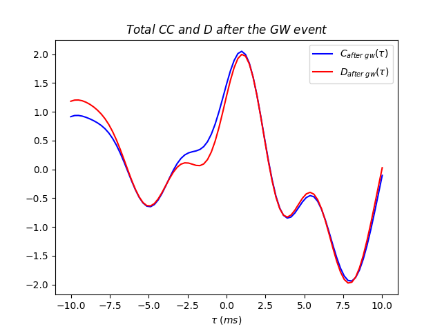 Figure 1
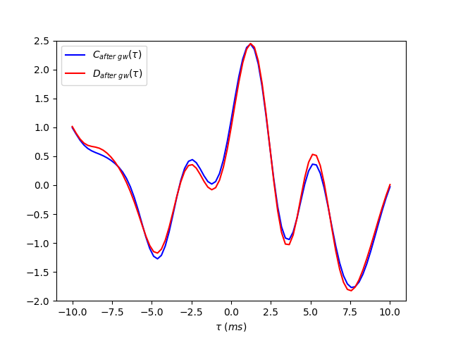 Figure 2
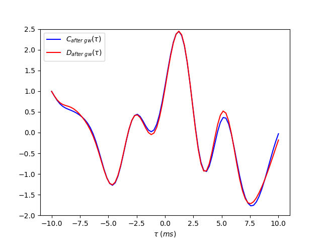 Figure 3
 Figure 4
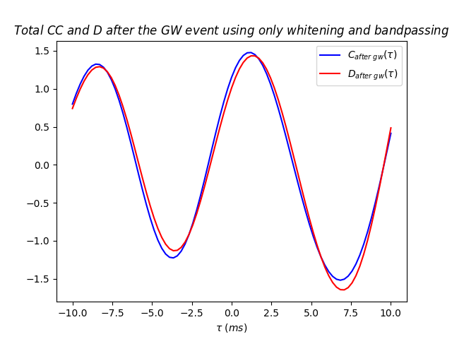 Figure 5
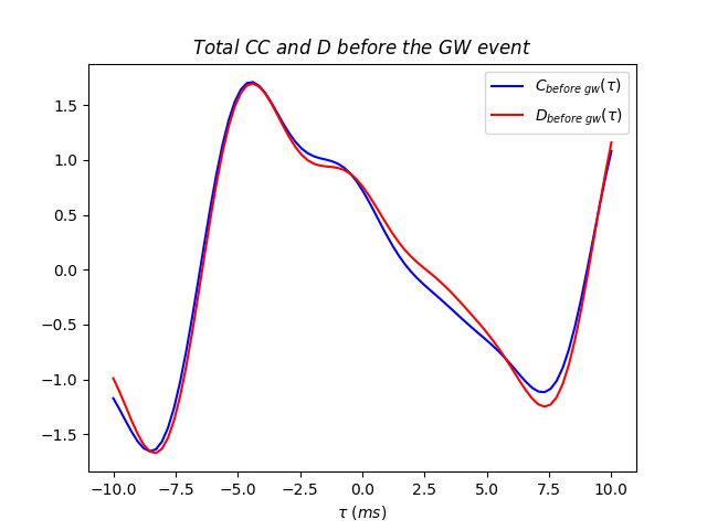 Figure 6
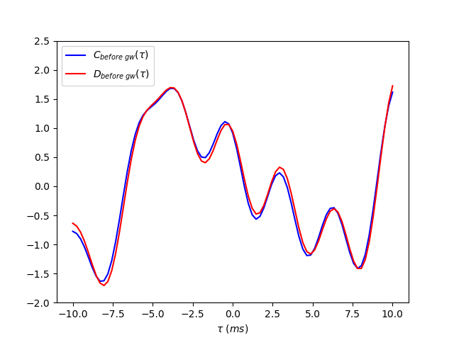 Figure 7
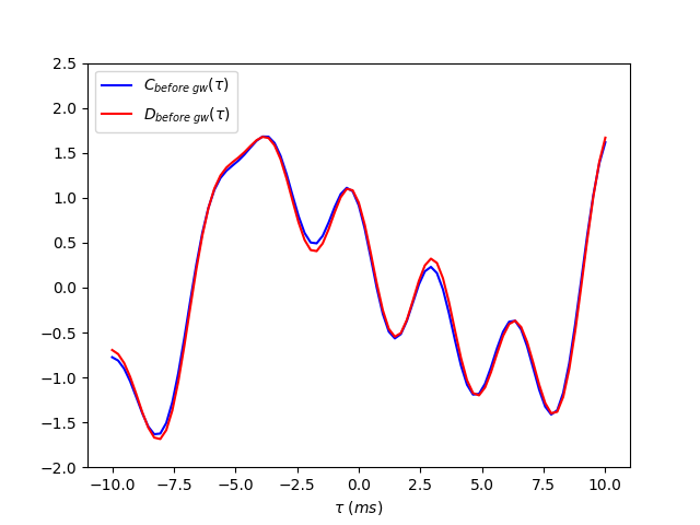 Figure 8
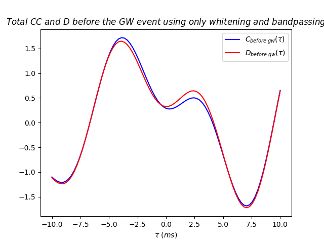 Figure 9
 Figure 10
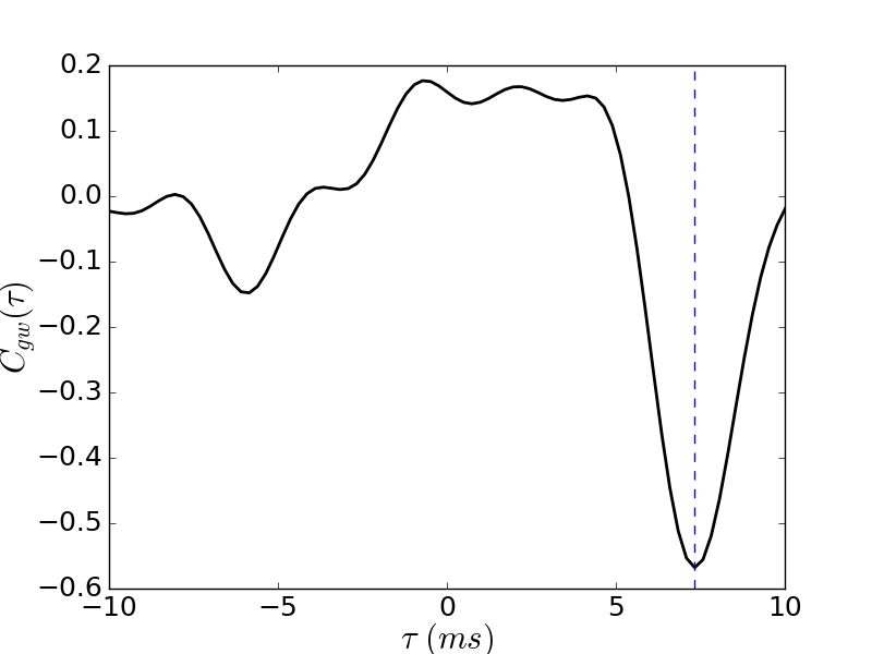 Figure 11
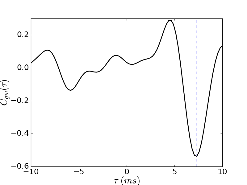 Figure 12
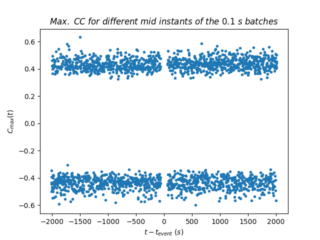 Figure 13
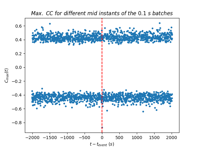 Figure 14
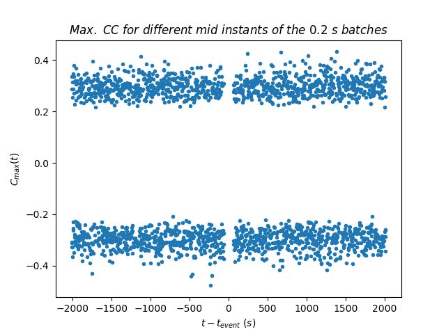 Figure 15
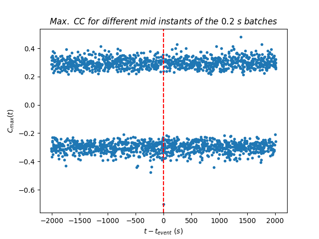 Figure 16
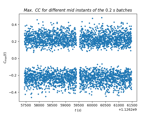 Figure 17
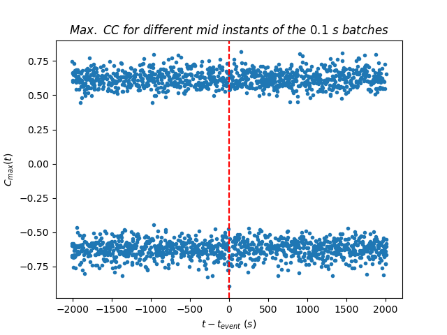 Figure 18
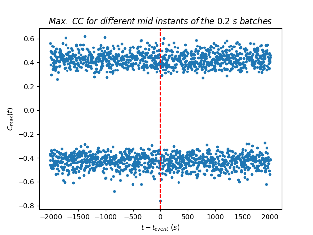 Figure 19
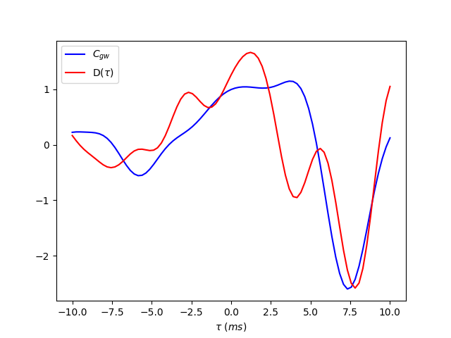 Figure 20
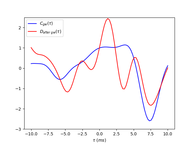 Figure 21
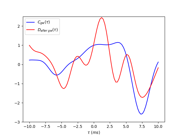 Figure 22
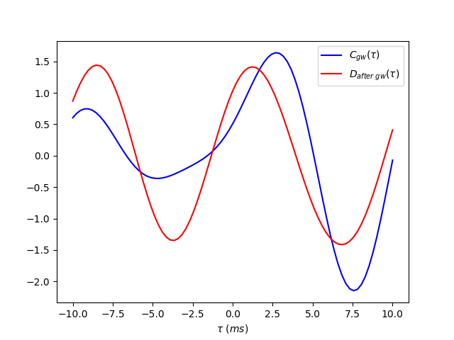 Figure 23
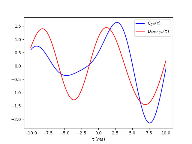 Figure 24
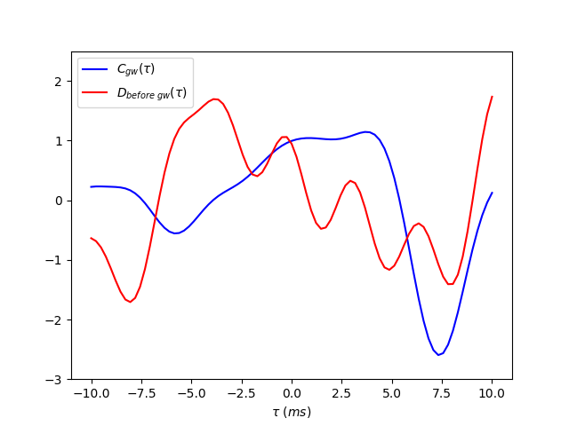 Figure 25
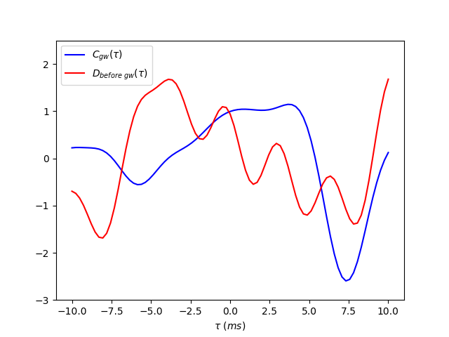 Figure 26
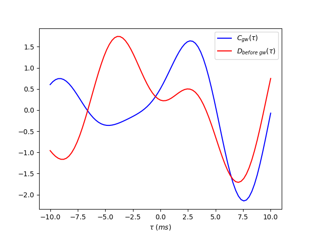 Figure 27
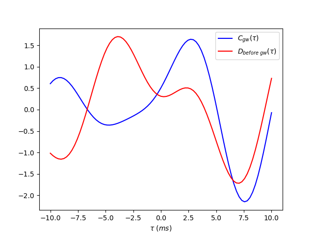 Figure 28
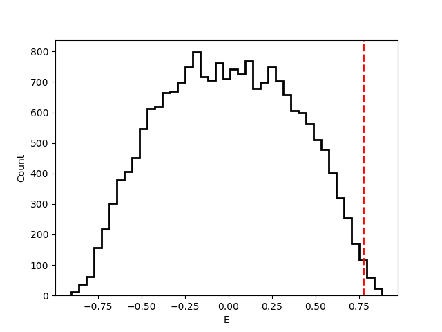 Figure 29
 Figure 30
 Figure 31
 Figure 32
| E(1280, 1988) | E(2108, 4050) | E(1280,1988)(2108, 4050) | |
|---|---|---|---|
| (5 ms, 9 ms) | 0.147 | 0.946 | 0.831 |
| (-10 ms, -6 ms) | -0.976 | 0.969 | -0.523 |
| (-9 ms, -5 ms) | -0.989 | 0.898 | -0.259 |
| (-10 ms, -10 ms) | 0.371 | 0.664 | 0.775 |
| Bandpass range (Hz) | E(-10 ms, 10 ms) |
|---|---|
| 30-50 | 0.813 |
| 50-70 | 0.913 |
| 70-90 | 0.212 |
| 90-110 | 0.996 |
| 110-130 | 0.426 |
| 130-150 | 0.514 |
| E(1280, 2048) | E(2048, 4050) | E(1280, 4050) | |
|---|---|---|---|
| (5 ms, 9 ms) | 0.118 | 0.949 | 0.838 |
| (-9 ms, -5 ms) | -0.954 | 0.932 | -0.743 |
| (-10 ms, -6 ms) | -0.940 | 0.992 | 0.113 |
| (-10 ms, -10 ms) | 0.320 | 0.652 | 0.755 |
Peer Reviews
No public reviews on file for this paper yet. If you reviewed it on a platform where reviews are public (OpenReview, ICLR, NeurIPS, ICML), you can paste yours below so the community can read it here.
Videos
No videos yet. Explain this paper in a talk, walkthrough, or lecture? Add one.
Looking for ancillary signals around GW150914
Rahul Maroju
Sristi Ram Dyuthi
Anumandla Sukrutha
and Shantanu Desai, 11footnotetext: Corresponding author.
Abstract
We replicated the procedure in Liu and Jackson [1], who had found evidence for a low amplitude signal in the vicinity of GW150914. This was based upon the large correlation between the time integral of the Pearson cross-correlation coefficient in the off-source region of GW150914, and the Pearson cross-correlation in a narrow window around GW150914, for the same time lag between the two LIGO detectors as the gravitational wave signal. Our results mostly agree with those in Liu and Jackson [1]. We find the statistical significance of the observed cross-correlation to be about 2.5 . We also used the cross-correlation method to search for short duration signals at all other physical values of the time lag, within this 4096 second time interval, but do not find evidence for any statistically significant events in the off-source region.
1 Introduction
Three and half years ago, there was a watershed moment in astronomy with the detection of gravitational waves, by the LIGO detectors, starting with the first binary black hole merger, viz. GW150914 [2]. Since then, the LIGO-VIRGO collaboration (LVC) has detected a total of seven binary black hole mergers [3, 4, 5, 6, 7] and one binary neutron star merger [8]. These detections (which led to the 2017 Nobel Prize in Physics) have provided a plethora of information about astrophysics, nuclear physics, modified theories of gravity, -process nucleosynthesis, Hubble constant, etc (eg. [9, 10, 11, 12, 13, 14, 15] and references therein). Along with the discoveries, the LIGO open science center (LOSC) has publicly initially released the strain data around each of the detections, and later the full science-mode data from the first two observing runs [16].
Nevertheless, a few groups have still raised a few concerns about some of the LIGO detections [17, 18]. For example, Creswell et al [18] used data from LOSC around GW150914 to point out that the calibration lines and also the residual noise show a peak in the cross-correlation at the same time lag as the original signal. However, at least two groups have been unable to reproduce these results, and therefore dispute these claims [19, 20] (see however [21]). Conversely, some other groups have found evidence for additional signals and anomalies potentially pointing to new Physics [1, 22, 23, 24]. In Refs. [22, 23], the authors have argued for a tentative evidence for echo signals post the merger of the compact objects in both the binary black hole and neutron star events. This work has also received a lot of attention and many groups have tried to reproduce these claims [25, 20, 26]. In Ref. [24], the authors have applied a regularization-based denoising technique to the data around GW150914 and found that the reconstructed waveforms disagree at the high frequency end with the GR-based binary black hole template waveforms. Liu and Jackson [1] (LJ16 hereafter), calculated the Pearson cross-correlation coefficient for data from Hanford and Livingston detectors in the strain data covering 4096 seconds around GW150914. Using this analysis, they have found a tentative evidence (3.2) for a signal 10 minutes before GW150914, lasting for about 45 minutes with the same time lag as GW150914.
Within the LVC, the GW150914 signal was detected by two independent pipelines: one of which involves a matched filtering search from coalescing binaries and the second search involving a model-independent search for short duration signals of any waveform morphology, known as “bursts”. Different burst search algorithms, which look for waveform-agnostic transients in LIGO data do not always detect the same triggers [27]. Therefore, given the importance of gravitational wave detections for physics and astronomy, it is important to verify any concerns about any of the detected events, as well to corroborate any additional signals found by people outside LVC, using independent analysis techniques.
Here, we try to reproduce the claims in LJ16, by trying to mimic their procedure as closely as possible. We also look for short-duration transient signals at all time lags using a simple extension of the method used in LJ16. We note that most recently Nitz et al [28] have carried out a matched filter search (with coalescing binary signals as templates) over the full O1 data and do not find any additional GW signals, beyond those reported. These signals were also not found in the recent re-analysis by the LVC [7]. While this work was in preparation, Nielsen et al. [20] have written a rebuttal countering the claims in Ref. [18] (which is follow-up paper to LJ16), where-in they have also used the Pearson cross-correlation coefficient to examine data around seconds of data around GW150914 signal. However, none of these works have tried to reproduce all the claims in LJ16, or replicated their procedure, therein, which is our goal.
The outline of the paper is as follows. We first briefly recap the results of LJ16 in Sect. 2. We describe the two independent data conditioning steps carried out in Sect. 3. We describe the results from these two steps in Sects. 4 and 5 respectively. We then re-analyze the cross-correlations after removing the best-fit GW signal and these results can be found in Sect. 6. Finally, our estimation of significance using Monte-carlo simulations is discussed in Sect. 7. We conclude in Sect. 8. We have also uploaded our analysis code on github and a web link can be found in Sect. 8.
2 Recap of LJ16
LJ16 downloaded seconds of Hanford and Livingston data (sampled at 16 kHz) around GW150914, starting at GPS time 1126257414. Very simple data conditioning was implemented [29] along the same lines as done by the LVC. The data was band-pass filtered between 50 and 350 Hz using a butterworth filter for the primary analysis. However later, they explored the sensitivity of their significance to different bandwidths. Narrow lines (corresponding to power, calibration and violin mode resonances) were removed in the Fourier domain by clipping the amplitudes to zero power [18]. The final time-series used to search for gravitational waves was then inverse Fourier transformed. A total of 30 seconds of data was excluded at both the ends to avoid boundary artifacts. LJ16 then calculated the function between the time streams of the two LIGO detectors based upon the Pearson cross-correlation coefficient as a function of the time lag (), duration of the signal (). It is defined as follows [1]:
[TABLE]
where and are the time-samples over which Pearson cross-correlation coefficient is calculated; is the Hanford time-series data from () seconds; and is the same for Livingston data from () seconds. We then define for GW150914, which we refer to as as follows
[TABLE]
We note that a similar statistic was previously used as a signal consistency test in the post-processing pipeline for LIGO burst searches during science runs S2, S3, and S4 [30, 31, 32], under the moniker r-statistic [33] or CorrPower [34]. This pairwise cross-correlation posits similarity of the signals (modulo any offsets in calibration). This ansatz is valid for the LIGO detectors, as the 4 km Livingston interferometer is maximally aligned with the Hanford detectors to the extent allowed by Earth’s curvature (modulo a sign flip in one of the detectors, which makes the signals anti-correlated) [35]. For mis-aligned detectors, Pearson cross-correlation cannot be used and needs to be replaced by Rakhmanov-Klimenko cross-correlation or similar variants [36].
In LJ16, cross-correlation has been run in extremely short-duration non-overlapping time windows (0.1 seconds) as well as over data stretches as long as 30 minutes. In Ref. [20], the window duration for calculating cross-correlation was chosen to be 0.2 seconds. To look for weak-amplitude signals, LJ16 introduced the functional , related to the integral of the cross-correlation and is defined as [1]
[TABLE]
where is the duration of the signal. In LJ16, was chosen to be 0.1 seconds, but we consider values of both 0.1 and 0.2 seconds. Note that GW150914 lasted for about 0.2 seconds with frequency sweeping from 35 to 150 Hz over this duration. The main premise in positing the above statistic is that with an increasing window duration, the contribution of noise should decrease, whereas even a weak signal would add up coherently. They also considered the cross-correlation of (from Eq. 2.3) and , (where is calculated over a time interval from to ), which they refer to as and is defined as
[TABLE]
When and were applied to a time stretch of data, 30 minutes before and after the signal (after excluding seconds of data around GW150914), ms. A more precise estimate of the start and stop time of this ancillary signal (in the GW150914 off-source interval) was then obtained by adjusting the start and stop time, as well as by searching in narrow-band filters, until is maximized. The start time of the signal was thereby estimated to be 1280 seconds after the beginning of the starting time stamp (or about 10 minutes before GW150914) and ends 45 minutes later. The statistical significance was estimated by calculating the above statistics for 20,000 different time-shifts with absolute value 10 ms. This estimated statistical significance was about .
3 Data Conditioning of GW150914
For our analysis, we downloaded 4096 seconds of data around GW150914, sampled at 4096 Hz, using version 2 calibration (dubbed v2 and released in October 2016), starting at GPS time 1126257414 (Mon Sep 14 09:16:37 GMT 2015). This start time is about 2048 seconds before the GW150914 signal. This same calibration strain data file was also used in the recent re-analysis in Ref. [20]. Although, the results in LJ16 were obtained using v1 of the calibration, Ref. [20] has shown that the results are not sensitive to the calibration version. Therefore, we stick to v2 of the calibration data for this analysis.
Data conditioning for the event is done in the same way as described in the original GW150914 tutorial on the LOSC webpage https://www.gw-openscience.org/s/events/GW150914/GW150914_tutorial.html. Note that on this tutorial webpage, it has been shown the signal is visible using two independent data conditioning procedures. The first procedure involves whitening in the frequency domain followed by band pass filtering (in the time-domain using a butterworth filter). Whitening in the frequency domain is mathematically equivalent to dividing the input data in the Fourier domain by its amplitude spectral density. This whitened frequency domain data is then transformed back to the time domain, which is then used for GW analysis. Alternately, the signal is also visible from the same band-pass butterworth filter, followed by application of IIR notch filtering in the time domain to get rid of various lines. As mentioned earlier, this signal was seen by both the burst and compact binary coalescence-based matched filtering search pipelines, which look for inspiral and merger of compact stellar remnants, also known as “CBC” within the LVC [37, 38]. The burst search was done using two pipelines, coherent Waveburst (cWB) [39] and also omicron-LALInference-Bursts [40]. The cWB algorithm uses a linear predictive error filter, which is equivalent to whitened time series [39]. The CBC search was also carried out using two pipelines, called PyCBC [41] and GstLAL [42]. Both these pipelines employ a whitening filter in the data conditioning steps.
As discussed in Sect. 2, LJ16 have applied a band-pass window followed by notch windows, obtained using clipping in the frequency domain. We also note that in the Block-Normal burst search pipeline [43], which was used until S5 [44], data conditioning consisted of all three steps (band-passing, whitening and line removal) [45]. In some other pipelines, the data has been whitened using a running median [46].
Therefore, there is no unique data conditioning procedure followed by the different GW search algorithms. Here, we present our results using both band-pass and notch filtering (for line removal), as well as using band-pass and whitening. Ref. [20] have also done their analysis using notch filtering as well as whitening. The code for implementing these steps has been described on the aforementioned LOSC webpage. We now briefly describe both these steps.
We first apply FFT to the full 4096 seconds of data. We then apply a bandpass filter between 50 Hz and 350 Hz to suppress the low-frequency noise (mainly due to seismic activity) and high frequency noise (mainly due to quantum noise) [47]. The noise floor shows a steep rise in this frequency range [48], and hence the signal is always band-passed in this intermediate frequency range to search for astrophysical signals. The band-passing is implemented using a linear butterworth filter. The LIGO noise spectrum also contains a number of lines in the frequency domain due to mechanical resonances, power line harmonics, etc [47]. These have been removed using IIR based time-domain notch filtering, following the algorithm on the above webpage. The list of lines for which the notch filter has been applied include 14, 34.7, 35.3, 36.7, 37.3, 40.95, 60.0, 120.0, 179.99, 304.99, 331.49, 510.02, 1009.99 Hz respectively. The same lines have also been notch-filtered in a follow-up paper by Creswell et al. [18]. Results from this data conditioning procedure are described in Sect. 4.
For our second set of results, instead of notch-filtering, we applied a whitening filter, by dividing by the noise spectrum in the frequency domain using the same code as mentioned on the above LOSC tutorial website.
4 Results from band-passing and notch filtering
Here, we describe our results after the application of band-pass filtering and notching. The corresponding results after the application of the whitening filter, instead of the notch filter shall be described in Sect. 5.
Similar to LJ16, we exclude the first and last 30 seconds of the data. Using this data, we first calculate as a function of the time lag () between the two LIGO detectors in a 0.2 second window around GW150914 corresponding to the GPS time of 1126259462.42 (Sep 14 09:50:45). Since we have downsampled the data to 4 kHz, the minimum resolution in the time lags we can have is 0.246 milliseconds. This plot can be found in Fig. 1 and is similar to Fig. 1 of LJ16 or the corresponding plot in Fig. [20]. One can see a sharp dip for a time lag close to 7.33 ms corresponding to the signal. Note that unlike LJ16, we do not find a minimum value of closer to 6.9 ms. The peak absolute value of is at ms, closer to the value found in Ref. [20]. The uncertainty in the peak time is about 0.246 milliseconds, which is limited by the downsampled frequency of 4 kHz. Similar to LJ16, we then calculated (from ) for a long time stretch of data spanning 30 minutes before and after the GW signal, after excluding the data within seconds around GW150914. We then overlay this along with for seconds around GW150914. Note that for this purpose similar to LJ16, both and have been rescaled, so that they have a mean value of zero and a rms value of one. To calculate , one needs to integrate over a window duration. For the calculation of , we calculated in both 0.1 and 0.2 second windows. These plots for and using both the windows can be found in Figs. 2 and 3. We find roughly the same behaviour as in Fig. 1 of LJ16. In the panels showing the data after GW150914, we find a near-maximal correlation (similar to LJ16) between and at the same time lag as GW150914. However, we also find a similar correlation at the opposite end for between -7 and -10 ms. Therefore, it is not immediately obvious if the strong correlation between and at the same time lag as GW150914 is pointing to a post-merger signal.
As an extension of this technique, we then look for additional short duration signals lasting 0.1 and 0.2 seconds using the cross-correlation method, which may appear at arbitrary time lags. Furthermore, if there is a persistent long-duration signal, then should have the same value across many 0.1/0.2 second chunks. For this purpose, we calculated the cross-correlation in each 0.1/0.2 second chunk for the entire 4096 seconds of LIGO data, for time lags ranging from -10 to 10 milliseconds. These plots can be found in Fig. 3 and Fig. 4. The maximum (absolute) value of is seen at the peak of GW150914. We do not find any values of as large as that for GW150914 at any other times. For the 0.1 second window, the maximum cross correlation in the off-source region has a value of 0.63 at the GPS time of 1126257962.4, about 548 seconds from the start of the time series or 1500 seconds before GW150914. For the 0.2 second window, the maximum absolute cross correlation in the off-source region equal to -0.47 occurs at the GPS time of 1126259229.4, about 1815 seconds from the start of our time series, or 233 seconds before GW150914. The maximum (absolute) values of at the peak of GW150914 are -0.7 and -0.87 for the 0.2 and 0.1 second windows respectively.
Therefore, with this data conditioning procedure, we roughly agree with the results in LJ16, although we also find a strong correlation between and for time lags close to -10 ms, which is far from the time lag seen for GW150914. However, when we scanned the full 4096 seconds of data around GW150914, we do not find any other value of calculated in small duration windows, whose absolute value is as large as GW150914, for both the windows.
4.1 Correlation between and
To further pin down the exact start and end time of the signal, LJ16 calculated (cf. 2.5) by calculating the cross-correlation between and . They find that is maximized, when the signal starts at 1280 seconds and ends at 4050 seconds from the start of the downloaded data segment. We calculated the values of for the same starting and ending times as LJ16 from 1280 to 4050 seconds. Note however that unlike LJ16, we have excluded the data within seconds around GW150914, for evaluating , in order to avoid any bias from the GW signal in the final value for 222LJ16 found that excluding the data around GW150914 for the purpose of calculating , does not change the results in Section III B if their paper (H. Liu, private communication).. Therefore, instead of , , and , we evaluated , , and . Given the similarity in the trends of and for time lags close to -10 ms, we also checked the value of for ms and ms. These values of can be found in Table 1. Similar to LJ16, we find that is largest for (5,9) ms, and for (-10,10) ms, is largest for and , even after excluding 60 seconds around GW150914. Therefore, our results for are broadly in agreement with those in LJ16, even after excluding seconds of data around GW150914 signal. However, we also find a value for very close to one for ms. If there was an external ancillary post-merger signal at the same time lag as GW150914, then we cannot think of any apriori reason why should be close to one for a time lag close to -10 ms.
We then repeat the test carried out in LJ16 by band-passing the data into contiguous 20 Hz bands between 30 Hz and 150 Hz. These values for in different bands can be found in Table 2. Our results agree with Table II in LJ16. We also find that the correlations in 50-70 Hz and 90-110 Hz are very close to 1.
Therefore, to summarize, our results for broadly agree with those in LJ16, for the same time lag as GW150914 (7.5 ms). But we also find a large value for at time lags between and ms.
5 Results after band-pass filtering and whitening
We now go through the same exercise as in Sect. 4, after skipping the notch filtering step, but replacing it by whitening the data. We first calculate the cross-correlation in a second window around GW150914 , and the resulting figure can be found in Fig. 6. Again, we see a peak at around 7.33 milliseconds. We then calculate and for the same time window as in Figs. 2 and 3. These plots for 0.1 and 0.2 second signal durations can be found in Figs. 7 and 8. Again, the qualitative trends are similar to those in Figs. 2 and 3, and similar to LJ16, we see a strong correlation between and at the same time lag as GW150914, for a 30 minute stretch of data after GW150914. However, for the same data, we also notice a correlation between and for between -7.5 and -10.0 ms.
Finally, the values of in 0.1 and 0.2 second chunks are shown in Figs. 9 and 10. We do not find any other time interval with a value of as large as that of GW150914. In the off-source region and for a 0.1 second time interval, the maximum (absolute) cross correlation is about -0.82 and occurs at a GPS time of 1126259188.7, which is about 1774 seconds from the start of the time-series, or 274 seconds before GW150914. For the 0.2 second window, the maximum (absolute) cross correlation is about -0.68 and occurs at the GPS time of 1126258623.6, which is about 1209 seconds from the start of the time series, or 839 seconds before GW150914. The maximum (absolute) values of at the peak of GW150914 are -0.76 and -0.82 for the 0.2 and 0.1 second windows respectively.
Therefore, even after the application of a whitening filter (instead of notch filter) as part of the data conditioning step, the trends in and are in agreement with those in LJ16, as well as our previous results discussed in Sect. 4. Based upon the values of in 0.1 and 0.2 second windows, we do not find evidence for any additional short duration signals in the off-source region of GW150914.
6 Cross-correlations after removing the GW signal
In Sections 4 and 5, we have calculated the cross-correlation between and , after removing 60 seconds of data around GW150914 in the calculation of . Here, we redo the cross-correlation after including these 60 seconds, but after subtracting the gravitational wave signal around GW150914. For this purpose, we subtracted the matched filter template from the filtered data in a 0.45 seconds window starting from GPS time 1126259462 (Sep 14 09:50:45 GMT 2015) 333For this analysis, we directly used the residuals provided by the LOSC, which are available at https://www.gw-openscience.org/s/events/GW150914/P150914/fig1-residual-H.txt and fig1-residual-L.txt, so that the full datastream used in the calculation of is consistent with noise. We show the trends for (after using this data with the GW signal subtracted) in a time window from 1280 to 4050 seconds, along with in Fig. 11. Similar to before, we see a strong correlation between and .
We then repeat the same exercise as in Sect. 4.1 and calculate in the same time windows using this signal-subtracted data around GW150914. These results can be found in Table 3. The results are the same as in Table 1. We still see a value for close to one for ms and ms.
7 Estimation of significance
To estimate the statistical significance for our values of in Sections 4.1 and 6, we time-shift the data from one of the detectors using unphysical time lags, in order to generate Monte-Carlo simulations for a pure noise floor. A similar procedure is usually used to estimate the significance of all thw GW detections by the LVC collaboration (cf. Ref. [2] for GW150914), and was also used by LJ16 to estimate the significance of their estimated values of .
Here, we consider the Hanford data from 1280 to 4050 seconds. We then analyze the Livingston data with the same duration, but time-shifted with respect to Hanford data from () seconds in 20,000 steps.444Note that in LJ16 to estimate the statistical significance, only one second of Hanford/Livingston data separated by unphysical time lags has been used (H. Liu, private communication). For each value of this time-shifted pair of data, we calculate for ms. Each is cross-correlated with to evaluate . Each value of using this combination of data with unphysical time lags, can be considered as the value for “null-stream” data with no signal and any value close to one, can only be because of a statistical fluctuation. The observed values of for each of these realizations can be found in Fig. 12.
The number of realizations, which exceed our observed value of equal to 0.775 (cf. Sect. 4.1) is equal to 126 out of 20,000, corresponding to a false alarm probability (FAP) of or a significance of 2.5. The number of realizations for which we get a value of greater then 0.755 (which we get after including the subtracting the GW signal around GW150914, as outlined in Sect. 6) is 192 out of 20,000, for a false alarm probability (FAP) of or a significance of 2.34. Finally, we get a value of , greater than that obtained in LJ16 (viz. 0.84) for 22 out of 20,000 realizations, for a FAP of corresponding to a significance of 3.06. This significance is about the same as found in LJ16.
8 Conclusions
We replicate the procedure in LJ16 [1], to see if we can independently corroborate their claim of a long duration low-amplitude signal at in the vicinity of GW150914 at the same time lag (as GW150914). We implemented two different data conditioning procedures for data within 2048 seconds of GW150914 (which lasted for about 0.2 seconds from 35 to 150 Hz). The only difference with respect to the analysis in LJ16 is that we have used version 2 of the calibrated strain data and applied notch filtering in the time domain, instead of clipping in the frequency domain as in LJ16. Similar to LJ16, we calculated the Pearson cross-correlation coefficient (), and also its integral for 0.1 and 0.2 second windows across the full 2048 seconds of data. LJ16 had found that in this off-source region is maximally correlated with for the same time lag as GW150914, where is the Pearson cross-correlation coefficient for a time-window around GW150914. They showed that this ancillary signal lasted between 1280 and 4050 seconds, where the zero point corresponds to 2048 seconds before GW150914. We roughly find the same trends in the behaviour of and , using both the data conditioning procedures. Similar to LJ16, we find a strong correlation in and at the same time lag as GW150914 (around 7.5 ms) in a 30-minute window after GW150914. We then reanalyzed the cross-correlation between and , after including the full data stream, but after removing the best-fit template around the GW signal. We find that the values of for time lags close to 7.5 ms is about the same as before. We also the statistical significance of obtaining a value greater than our observed cross-correlation to be about , which is roughly comparable to the significance of found in LJ16.
As an extension of this method, we also evaluated the cross-correlation coefficient in non-overlapping 0.1/0.2 second windows in order to discern the existence of any other short duration signal in the off-source region, for all physical time lags. We do not find any other data stretch, which shows a value of in this region, which could be deemed statistically significant.
We have made available our Python scripts containing all the codes to reproduce the results at https://github.com/RahulMaroju/GW150914-analysis
Acknowledgments
This research has made use of data, software and/or web tools obtained from the Gravitational Wave Open Science Center (https://www.gw-openscience.org), a service of LIGO Laboratory, the LIGO Scientific Collaboration and the Virgo Collaboration. LIGO is funded by the U.S. National Science Foundation. Virgo is funded by the French Centre National de Recherche Scientifique (CNRS), the Italian Istituto Nazionale della Fisica Nucleare (INFN) and the Dutch Nikhef, with contributions by Polish and Hungarian institutes. We thank Hao Liu for explaining in detail all the technical details of LJ16. We are grateful to Soumya Mohanty for the comments on the manuscript and to Malik Rakhmanov for helpful correspondence.
The reference list from the paper itself. Each links out to its DOI / PubMed record.
- 1[1] H. Liu and A. D. Jackson, Possible associated signal with GW 150914 in the LIGO data , JCAP 1610 (2016) 014 [ 1609.08346 ]. · doi ↗
- 2[2] Virgo, LIGO Scientific collaboration, Observation of Gravitational Waves from a Binary Black Hole Merger , Phys. Rev. Lett. 116 (2016) 061102 [ 1602.03837 ]. · doi ↗
- 3[3] Virgo, LIGO Scientific collaboration, Binary Black Hole Mergers in the first Advanced LIGO Observing Run , Phys. Rev. X 6 (2016) 041015 [ 1606.04856 ]. · doi ↗
- 4[4] VIRGO, LIGO Scientific collaboration, GW 170104: Observation of a 50-Solar-Mass Binary Black Hole Coalescence at Redshift 0.2 , Phys. Rev. Lett. 118 (2017) 221101 [ 1706.01812 ]. · doi ↗
- 5[5] Virgo, LIGO Scientific collaboration, GW 170814: A Three-Detector Observation of Gravitational Waves from a Binary Black Hole Coalescence , Phys. Rev. Lett. 119 (2017) 141101 [ 1709.09660 ]. · doi ↗
- 6[6] Virgo, LIGO Scientific collaboration, GW 170608: Observation of a 19-solar-mass Binary Black Hole Coalescence , Astrophys. J. 851 (2017) L 35 [ 1711.05578 ]. · doi ↗
- 7[7] LIGO Scientific, Virgo collaboration, GWTC-1: A Gravitational-Wave Transient Catalog of Compact Binary Mergers Observed by LIGO and Virgo during the First and Second Observing Runs , 1811.12907 .
- 8[8] Virgo, LIGO Scientific collaboration, GW 170817: Observation of Gravitational Waves from a Binary Neutron Star Inspiral , Phys. Rev. Lett. 119 (2017) 161101 [ 1710.05832 ]. · doi ↗