TL;DR
This paper extends the model-X knockoffs method by relaxing the assumption of knowing the exact covariate distribution, instead allowing for a parametric model with many parameters, while maintaining false discovery rate control.
Contribution
It shows that knockoffs guarantees hold when the covariate distribution is known only up to a parametric model, using conditioning on sufficient statistics.
Findings
Maintains FDR control under weaker assumptions.
Effective in Gaussian models with conditioning on sufficient statistics.
Simulations demonstrate robustness of the new approach.
Abstract
The recent paper Cand\`es et al. (2018) introduced model-X knockoffs, a method for variable selection that provably and non-asymptotically controls the false discovery rate with no restrictions or assumptions on the dimensionality of the data or the conditional distribution of the response given the covariates. The one requirement for the procedure is that the covariate samples are drawn independently and identically from a precisely-known (but arbitrary) distribution. The present paper shows that the exact same guarantees can be made without knowing the covariate distribution fully, but instead knowing it only up to a parametric model with as many as parameters, where is the dimension and is the number of covariate samples (which may exceed the usual sample size of labeled samples when unlabeled samples are also available). The key is to treat the…
Click any figure to enlarge with its caption.
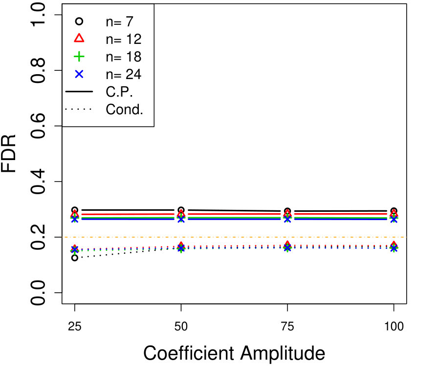 Figure 1
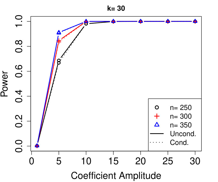 Figure 2
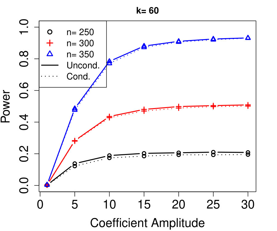 Figure 3
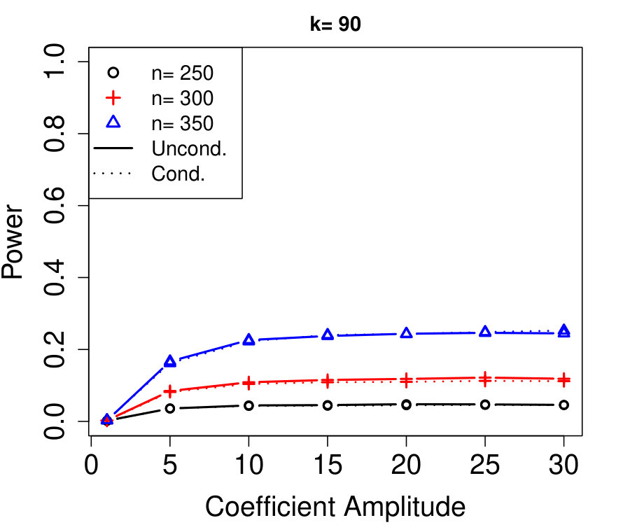 Figure 4
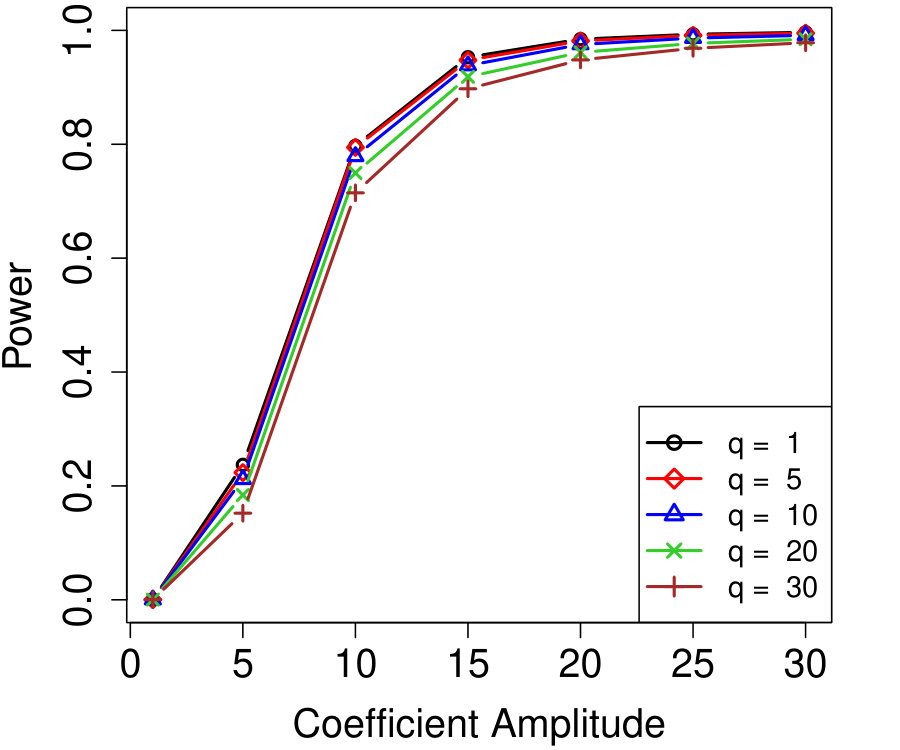 Figure 5
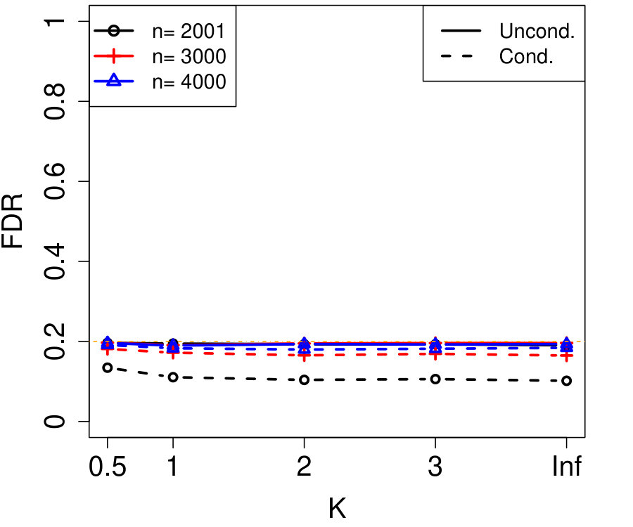 Figure 6
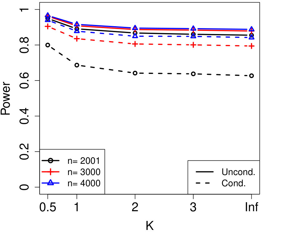 Figure 7
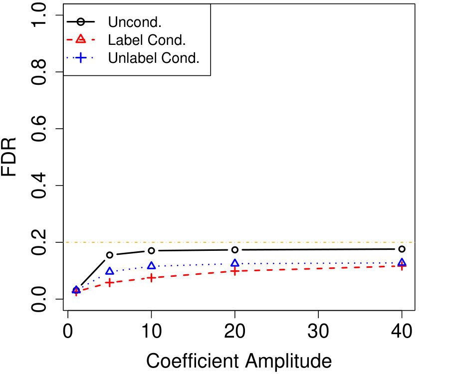 Figure 8
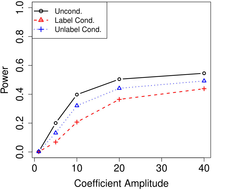 Figure 9
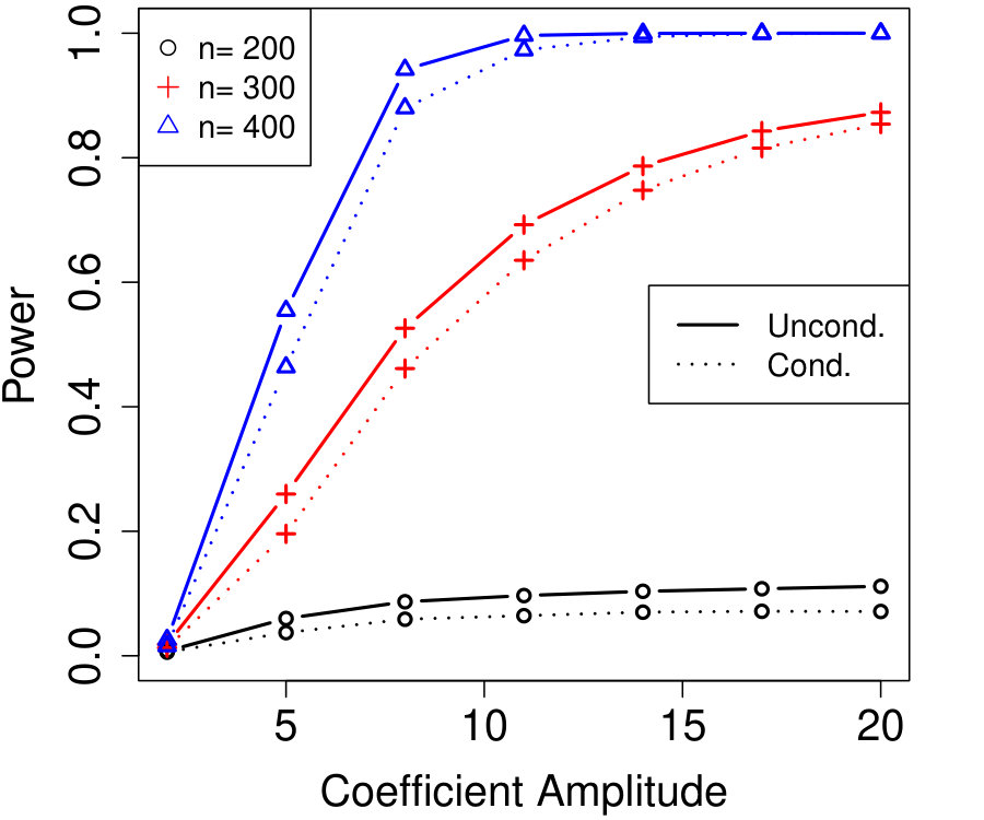 Figure 10
 Figure 11
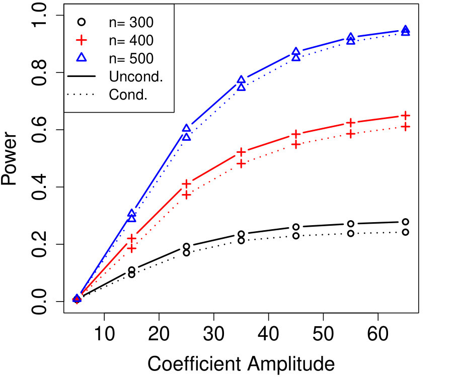 Figure 12
 Figure 13
 Figure 14
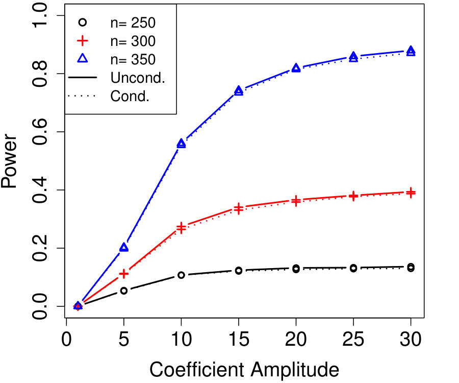 Figure 15
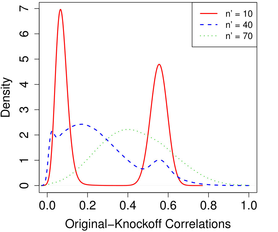 Figure 16
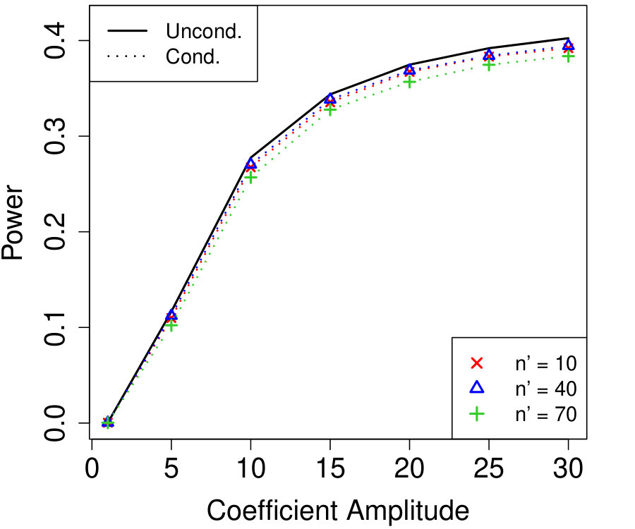 Figure 17
 Figure 18
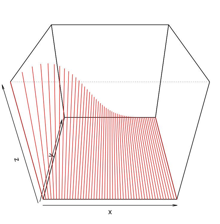 Figure 19
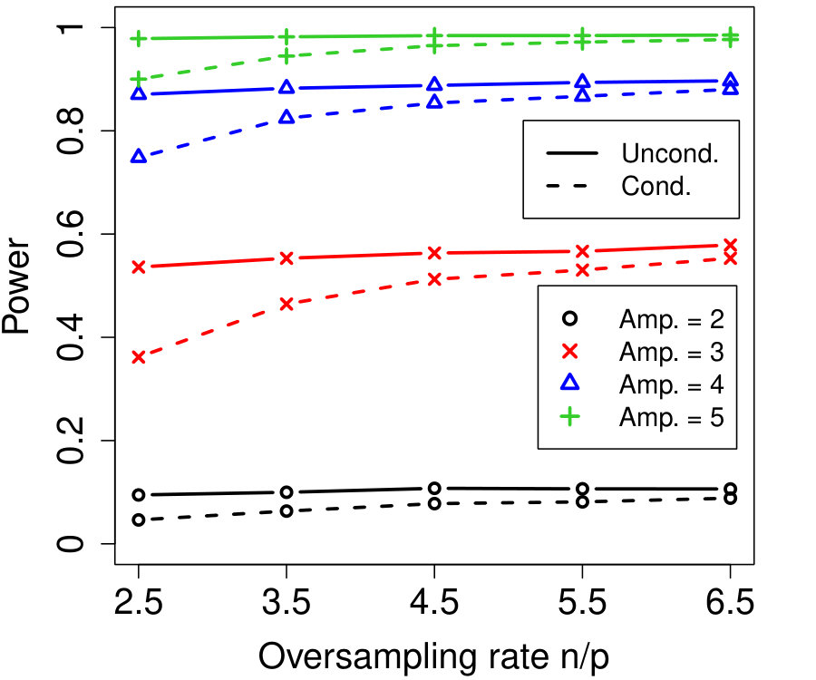 Figure 20
 Figure 21
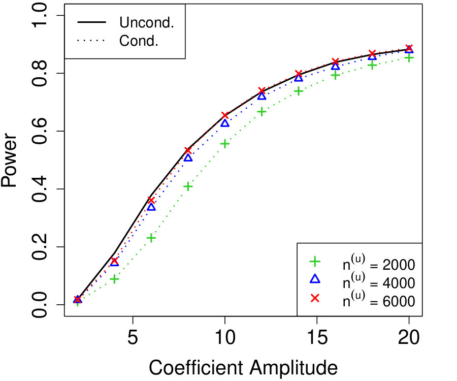 Figure 22
 Figure 23
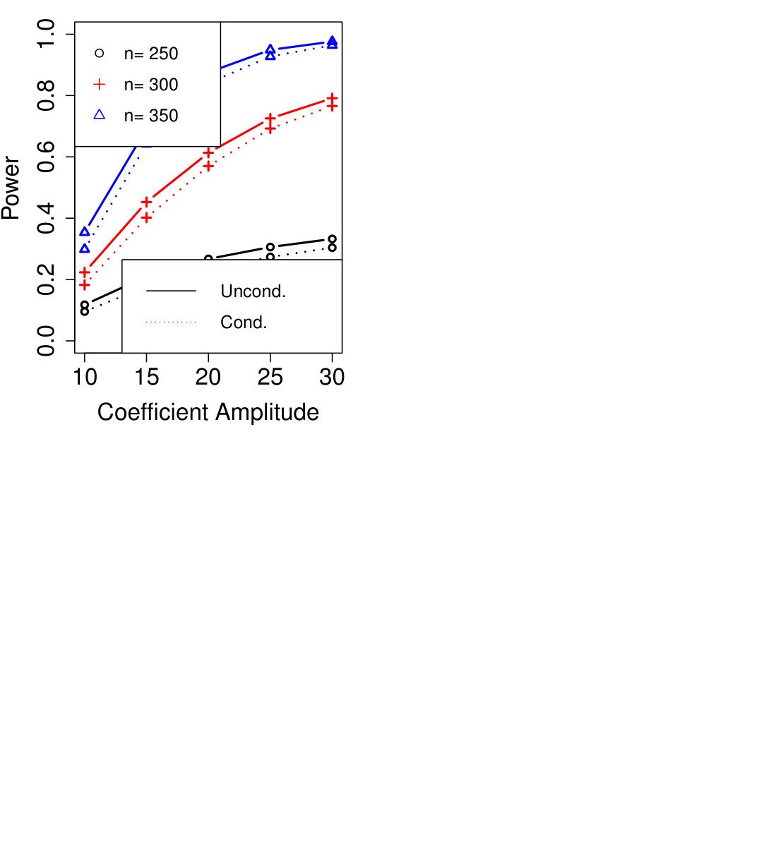 Figure 24
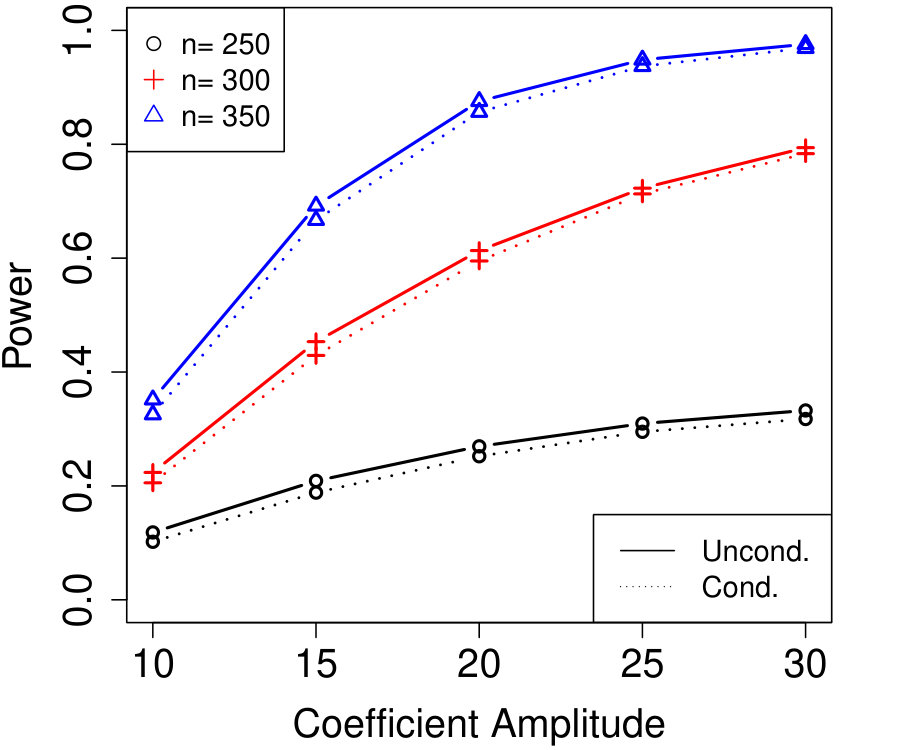 Figure 25
 Figure 26
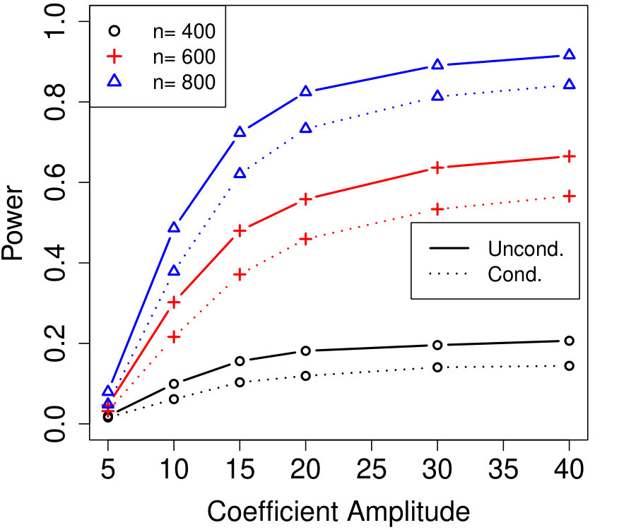 Figure 27
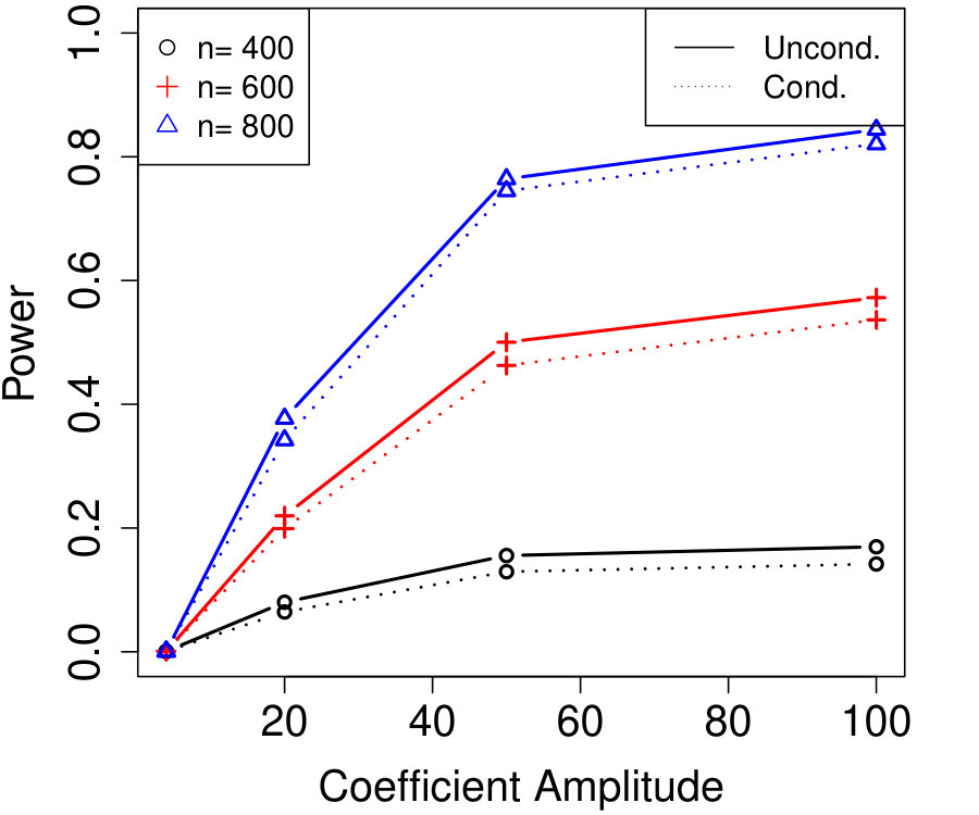 Figure 28
 Figure 29
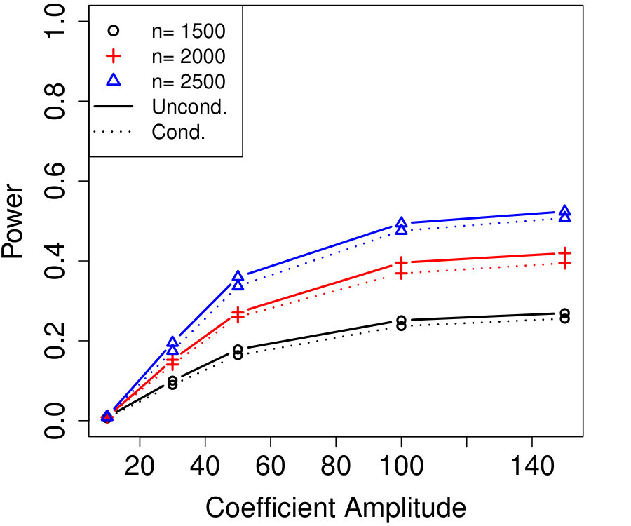 Figure 30
 Figure 31
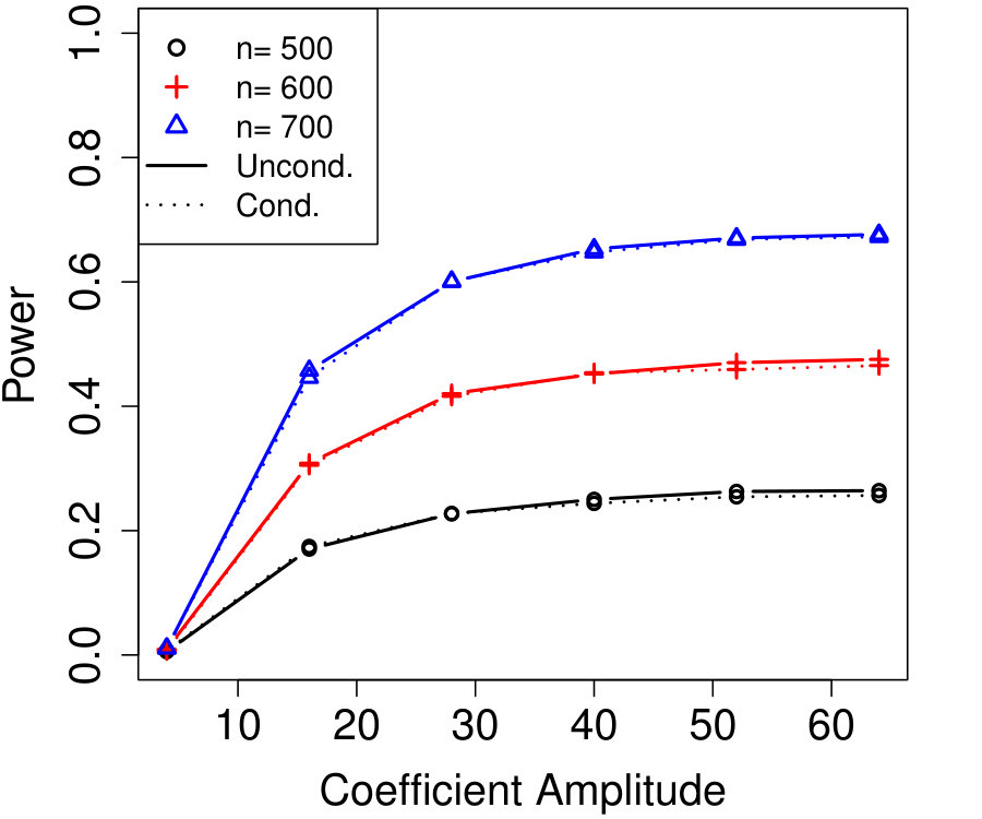 Figure 32
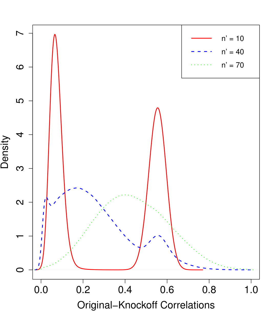 Figure 33
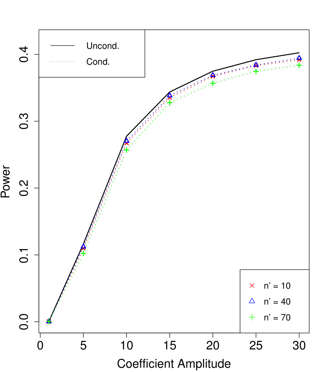 Figure 34
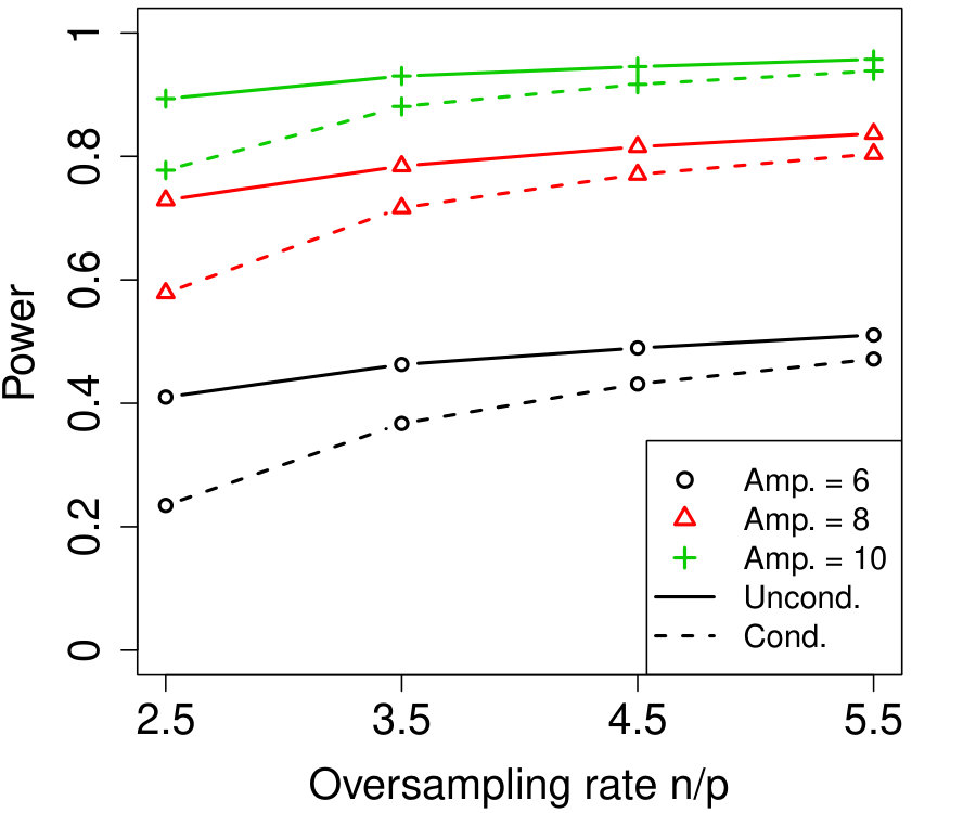 Figure 35
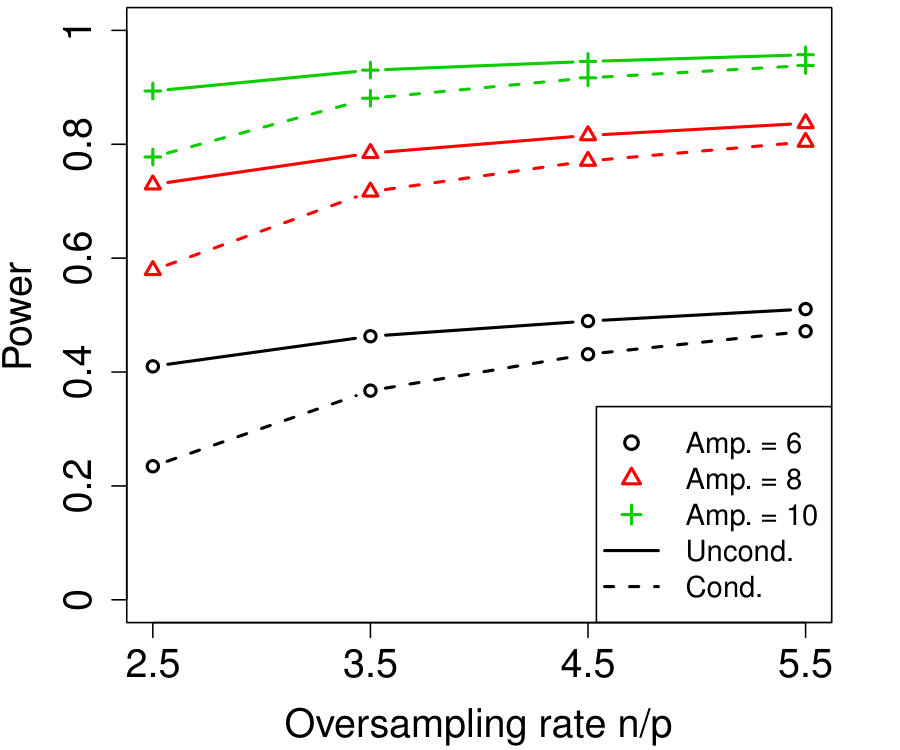 Figure 36
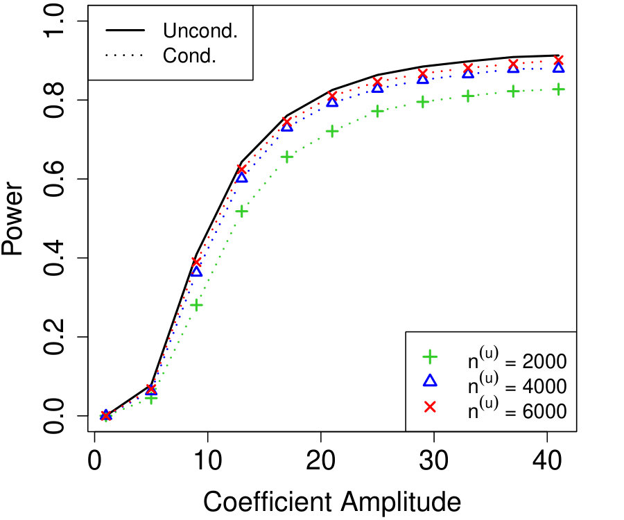 Figure 37
 Figure 38
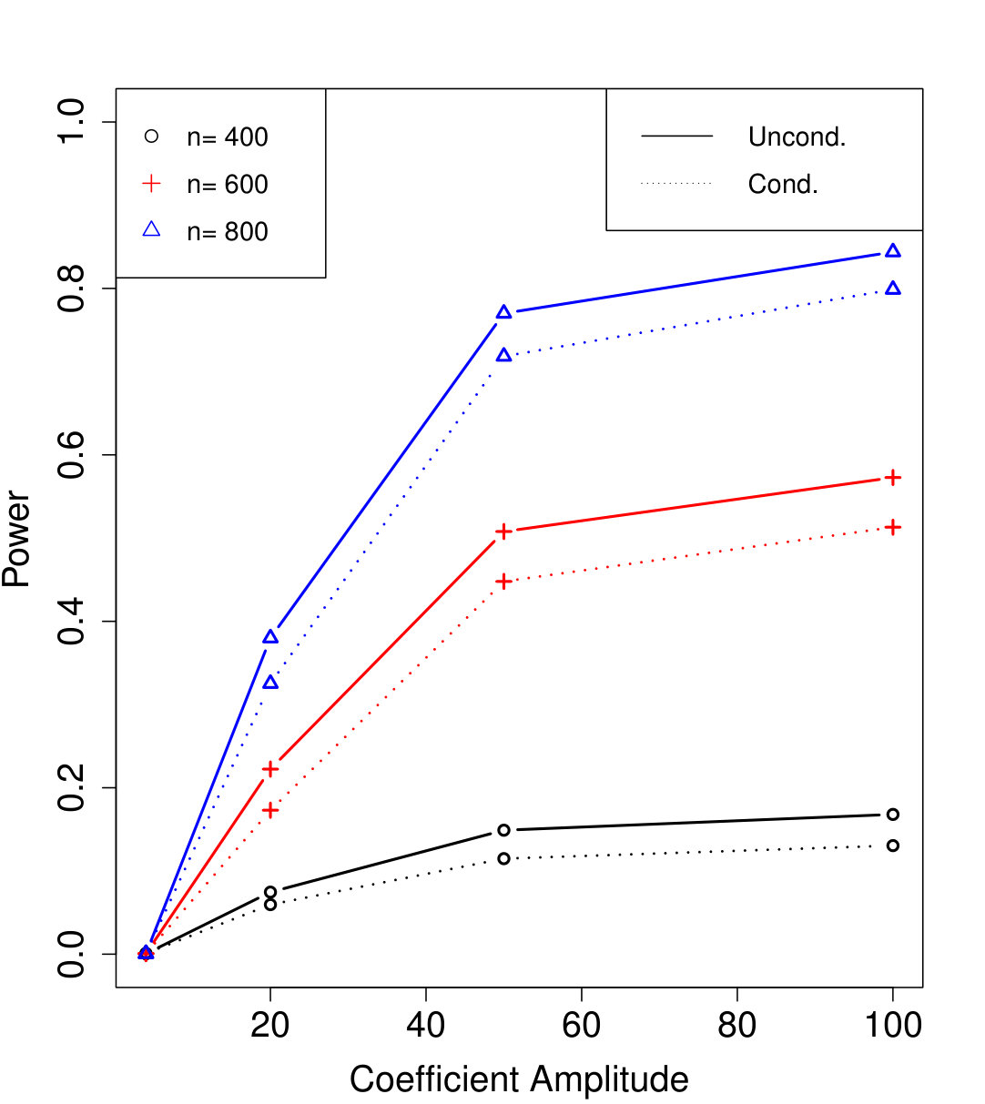 Figure 39
| Model for | Model for | |||
| Fixed-X | parameters333In the exceptional case of Gaussian linear regression, parameters are allowed.,444Except for Gaussian linear regression, fixed-X inferential guarantees are only asymptotic. | arbitrary | ||
| Model-X (Candès et al.,, 2018) | arbitrary | parameters | ||
| Model-X (this paper) | arbitrary | parameters |
Peer Reviews
No public reviews on file for this paper yet. If you reviewed it on a platform where reviews are public (OpenReview, ICLR, NeurIPS, ICML), you can paste yours below so the community can read it here.
Code & Models
Videos
No videos yet. Explain this paper in a talk, walkthrough, or lecture? Add one.
Relaxing the Assumptions of Knockoffs by Conditioning
Dongming Huang
Lucas Janson
Abstract
The recent paper Candès et al., (2018) introduced model-X knockoffs, a method for variable selection that provably and non-asymptotically controls the false discovery rate with no restrictions or assumptions on the dimensionality of the data or the conditional distribution of the response given the covariates. The one requirement for the procedure is that the covariate samples are drawn independently and identically from a precisely-known (but arbitrary) distribution. The present paper shows that the exact same guarantees can be made without knowing the covariate distribution fully, but instead knowing it only up to a parametric model with as many as parameters, where is the dimension and is the number of covariate samples (which may exceed the usual sample size of labeled samples when unlabeled samples are also available). The key is to treat the covariates as if they are drawn conditionally on their observed value for a sufficient statistic of the model. Although this idea is simple, even in Gaussian models conditioning on a sufficient statistic leads to a distribution supported on a set of zero Lebesgue measure, requiring techniques from topological measure theory to establish valid algorithms. We demonstrate how to do this for three models of interest, with simulations showing the new approach remains powerful under the weaker assumptions.
Keywords. High-dimensional inference, knockoffs, model-X, sufficient statistic, false discovery rate (FDR), topological measure, graphical model
1 Introduction
1.1 Problem statement
In this paper we consider random variables where is a response or outcome variable, each is a potential explanatory variable (also known as a covariate or feature) and is the dimensionality, or number of covariates. For instance, could be the binary indicator of whether a patient has a disease or not, and could be the number of minor alleles at a specific location (indexed by ) on the genome, also known as a single nucleotide polymorphism (SNP). A common question of interest is which of the are important for determining , with importance defined in terms of conditional independence. That is, is considered unimportant (or null) if
[TABLE]
where ; stated another way, is unimportant exactly when ’s conditional distribution does not depend on . Denote by the set of all such that is unimportant. As discussed in Candès et al., (2018), under very mild conditions the complement of the set of unimportant variables, i.e., the important (or non-null) variables, constitutes the Markov blanket of , namely, the unique smallest set such that Y\mathchoice{\mathrel{\hbox to0.0pt{\displaystyle\perp\hss}\mkern 2.0mu{\displaystyle\perp}}}{\mathrel{\hbox to0.0pt{\textstyle\perp\hss}\mkern 2.0mu{\textstyle\perp}}}{\mathrel{\hbox to0.0pt{\scriptstyle\perp\hss}\mkern 2.0mu{\scriptstyle\perp}}}{\mathrel{\hbox to0.0pt{\scriptscriptstyle\perp\hss}\mkern 2.0mu{\scriptscriptstyle\perp}}}X_{S}\mid X_{\text{-}S}. Note that when follows a generalized linear model (GLM) with no redundant covariates, the set of important variables exactly equals the set of variables with nonzero coefficients, as usual (Candès et al.,, 2018).
In our search for the Markov blanket we usually cannot possibly hope for perfect recovery, so we instead attempt to maximize the number of important variables discovered while probabilistically controlling the number of false discoveries. In this paper, as with most others in the knockoffs literature,111Janson and Su, (2016) show how the last step of knockoffs can easily be modified to control other error rates such as the -familywise error rate. we consider the false discovery rate (FDR) (Benjamini and Hochberg,, 1995), defined for a (random) selected subset of variables as
[TABLE]
i.e., the expected fraction of discoveries that are not in the Markov blanket (false discoveries), where we use the convention that . Controlling the FDR at, say, is powerful as compared to controlling more classical error rates like the familywise error rate, while still being interpretable, allowing a statistician to report a conclusion such as “here is a set of covariates , 90% of which I expect to be important.”
1.2 Our contribution
In our discussion of approaches to this problem, we will draw on a fundamental decomposition of the joint distribution of into the product of the conditional distribution of and the joint distribution of . The canonical approach to inference, which we refer to as the ‘fixed-X’ approach, assumes is a member of a parametric family of conditional distributions (e.g., a GLM), while placing weak or no assumptions on . In fact, the fixed-X approach usually treats the observed values of for as fixed; that is, it performs inference conditionally on the observed values of in the data, which also allows the covariate rows to be drawn from different distributions or even be deterministic (fixed). The approach proposed in Candès et al., (2018), referred to therein as the ‘model-X’ approach, assumes the observations and places no restrictions on but assumes it is known exactly, while assuming nothing about . So, to summarize slightly imprecisely, the canonical, fixed-X approach to inference places all assumptions on and none on , while the model-X approach does the opposite by placing all assumptions on and none on .
Note that both and are exponentially complex in : in the simple case where each element of is categorical with categories, i.e., , it is easily seen that a fully general model for has free parameters while has only slightly fewer with . So both fixed-X and model-X approaches astronomically reduce an exponentially large (in ) space of distributions in order to make inference feasible, highlighting the importance of robustness, assumption-checking, and domain knowledge for justifying the resulting inference; see Janson, (2017, Chapter 1) for a detailed discussion of the role of fixed-X and model-X222Therein referred to as ‘model-based’ and ‘model-free’, respectively. assumptions in high-dimensional inference. With that said, one apparent advantage of the fixed-X approach is that it does not require exact knowledge of , while the model-X approach of Candès et al., (2018) does require be known exactly.
The present paper removes this apparent advantage by showing that model-X knockoffs can still provide powerful and exact, finite-sample inference even when the covariate distribution is only known up to a parameterized family of distributions (also known as a model), as opposed to known exactly. In fact, in Section 3 we will show examples in which the number of parameters we allow for ’s model is , where is the total number of samples of (including unlabeled samples), which is always at least as large as the number of labeled samples , and can be much larger in some applications. This is much greater than the number of parameters allowed in the model for in fixed-X inference (see Section 1.3). Table 1 provides a summarized comparison of the model flexibility allowed in the fixed-X and model-X approaches.
Of course the above discussion and table refer only to the mathematical complexity of models allowed by the fixed-X and model-X approaches. An analyst’s decision between them should depend on how well domain knowledge and/or auxiliary data support their (very different) assumptions. But in light of Table 1, it seems the conditional model-X approach is easiest to justify unless substantially more is known about than .
1.3 Related work
By far the most common fixed-X approaches to inference rely on GLMs with parameters, reducing model complexity from exponential to linear in . When is smaller than the number of observations , inference for GLMs other than Gaussian linear models relies on large-sample approximation by assuming at least [Huber1973, Portnoy1985]. Note that the commonly studied problem of inference for a single parameter can generally be translated to FDR control using the Benjamini–Hochberg (Benjamini and Hochberg,, 1995) or Benjamini–Yekutieli (Benjamini and Yekutieli,, 2001) procedures (see, e.g., Javanmard and Javadi, (2018)), so that it makes sense to compare such inference with our paper that is focused on multiple testing. In high dimensions, i.e., when , even reducing the complexity of to parameters with a GLM is insufficient for fixed-X inference, as GLMs become unidentifiable in this regime due to the design matrix columns being linearly dependent. Early solutions for fixed-X inference in high-dimensional GLMs relied on -min conditions that lower-bound the magnitude of nonzero coefficients to obtain asymptotically-valid p-values for individual variables (see, e.g., Chatterjee and Lahiri, (2013)). More recent work removes the -min condition in favor of strong sparsity assumptions on the coefficient vector, usually nonzeros, with notable examples including the debiased Lasso (see, e.g., Zhang and Zhang, (2014); Javanmard and Montanari, (2014); van de Geer et al., (2014)) and the extended score statistic (see, e.g., Belloni et al., (2014, 2015); Chernozhukov et al., (2015); Ning and Liu, (2017)), both of which provide asymptotically-valid p-values for GLMs with some additional assumptions on the ‘compatibility’ of the design matrix. In recent work that seems to straddle the fixed-X and model-X paradigms, Zhu and Bradic, (2018) and Zhu et al., (2018) compute asymptotically-valid p-values for the Gaussian linear model without any extra restrictions like sparsity or -min on , but with added assumptions on about the sparsity of conditional linear dependence among covariates.
Another branch of recent research called post-selection inference can be viewed as a different approach to high-dimensional inference: it aims to test random hypotheses selected by a high-dimensional regression and provide valid p-values by conditioning on the selection event (see, e.g., Fithian et al., (2014); Lee et al., (2016) for foundational contributions, and Candès et al., (2018, Appendix A) for more about the difference between post-selection inference and our approach).
The method of knockoffs was first introduced by Barber and Candès, (2015) for low-dimensional homoscedastic linear regression with fixed design. The model-X knockoffs framework proposed by Candès et al., (2018) read this idea from a different perspective, providing valid finite-sample inference with no assumptions on but assuming full knowledge of . Exact knockoff generation methods have been found for following a multivariate Gaussian (Candès et al.,, 2018), a Markov chain or hidden Markov models (Sesia et al.,, 2018), a graphical model (Bates et al.,, 2020), and certain latent variable models (Gimenez et al.,, 2018). In the case that is only known approximately, the robustness of model-X knockoffs is studied by Barber et al., (2018). When is completely unknown some recent works have proposed methods to generate approximate knockoffs (Jordon et al.,, 2019; Romano et al.,, 2019; Liu and Zheng,, 2018) which have shown promising empirical results, particularly in low-dimensional problems, but come with no theoretical guarantees. In contrast, the current paper proposes to construct valid knockoffs that provide exact finite sample error control.
This paper is based on the idea of performing inference conditional on a sufficient statistic for ’s model so as to make that inference parameter-free. In low-dimensional inference, likely the simplest example of such an idea is a permutation test for independence, which can be thought of as a randomization test performed conditional on the order statistics of an observed i.i.d. vector of scalar with unknown distribution (the order statistics are sufficient for the family of all one-dimensional distributions). Although permutation tests can only test marginal independence, not conditional independence as addressed in the present paper, Rosenbaum, (1984) constructs a conditional permutation test that does test conditional independence assuming a logistic regression model for , and allows the parameters of the logistic regression model to be unknown by conditioning on that model’s sufficient statistic. However that sufficient statistic is composed of inner products between the vector of observed ’s and each of the vectors of observed values of the other covariates , precluding inference except in the case of covariates with a very small set of discrete values, and almost entirely precluding inference in a high-dimensional setting.555See the paragraph preceding Rosenbaum, (1984, Theorem 1) for a description of the test’s limitations. A different conditional permutation test was recently proposed by Berrett et al., (2018) to test conditional independence in the model-X framework, but while their conditioning improves robustness, they still require the same assumptions as the original conditional randomization test (Candès et al.,, 2018), namely, that is known exactly. To our knowledge, the present paper is the first to use the idea of conditioning on sufficient statistics for high-dimensional inference, enabling powerful and exact FDR-controlled variable selection under arguably weaker assumptions than any existing work.
1.4 Outline
The rest of the paper is structured as follows: Section 2 describes the main result and the proposed method of conditional knockoffs to generalize model-X knockoffs to the case when is known only up to a distributional family, as opposed to exactly. Section 3 applies conditional knockoffs to three different models for , and provides explicit algorithms for constructing valid knockoffs. Simulations are also presented, showing that conditional knockoffs often loses almost no power in exchange for its increased generality over model-X knockoffs with exactly-known . Finally, Section 4 provides some synthesis of the ideas in this paper and directions for future work.
2 Main Idea and General Principles
Before going into more detail, we introduce some notation. Suppose we are given i.i.d. row vectors for . We then stack these vectors into a design matrix whose th row is denoted by , and a column vector whose th entry is . We are about to define model-X knockoffs , and will analogously denote these row vectors stacked to form a knockoff design matrix. A square bracket around matrices, such as , denotes the horizontal concatenation of these matrices. We use for , and for for any ; for a set , let denote the matrix with columns given by the columns of whose indices are in , and for singleton sets we streamline notation by writing instead of . For sets , denote by their Cartesian product. For two disjoint sets and , we denote their union by . We will denote by the set of strictly positive integers.
2.1 Model-X Knockoffs
We begin with a short review of model-X knockoffs (Candès et al.,, 2018). The authors define model-X knockoffs for a random vector of covariates as being a random vector such that for any set
[TABLE]
where the swap() subscript on a -dimensional vector (or matrix with columns) denotes that vector (matrix) with the th and th entries (columns) swapped, for all . To use knockoffs for variable selection, suppose some statistics and are used to measure the importance of and , respectively, in the conditional distribution , with
[TABLE]
for some function such that swapping and swaps the components and , i.e., for any ,
[TABLE]
For example, could perform a cross-validated Lasso regression of on and return the absolute values of the -dimensional fitted coefficient vector. More generally the can be almost any measure of variable importance one can think of, including measures derived from arbitrarily-complex machine learning methods or from Bayesian inference, and this flexibility allows model-X knockoffs to be powerful even when is quite complex.
The pairs of variable importance measures are then plugged into scalar-valued antisymmetric functions to produce , which measures the relative importance of to . Viewed as a function of all the data, can be shown to satisfy the flip-sign property, which dictates that for any ,
[TABLE]
Taking and as the absolute values of Lasso coefficients as in the above example, one might choose , referred to in Candès et al., (2018) as the Lasso coefficient-difference (LCD) statistic. Finally, given a target FDR level , the knockoff filter selects the variables where is either the knockoff threshold or the knockoff+ threshold :
[TABLE]
Candès et al., (2018, Theorem 3.4) prove that with exactly (non-asymptotically) controls the FDR at level , and that with exactly controls a modified FDR, , at level . The key to the proof of exact control is the aforementioned flip-sign property of the , and that property follows from the following crucial property of model-X knockoffs: for any subset ,
[TABLE]
which is proved in Candès et al., (2018, Lemma 3.2) to hold for knockoffs satisfying Equation (2.1).
The proofs of exact control required just one assumption, that one could construct knockoffs satisfying Equation (2.1). To satisfy that assumption, Candès et al., (2018) assumes throughout that is known exactly. We will relax this assumption, but first slightly generalize the definition of valid knockoffs:
Definition 2.1** (Model-X knockoff matrix).**
The random matrix is a model-X knockoff matrix for the random matrix if for any subset ,
[TABLE]
Note that Equation (2.2) is more general than Equation (2.1), and indeed (2.1) implies (2.2) as long as the rows of are independent. However, the proof of Candès et al., (2018)’s crucial Lemma 3.2 and, ultimately, FDR control in the form of their Theorem 3.4 used only Equation (2.2). Therefore Definition 2.1 is the ‘correct’ definition, since the ability to generate knockoffs satisfying Definition 2.1 is all that is needed for the theoretical guarantees of knockoffs in Candès et al., (2018) to hold, and it is well-defined for any matrix , even when the rows are not independent. We will use this general definition because although we also assume samples are drawn i.i.d. from a distribution, those samples will no longer be independent when we condition on a sufficient statistic for the model for . Hereafter, model-X knockoffs and knockoffs will always refer to model-X knockoff matrices as defined by Definition 2.1 unless otherwise specified.
For completeness, we restate the FDR control theorem in Candès et al., (2018).
Theorem 2.1**.**
Suppose is a knockoff matrix for and the statistics ’s satisfy the flip-sign property. For any , if is selected by the knockoff method with threshold being either or , then
[TABLE]
It is worth mentioning that if is identical to , then and cannot be selected by the knockoff filter. Formally, we call such a column in the knockoff matrix trivial.
2.2 Conditional Knockoffs
The main idea of this paper is that if is known only up to a parametric model, and that parametric model has sufficient statistic (for i.i.d. observations drawn from ) given by , then by definition of sufficiency the distribution of does not depend on the model parameters and is thus known exactly a priori. To leverage this for knockoffs, consider the following definition.
Definition 2.2** (Conditional model-X knockoff matrix).**
The random matrix is a conditional model-X knockoff matrix for the random matrix if there is a statistic such that for any subset ,
[TABLE]
By the law of total probability, (2.3) implies (2.2), thus conditional model-X knockoffs are also model-X knockoffs:
Proposition 2.2**.**
If is a conditional model-X knockoff matrix for , then it is also a model-X knockoff matrix.
Proposition 2.2 says that all the guarantees of model-X knockoffs (i.e., Theorem 2.1), such as exact FDR control and the flexibility in measuring variable importance, immediately hold more generally when is a conditional model-X knockoff matrix. Definition 2.2 is especially useful when the distribution of is known to be in a model with parameter space , and is a sufficient statistic for , because then the distribution of is known exactly even though the unconditional distribution of is not. Exact knowledge of the distribution of in principle allows us to construct knockoffs, similar to how exact knowledge of the unconditional distribution of has enabled all previous knockoff construction algorithms. As a simple example, when is the set of all -dimensional distributions with mutually-independent entries, the set of order statistics for each column of constitutes a sufficient statistic , and a conditional knockoff matrix can be generated by randomly and independently permuting each column of . Unfortunately for more interesting models that allow for dependence among the covariates, even for canonical like multivariate Gaussian, the distribution of is often much more complex than those for which knockoff constructions already exist. Using novel methodological and theoretical tools, in Section 3 we provide efficient and exact algorithms for constructing nontrivial conditional knockoffs when comes from each of the following three models:
Low-dimensional Gaussian:
[TABLE]
when . In this case, the number of model parameters is , and also in the most challenging case when . 2. 2.
Gaussian graphical model:
[TABLE]
for some known sparsity pattern . For example, could be banded with bandwidth as large as ,666Here we assume . allowing a number of parameters as large as . Note that is not explicitly constrained, so this model allows both low- and high-dimensional data sets. 3. 3.
Discrete graphical model:
[TABLE]
for some known positive integers and known sparsity pattern , where is the closed neighborhood of . For example, could be a -state (non-stationary) Markov chain whose parameters are the probability mass function of and the transition matrices for each , where can be as large as , allowing a number of parameters as large as . Again, is not explicitly constrained, so this model allows both low- and high-dimensional data sets.
Remark 1**.**
It is worth mentioning that conditioning may shrink the set of nonnull hypotheses. For instance, if and is chosen to be , then all variables are automatically null conditional on , and thus conditional knockoffs cannot select any nonnull variables. For a detailed discussion, see Appendix C.
Remark 2**.**
Any algorithm that generates conditional knockoffs given one sufficient statistic (i.e., satisfying Equation (2.3) for ) by definition is also a valid algorithm for generating conditional knockoffs given any sufficient statistic that is a function of . This means that any valid conditional knockoff algorithm satisfies Equation (2.3) for the minimal sufficient statistic, since by definition a minimal sufficient statistic is a function of any other sufficient statistic. So we could say that the minimal sufficient statistic is in some sense the optimal one to condition on, in that the choice to condition on the minimal sufficient statistic allows for the most general set of conditional knockoff algorithms of any sufficient statistic one could choose to condition on for a given model.
2.3 Integrating Unlabeled Data
In addition to the labeled pairs , we might also have unlabeled data , i.e., covariate samples without corresponding responses/labels. This extra data can be integrated seamlessly into the construction of conditional knockoffs: stack the labeled covariate matrix on top of the unlabeled covariate matrix to get , where , then construct conditional knockoffs for , and finally take to be the first rows of .
Proposition 2.3**.**
Suppose the rows of are i.i.d. covariate vectors and is the matrix composed of the first rows of . Let be the response vector for . If for some statistic and any set ,
[TABLE]
*then if is the matrix composed of the first rows of , then is a model-X knockoff matrix for . *
Note that by taking to be constant, the same result holds unconditionally: if {\tilde{\bm{X}}^{*}\mathchoice{\mathrel{\hbox to0.0pt{\displaystyle\perp\hss}\mkern 2.0mu{\displaystyle\perp}}}{\mathrel{\hbox to0.0pt{\textstyle\perp\hss}\mkern 2.0mu{\textstyle\perp}}}{\mathrel{\hbox to0.0pt{\scriptstyle\perp\hss}\mkern 2.0mu{\scriptstyle\perp}}}{\mathrel{\hbox to0.0pt{\scriptscriptstyle\perp\hss}\mkern 2.0mu{\scriptscriptstyle\perp}}}\bm{y}\,|\,\bm{X}^{*}} and for any , then is a valid knockoff matrix for . Thus constructing knockoffs for , conditional or otherwise, produces valid knockoffs for automatically. Of course, if is known and the rows of are i.i.d., it is natural to construct each row of independently, in which case the presence of changes nothing about the construction of the relevant knockoffs . But as seen in Section 2.2, when is not known exactly the flexibility with which we can model it depends on the sample size, with the number of parameters allowed to be as large as in all the models in this paper. What Proposition 2.3 shows is that can be replaced with , which can dramatically increase the modeling flexibility allowed by conditional knockoffs, especially in high dimensions. For example, our conditional knockoffs construction in Section 3.1 for arbitrary multivariate Gaussian distributions naively requires , but we now see it actually just requires , which is much easier to satisfy when is large, as it often is in, for instance, genomics or economics applications. Even when alone is large enough to construct nontrivial knockoffs for a desired model, constructing conditional knockoffs with unlabeled data as described in this section will tend to increase power.
3 Conditional Knockoffs for Three Models of Interest
In this section, we provide efficient algorithms to generate exact conditional model-X knockoffs under three different models for , as well as numerical simulations comparing the variable selection power of the knockoffs thus constructed with those constructed by existing algorithms that require be known exactly.
All proofs are deferred to Appendix A. Any sampling described in the algorithms is conducted independently of all previous sampling in the same algorithm, unless stated otherwise. All simulations use a Gaussian linear model for the response: where has 60 non-zero entries with random signs and equal amplitudes. Note the sparsity and magnitude equalities are simply chosen for convenience—we present additional simulations varying these choices in Appendix D.2.
We remind the reader that, although we use linear regression as an illustrative example in the simulations, our methods apply to more general regressions, and all the same simulations are also rerun with a nonlinear model (logistic regression) with similar results, presented in Appendix D.1. We use the LCD knockoff statistic with tuning parameter chosen by 10-fold cross-validation and the knockoff+ threshold with target FDR %; see Section 2.1 for details. Only power curves (power =\mbox{\mathbb{E}\left[\frac{|S\cap\hat{S}|}{|S|}\right]}) are shown because the FDR is always controlled (both theoretically and empirically). The procedure we compare to, unconditional knockoffs, refers to model-X knockoffs where is taken to be known exactly (knockoff statistics and thresholds are chosen identically).
3.1 Low-Dimensional Multivariate Gaussian Model
Despite the focus in variable selection on high-dimensional problems, we start with a low-dimensional example as it represents an interesting and instructive case. Suppose that
[TABLE]
for some unknown and positive definite . Let denote the vector of column means of , and let be the empirical covariance matrix of . Then constitutes a (minimal, complete) sufficient statistic for the model (3.1) for .
3.1.1 Generating Conditional Knockoffs
When , we can construct knockoffs for conditional on and via Algorithm 1.
In Algorithm 1, is needed because in Line 3 the matrix must have at least as many rows as columns to be a valid input to the Gram–Schmidt orthonormalization algorithm. The astute reader may notice a strong similarity between Equation (3.2) and the fixed-X knockoff construction in Barber and Candès, (2015, Equation (1.4)). Indeed nearly the same tools can be used to find a suitable ; in Appendix B.1 we slightly adapt three methods from Barber and Candès, (2015) and Candès et al., (2018) for computing suitable . The computational complexity of Algorithm 1 depends on the method used to find , with the fastest option requiring time.
The differences between Equation (3.2) and the fixed-X knockoff construction are the additional accounting for the mean by adding/subtracting , the lack of requiring that have normalized columns, the “” relationships (as opposed to “”), and most importantly the requirement that be random. Indeed, as can be seen in the proof of Theorem 3.1, the precise uniform distribution of is crucial. And it bears repeating that unlike fixed-X knockoffs, Algorithm 1 produces valid model-X knockoffs and hence permits importance statistics without the “sufficiency property” and applies to any , not just homoscedastic linear regression.
Theorem 3.1**.**
Algorithm 1 generates valid knockoffs for model (3.1).
The challenge in proving Theorem 3.1 is that the conditional distribution of is supported on an uncountable subset of zero Lebesgue measure, and its distribution is only defined through the distribution of and the conditional distribution of . Although and are both conditionally uniform on their respective supports, and the latter’s normalizing constant does not depend on , these facts alone are not sufficient to conclude that is uniform on its support (see Appendix A.2.1 for a simple counterexample), which is what we need to prove. Although these distributions on zero-Lebesgue-measure manifolds can be characterized using geometric measure theory (as in, e.g., Diaconis et al., (2013)), we bypass this approach by directly using the concept of invariant measures from topological measure theory; see Appendix A.2.2.
A useful consequence of Theorem 3.1 is the double robustness property that if knockoffs are constructed by Algorithm 1 and knockoff statistics are used which obey the sufficiency property of Barber and Candès, (2015) (that is, the knockoff statistics only depend on and through and ), then the resulting variable selection controls the FDR exactly as long as at least one of the following holds:
- •
for some and , both unknown (regardless of ), or
- •
for some and , both unknown (regardless of ).
In Appendix B.1 we extend Algorithm 1 to the case when the mean is known (Algorithm 7) or a subset of columns of are additionally conditioned on (Algorithm 8). Both extensions may be of independent interest, but will also be used as subroutines when generating knockoffs for Gaussian graphical models in Section 3.2.
3.1.2 Numerical Examples
We present two simulations comparing the power of conditional knockoffs to the analogous unconditional construction that uses the exactly-known . We remind the reader that the simulation setting is at the beginning of Section 3.
The vector in Algorithm 1 is computed using the SDP method of Equation (B.3), and the analogous vector for the unconditional construction is chosen by the analogous SDP method (Candès et al.,, 2018). Although in both examples , the number of unknown parameters in the Gaussian model for is , vastly larger than any of the sample sizes.
Figure 1a fixes and plots the difference in power between unconditional and conditional knockoffs as increases for a few different signal amplitudes. The power of the conditional and unconditional constructions is quite close except when is just above its threshold of , and even then the power of the conditional construction is respectable.
Figure 1b shows how unlabeled samples improve the power of conditional knockoffs. The model is the same as the first example but the labeled sample size is fixed at and we vary the number of unlabeled samples. Again, the power of the conditional and unconditional constructions is extremely close except when is just above its threshold, and again even in that setting the power of the conditional construction is respectable. Note that unlabeled samples here have enabled the low-dimensional Gaussian construction to apply in a high-dimensional setting with , since .
3.2 Gaussian Graphical Model
Ignoring unlabeled data, the method of the previous subsection is constrained to low-dimensional (or perhaps more accurately, medium-dimensional, since it allows ) settings and cannot be immediately extended to high dimensions. In many applications however, particularly in high dimensions, the covariates are modeled as multivariate Gaussian with sparse precision matrix , and when the sparsity pattern is known a priori, we can condition on much less. For instance, time series models such as autoregressive models assume a banded precision matrix with known bandwidth, and the model used in this subsection would also allow for nonstationarity. Spatial models often assume a (known) neighborhood structure such that the only nonzero precision matrix entries are index pairs corresponding to spatial neighbors.
Precisely, suppose ’s rows are i.i.d. draws from a distribution known to be in the model
[TABLE]
where is some symmetric set of integer pairs (i.e., ) with no self-loops. Then the undirected graph defines a Gaussian graphical model with vertex set and edge set . For any , define for the vertices that are adjacent to . We will use the terms ‘vertex’ () and ‘variable’ () interchangeably. and together constitute a sufficient statistic, where . We will show in this section how to generate conditional knockoffs, and we will characterize the sparsity patterns for which we can generate knockoffs with for all .
Remark 3**.**
More generally, sparsity in the precision matrix, but with unknown sparsity pattern, is a common assumption in Gaussian graphical models which are used to model many types of data in high dimensions such as gene expressions. Although the construction in this section no longer holds exactly when the sparsity pattern is unknown, approximate knockoffs could still be constructed by first using a method for estimating the sparsity pattern (Bühlmann and van de Geer,, 2011, Chapter 13) and then treating it as known. Note that we only require the edge set to contain all non-zero entries of , which is no harder than the exact identification of the non-zero entries.
3.2.1 Generating Conditional Knockoffs by Blocking
First consider the ideal case when the graph separates into disjoint connected components whose respective vertex sets are . Then can be divided into independent subvectors, , and if each , we can construct low-dimensional conditional knockoffs separately and independently for each as in Section 3.1. Moving to the general case when is connected, we can do something intuitively similar by conditioning on a subset of variables in addition to and . If there is a subset of vertices such that the subgraph induced by deleting separates into small disjoint connected components, then we should be able to construct conditional knockoffs as above for by conditioning on . We think of the variables in as being blocked to separate the graph into small disjoint parts, hence we refer to this as a blocking set.
The following definition formalizes when we can apply the above procedure, and Algorithm 2 states that procedure precisely.
Definition 3.1**.**
A graph is -separated by a set if the subgraph induced by deleting all vertices in has connected components whose respective vertex sets we denote by such that for all ,
[TABLE]
where is the neighborhood of in .
Note that when the separated into independent subvectors, we only needed ; now that they only represent conditionally independent subvectors, we must also account for ’s neighbors in that we condition on, resulting in the requirement that .
Algorithm 2 constructs knockoffs for the model (3.3) by first conditioning on and then running a slight modification of Algorithm 1 (Algorithm 8 in Appendix B.1.3) on the variables/columns corresponding to the induced subgraphs. The computational complexity of Algorithm 2 is , which is upper-bounded by (both complexities assume the most efficient construction of is used as a primitive in Algorithm 8).
Theorem 3.2**.**
Algorithm 2 generates valid knockoffs for model (3.3).
Algorithm 2 raises two key issues: how to find a suitable blocking set , and how to address the fact that are trivial knockoffs, so using conditional knockoffs from Algorithm 2 will have no power to select any of the variables in .
Algorithm 3 provides a simple greedy way to find a suitable or, given an initial blocking set , can also be used to shrink (see Proposition B.3). The algorithm visits every vertex in once in the order and decides whether each vertex it visits is blocked or free (not blocked). Meanwhile, it constructs a graph from , which gets expanded every time a vertex is determined to be free: all pairs of ’s neighbors in get connected (if not already) and a new vertex that has the same neighborhood as in is added to the graph. A vertex is blocked if, when it is visited, its degree in is greater than .
Proposition 3.3**.**
If is the blocking set determined by Algorithm 3 with input , then is -separated by for any .
Algorithm 3 is meant to be intuitive but a more efficient implementation is given in Appendix B.2. Algorithm 3 can also be made even greedier by choosing the next at each step as the unvisited vertex in with the smallest degree in (breaking ties at random), instead of following the ordering . The algorithm also takes an input , which one may prefer to choose smaller than for computational or statistical efficiency, as we investigate in Section 3.2.2 (smaller will mean smaller to generate knockoffs for in Line 2 of Algorithm 2). The flexibility in both and is mainly motivated by the second aforementioned issue of trivial knockoffs , addressed next.
An intuitive solution to prevent the trivial knockoffs in Algorithm 2 is to split the rows of in half and run Algorithm 2 on each half with disjoint blocking sets and such that is -separated by both blocking sets. Then the knockoffs for variables in will be trivial for half the rows of and those for variables in will be trivial for the other half of the rows of , but since and are disjoint, no variables will have entirely trivial knockoffs. Even though some knockoff variables are trivial for half their rows, we find the power loss for these variables to be surprisingly small, see the simulations in Section 3.2.2.
This data-splitting idea is generalized in Algorithm 4 to splitting the rows of into folds and running Algorithm 2 on each fold with a different input .
In Algorithm 4, since , for each there is at least one such that , and thus . Before characterizing when it is possible to find such , we formalize the requirements of Algorithm 4 into a definition.
Definition 3.2**.**
is -coverable if there exist subsets of and integers such that , is -separated by for all , and .
The following common graph structures are -coverable:
- •
If the largest connected component of is not larger than , is -coverable.
- •
If is a Markov chain of order (making the model a time-inhomogeneous AR() model), i.e., , and , then is -coverable.
- •
If is a -colorable (also known as -partite), i.e., the vertices can be divided into disjoint sets such that the vertices in each subset are not adjacent, and , then is -coverable. For example,
- –
A tree () in which the maximal number of children of any vertex is no more than ,
- –
A circle with even () and , or with odd () and ,
- –
A finite subset of the -dimensional lattice where vertices separated by distance 1 are adjacent () and .
For simple graphs such as those listed above, finding appropriate blocking sets can be done by inspection; see Appendix B.2.3. More generally, determining -coverability for an arbitrary graph or, given an -coverable graph, determining blocking sets ’s that are optimal in some sense (e.g., minimizing \Big{|}\bigcup\limits_{i\leq m}B_{i}\Big{|}) are beyond the scope of this work. However, in Algorithm 11 in Appendix B.2, we provide a randomized greedy search for suitable ’s that be applied in practice when the graph structure is too complex to find such ’s by inspection.
3.2.2 Numerical Examples
We present two simulations comparing the power of Algorithm 4 with its unconditional counterpart, one a time-varying AR model and the other a time-varying AR. Line 2 of Algorithm 2 uses Algorithm 1 with the vector computed using the SDP method of Equation (B.3), and the unconditional construction also uses the SDP method (Candès et al.,, 2018). Algorithm 4 was run with and and chosen by fixing (specified in the following paragraphs) and running Algorithm 3 twice with two different ’s. The first run used the original variable ordering for , and the second run used ordered followed by the ordered remaining variables.777This is a nonrandomized version of Algorithm 11, which works well for AR models because of their graph structure.
We remind the reader that the simulation setting is at the beginning of Section 3.
In Figure 2a, the are i.i.d. AR with autocorrelation coefficient 0.3 (although the autocorrelation coefficient does not vary with time, this is not assumed by Algorithm 4). We chose , resulting in variables that are each blocked in half the samples. The number of unknown parameters is while the sample sizes simulated are much smaller, , yet the power of conditional knockoffs is nearly indistinguishable from that of unconditional knockoffs which uses the exactly-known distribution of .
In Figure 2b, the are time-varying AR(10); specifically, where is the renormalization of to have 1’s on the diagonal, and \left(\bm{\Sigma}^{0}\right)^{-1}_{j,k}=\mbox{\mathbf{1}{\left{j=k\right}}}-0.05\cdot\mbox{\mathbf{1}{\left{1\leq|j-k|\leq 10\right}}}. We chose , resulting in variables that are each blocked in half the samples. The number of unknown parameters is while the sample sizes are again much smaller, , and the power difference between conditional and unconditional knockoffs remains very slight.
Note that the simulation in Figure 2a blocked on just roughly 10% of its variables (i.e., ), and since the signals are uniformly distributed, one might worry that in specific applications where the blocked variables and signals happened to align, the power loss might be much worse. But Figure 2b’s simulation blocked on over 80% of its variables and still suffered very little power loss compared to unconditional knockoffs, suggesting that even the blocking of signal variables has only a small effect on power thanks to the data splitting in Algorithm 4.
Finally, we examine the sensitivity of the power of conditional knockoffs to the choice of in Algorithm 3 for choosing the . In the case of AR() with and , Figure 3a shows the averaged density8883200 independent simulations were averaged and the kernel density estimate used a Gaussian kernel with a bandwidth of 0.01. of original-knockoff correlations for three different choices of , and Figure 3b shows the corresponding power curves. Recall that smaller means blocking on more variables but generating better knockoffs for the non-blocked variables in each step of Algorithm 4. Figure 3a shows quite different correlation profiles for different , with seeming to provide the density with mass most concentrated to the left. Indeed Figure 3b shows is most powerful, but only by a small margin—the power is quite insensitive to the choice of . In applications, the choice of may rely on an approximate version of Figure 3a obtained by simulating from an estimated model.
In Appendix D, we provide additional experiments that compare the performance of conditional knockoffs that are generated using different sufficient statistics (Appendix D.3) and examine the scenario where a superset of the edge set is unknown and is instead estimated using the data (Appendix D.4).
3.3 Discrete Graphical Model
We now turn to applying conditional knockoffs to discrete models for . Such models are used, for example, for survey responses, general binary covariates, and single nucleotide polymorphisms (mutation counts at loci along the genome) in genomics. Many discrete models assume some form of local dependence, for instance in time or space. We will show how to construct conditional knockoffs when that local dependence is modeled by (undirected) graphical models (see, e.g., Edwards, (2000, Chapter 2)), for example, Ising models, Potts models, and Markov chains.
A random vector is Markov with respect to a graph if for any two disjoint subsets and a cut set such that every path from to passes through , it holds that X_{A}\mathchoice{\mathrel{\hbox to0.0pt{\displaystyle\perp\hss}\mkern 2.0mu{\displaystyle\perp}}}{\mathrel{\hbox to0.0pt{\textstyle\perp\hss}\mkern 2.0mu{\textstyle\perp}}}{\mathrel{\hbox to0.0pt{\scriptstyle\perp\hss}\mkern 2.0mu{\scriptstyle\perp}}}{\mathrel{\hbox to0.0pt{\scriptscriptstyle\perp\hss}\mkern 2.0mu{\scriptscriptstyle\perp}}}X_{A^{\prime}}\mid X_{B}. Denote by the vertices adjacent to in (excluding itself). being Markov implies the local Markov property that X_{j}\mathchoice{\mathrel{\hbox to0.0pt{\displaystyle\perp\hss}\mkern 2.0mu{\displaystyle\perp}}}{\mathrel{\hbox to0.0pt{\textstyle\perp\hss}\mkern 2.0mu{\textstyle\perp}}}{\mathrel{\hbox to0.0pt{\scriptstyle\perp\hss}\mkern 2.0mu{\scriptstyle\perp}}}{\mathrel{\hbox to0.0pt{\scriptscriptstyle\perp\hss}\mkern 2.0mu{\scriptscriptstyle\perp}}}X_{(\{j\}\cup I_{j})^{c}}\mid X_{I_{j}}.
In this section, we assume is locally Markov with respect to a known graph and each variable takes discrete values (for simplicity label these values ). Although the algorithms in this section can be applied when is infinite, we assume for simplicity that is finite. Formally, we assume
[TABLE]
3.3.1 Generating Conditional Knockoffs by Blocking
Our algorithm for generating conditional knockoffs for discrete graphical models uses again the ideas of blocking and data splitting in Section 3.2. However, unlike Section 3.2 which built upon the low-dimensional construction of Section 3.1, there is no known efficient algorithm for constructing conditional knockoffs for general discrete models in low dimensions. As such, instead of blocking to isolate small graph components, we now block to isolate individual vertices, and as such need to be more careful with data splitting to ensure the resulting knockoffs remain powerful.
Suppose is a cut set such that every path connecting any two different vertices in passes through ; call such a set a global cut set with respect to . The local Markov property implies the elements of are conditionally independent given :
[TABLE]
where we used the fact that for any , and X_{j}\mathchoice{\mathrel{\hbox to0.0pt{\displaystyle\perp\hss}\mkern 2.0mu{\displaystyle\perp}}}{\mathrel{\hbox to0.0pt{\textstyle\perp\hss}\mkern 2.0mu{\textstyle\perp}}}{\mathrel{\hbox to0.0pt{\scriptstyle\perp\hss}\mkern 2.0mu{\scriptstyle\perp}}}{\mathrel{\hbox to0.0pt{\scriptscriptstyle\perp\hss}\mkern 2.0mu{\scriptscriptstyle\perp}}}X_{B\setminus I_{j}}\mid X_{I_{j}}. For any and , denote by the vector of ’s for and by the cartesian product . Then the conditional probability can be written as
[TABLE]
with parameters for all , , with the convention that . Let be the probability mass function for , the joint distribution for i.i.d. samples from the graphical model is then
[TABLE]
where N_{j}(k_{j},\bm{k}_{I_{j}})=\sum_{i=1}^{n}\mbox{\mathbf{1}{\left{X{i,j}=k_{j},\bm{X}{i,{I{j}}}=\bm{k}{I{j}}\right}}}. Let be the statistic that includes and the counts for all and all possible . Then is a sufficient statistic for model (3.4). Conditional on , the random vectors are independent and each is uniformly distributed on all such that \sum_{i=1}^{n}\mbox{\mathbf{1}{\left{w{i}=k_{j},\bm{X}{i,{I{j}}}=\bm{k}{I{j}}\right}}}=N_{j}(k_{j},\bm{k}_{I_{j}}) for any . Algorithm 5 generates knockoffs conditional on by, for each , uniformly permuting subsets of entries of to produce . The subsets of entries are defined by blocks of identical rows of so that \sum_{i=1}^{n}\mbox{\mathbf{1}{\left{\tilde{\bm{X}}{i,j}=k_{j},\bm{X}{i,{I{j}}}=\bm{k}{I{j}}\right}}}=N_{j}(k_{j},\bm{k}_{I_{j}}), as required.
The computational complexity of Algorithm 5 is , which is shown in Appendix B.3. If , as needed to guarantee nontrivial knockoffs for all are generated with positive probability, then the complexity can be simplified to . In general, Algorithm 5’s computational complexity is bounded by the simple expression , where is the average degree in .
Theorem 3.4**.**
Algorithm 5 generates valid knockoffs for model (3.4).
As with Algorithm 2, in Algorithm 5 variables in are blocked and their knockoffs are trivial: . One way to mitigate this drawback is to, after running Algorithm 5, expand the graph to include the generated knockoff variables and then conduct a second knockoff generation with the expanded graph. We elaborate on this idea and present Algorithm 12, a modified version of Algorithm 5, in Appendix B.4.
Another systematic way to address this issue is to take the same approach as Algorithm 4 by splitting the data and running Algorithm 5 (or Algorithm 12) on each split with different ’s; see Algorithm 6.
If for all and all the model parameters are positive, then Algorithm 6 produces nontrivial knockoffs for all with positive probability. Note that in the continuous case, similar mild conditions guarantee that Algorithm 4 produces nontrivial knockoffs for all with probability 1. This is unachievable in general in the discrete case no matter how the sufficient statistic is chosen, as there is always a positive probability (for every ) that the sufficient statistic takes a value such that is uniquely determined given that sufficient statistic (e.g., if for all ).
One way to ensure satisfy the requirements of Algorithm 6 is if assigning each a different color produces a proper coloring of .999A coloring of is proper if no adjacent vertices have the same color. The end of Section 3.2.1 listed some common graph structures with known chromatic numbers,101010The chromatic number of a graph is the minimal such that is -colorable. which subsume many common models including Ising models and Potts models. Although not specified in Section 3.2.1, a Markov chain of order is -colorable and a planar graph (map) is 4-colorable. Also, for any graph of maximal degree , a -coloring can be found in time by greedy coloring (Lewis,, 2016, Chapter 2). In general, both finding the chromatic number and finding a corresponding coloring of a graph are NP-hard (Garey and Johnson,, 1979), but there exist efficient algorithms that in practice are able to color graphs with a near-optimal number of colors (see Malaguti and Toth, (2010) for a survey).
3.3.2 Refined Constructions for Markov Chains
For Markov chains, we develop two alternative conditional knockoff constructions that take advantage of the Markovian structure. Although we generally expect these constructions to dominate Algorithm 6 when is a Markov chain, we found the difference in power to be negligible in every simulation we tried, and so we defer these algorithms to Appendix B.4 and only provide a brief summary here.
Suppose the components of follow a -state discrete Markov chain, and let \pi^{(1)}_{k}=\mbox{\mathbb{P}\left(X_{1}=k\right)} and \pi^{(j)}_{k,k^{\prime}}=\mbox{\mathbb{P}\left(\left.X_{j}=k^{\prime}\ \right|X_{j-1}=k\right)} be the model parameters. Then the joint distribution for i.i.d. samples is,
[TABLE]
where N^{(j)}_{k,k^{\prime}}=\sum_{i=1}^{n}\mbox{\mathbf{1}{\left{X{i,j-1}=k,X_{i,j}=k^{\prime}\right}}}. So all the ’s together form a sufficient statistic, which we denote by . As opposed to the statistics ’s used in Section 3.3.1, is minimal, and thus we expect that generating knockoffs conditional on it will be more powerful than knockoffs generated conditional on a non-minimal statistic. Conditional on , the columns of still comprise a Markov chain whose distribution can be used to generate knockoffs in two possible ways:
The sequential conditional independent pairs (SCIP) algorithm (Candès et al.,, 2018; Sesia et al.,, 2018) has computational complexity exponential in , but by splitting the samples into small folds and generating conditional knockoffs separately for each fold, is artificially reduced and the computation made tractable. 2. 2.
Refined blocking modifies Algorithm 5 by first drawing a new contingency table that is exchangeable with the the three-way contingency table for and then sampling given the new contingency table.
3.3.3 Numerical Examples
We present two simulations, comparing the power of Algorithm 6 with its unconditional counterpart for discrete Markov chains (Sesia et al.,, 2018) and for Ising models (Bates et al.,, 2020).
We remind the reader that the simulation setting is at the beginning of Section 3.
In Figure 4a, the are i.i.d. from an inhomogeneous binary Markov chain with . The initial distribution is {\mbox{\mathbb{P}\left(X_{1}=0\right)}=\mbox{\mathbb{P}\left(X_{1}=1\right)}=.5}, and the transition probabilities
[TABLE]
are randomly generated as
[TABLE]
where but held fixed across all replications. We implemented Algorithm 6 with as the even variables and as the odds, with , and used Algorithm 12 (with ) in Line 3. The number of unknown parameters in the model is and all plotted power curves have . Despite the high-dimensionality, conditional knockoffs are nearly as powerful as the unconditional SCIP procedure of Sesia et al., (2018) which requires knowing the exact distribution of .
In Figure 4b, the are i.i.d. draws from an Ising model111111We use the coupling from the past algorithm (Propp and Wilson,, 1996) to sample exactly from this distribution. given by:
[TABLE]
where the vertex set and the edge set is all the pairs such that . We take and . Model (3.5) has parameters, again far larger than any of the sample sizes simulated, yet conditional knockoffs are still nearly as powerful as their unconditional counterparts.121212We use the default subgraph width in Bates et al., (2020) for generating unconditional knockoffs. The conditional knockoffs are generated by Algorithm 6 with two-fold data-splitting (, vertices are colored by the parity of the sum of their coordinates) and no graph-expanding. Although it is possible to use graph-expanding, the power improvement is negligible because the sample size is quite small relative to the size of the neighborhoods in the expanded graph, resulting in the second round of knockoffs being nearly identical to their original counterparts.
4 Discussion
This paper introduced a way to use knockoffs to perform variable selection with exact FDR control under much weaker assumptions than made in Candès et al., (2018), while retaining nearly as high power in simulations. In fact, our method controls the FDR under arguably weaker assumptions than any existing method (see Section 1.2). The key idea is simple, to generate knockoffs conditional on a sufficient statistic, but finding and proving valid algorithms for doing so required surprisingly sophisticated tools. One particularly appealing property of conditional knockoffs is how it directly leverages unlabeled data for improved power. We conclude with a number of open research questions raised by this paper:
Algorithmic: Perhaps the most obvious question is how to construct conditional knockoffs for models not addressed in this paper. Even for the models in this paper, what is the best way to choose the tuning parameters (e.g., in Algorithm 1, or the blocks in Algorithms 4 and 6)?
Robustness: Can techniques like those in Barber et al., (2018) be used to quantify the robustness of conditional knockoffs to model misspecification? Empirical evidence for such robustness is provided in Appendix D.2. Also, it is worth pointing out that there are models for which no ‘small’ sufficient statistic exists, i.e., every sufficient statistic has the property that is a point mass at , which forces the conditional knockoffs to be trivial. In such models where the proposal of this paper can only produce trivial knockoffs, could postulating a distribution and generating knockoffs conditional on some (not-sufficient) statistic still improve robustness to the parameter values in the model, relative to generating knockoffs for the same distribution but unconditionally? See Berrett et al., (2018) for a positive example for the related conditional randomization test.
Power: In this paper we always used unconditional knockoffs as a power benchmark for conditional knockoffs, as it seems intuitive that conditioning on less should result in higher power. Can this be formalized, and/or can the cost of conditioning in terms of power be quantified? Combining this with the previous paragraph, we expect there to be a power–robustness tradeoff that can be navigated by conditioning on more or less when generating knockoffs.
Conditioning: There are reasons other than robustness that one might wish to generate knockoffs conditional on a statistic. For instance, if a model for needs to be checked by observing a statistic of , generating knockoffs conditional on that statistic would guarantee a form of post-selection inference after model selection. Or when data contains variables that confound the variables of interest, it may be desirable to generate knockoffs conditional on those confounders (e.g., by Algorithm 8) in order to control for them. Also, can the conditioning tools and ideas in this paper be used to relax the assumptions of the conditional randomization test, generalizing Rosenbaum, (1984)?
Acknowledgments
D. H. would like to thank Yu Zhao for advice on topological measure theory. L. J. would like to thank Emmanuel Candès, Rina Barber, Natesh Pillai, Pierre Jacob, and Joe Blitzstein for helpful discussions regarding this project. The authors also thank the editors and the three referees for their constructive comments and suggestions.
Appendix A Proofs for Main Text
A.1 Integration of Unlabled Data
Proof of Proposition 2.3.
Denote by the last rows of . Since the rows of are independent, \bm{X}^{(u)}\mathchoice{\mathrel{\hbox to0.0pt{\displaystyle\perp\hss}\mkern 2.0mu{\displaystyle\perp}}}{\mathrel{\hbox to0.0pt{\textstyle\perp\hss}\mkern 2.0mu{\textstyle\perp}}}{\mathrel{\hbox to0.0pt{\scriptstyle\perp\hss}\mkern 2.0mu{\scriptstyle\perp}}}{\mathrel{\hbox to0.0pt{\scriptscriptstyle\perp\hss}\mkern 2.0mu{\scriptscriptstyle\perp}}}(\bm{y},\bm{X}). Then by the weak union property, \bm{X}^{(u)}\mathchoice{\mathrel{\hbox to0.0pt{\displaystyle\perp\hss}\mkern 2.0mu{\displaystyle\perp}}}{\mathrel{\hbox to0.0pt{\textstyle\perp\hss}\mkern 2.0mu{\textstyle\perp}}}{\mathrel{\hbox to0.0pt{\scriptstyle\perp\hss}\mkern 2.0mu{\scriptstyle\perp}}}{\mathrel{\hbox to0.0pt{\scriptscriptstyle\perp\hss}\mkern 2.0mu{\scriptscriptstyle\perp}}}\bm{y}\,|\,\bm{X}. In addition, the condition that \tilde{\bm{X}}^{*}\mathchoice{\mathrel{\hbox to0.0pt{\displaystyle\perp\hss}\mkern 2.0mu{\displaystyle\perp}}}{\mathrel{\hbox to0.0pt{\textstyle\perp\hss}\mkern 2.0mu{\textstyle\perp}}}{\mathrel{\hbox to0.0pt{\scriptstyle\perp\hss}\mkern 2.0mu{\scriptstyle\perp}}}{\mathrel{\hbox to0.0pt{\scriptscriptstyle\perp\hss}\mkern 2.0mu{\scriptscriptstyle\perp}}}\bm{y}\,|\,(\bm{X},\bm{X}^{(u)}) and the fact that is a function of imply \tilde{\bm{X}}\mathchoice{\mathrel{\hbox to0.0pt{\displaystyle\perp\hss}\mkern 2.0mu{\displaystyle\perp}}}{\mathrel{\hbox to0.0pt{\textstyle\perp\hss}\mkern 2.0mu{\textstyle\perp}}}{\mathrel{\hbox to0.0pt{\scriptstyle\perp\hss}\mkern 2.0mu{\scriptstyle\perp}}}{\mathrel{\hbox to0.0pt{\scriptscriptstyle\perp\hss}\mkern 2.0mu{\scriptscriptstyle\perp}}}\bm{y}\,|\,(\bm{X},\bm{X}^{(u)}). By the contraction property, these two together show \tilde{\bm{X}}\mathchoice{\mathrel{\hbox to0.0pt{\displaystyle\perp\hss}\mkern 2.0mu{\displaystyle\perp}}}{\mathrel{\hbox to0.0pt{\textstyle\perp\hss}\mkern 2.0mu{\textstyle\perp}}}{\mathrel{\hbox to0.0pt{\scriptstyle\perp\hss}\mkern 2.0mu{\scriptstyle\perp}}}{\mathrel{\hbox to0.0pt{\scriptscriptstyle\perp\hss}\mkern 2.0mu{\scriptscriptstyle\perp}}}\bm{y}\,|\,\bm{X}.
Let be the mapping that keeps the first rows of a matrix. We have and for any subset . The given exchangeability condition implies that
[TABLE]
which is simply [\bm{X},\,\tilde{\bm{X}}]_{\text{swap}(A)}\,{\buildrel\mathcal{D}\over{=}}\,[\bm{X},\,\tilde{\bm{X}}]\,\Big{|}\,T(\bm{X}^{*}). It then follows that
[TABLE]
and we conclude that is a model-X knockoff matrix for . ∎
A.2 Low-Dimensional Gaussian Models
Throughout the appendix, bold-faced capital letters such as are used for any matrix (random or not) except when we need to distinguish between a random matrix and the values it may take, in which case we use bold sans serif letters for the values. For example, we will write to denote the probability that the random matrix takes the (nonrandom) value .
This section is planned as follows. Section A.2.1 clarifies a difficulty in the joint uniform distribution on a manifold. Section A.2.2 contains the proof of Theorem 3.1, leaving the proofs of the lemmas in Section A.2.3. Section A.2.4 discusses why a seemingly simpler proof for the theorem fails and thus justifies our technical contribution.
A.2.1 Counterexample for Conditional Uniformity
The following statement is false: ‘If a random variable is uniform on its support and another random variable is such that is conditionally uniform on its support for every , with normalizing constant that does not depend on , then is uniform on its support.’ Although this statement seems intuitively true and holds for many simple examples (especially when and are both univariate), Figure 5 shows a counterexample. In it, although is uniform on and is uniform for every on a line whose length does not depend on , the joint distribution of is not uniform on its 2-dimensional support.
A.2.2 Proof of Theorem 3.1
The proof of Theorem 3.1 follows three steps: Lemma A.1 states that the conditional distribution of is invariant on its support to multiplication by elements of the topological group of orthonormal matrices that have as a fixed point, Lemma A.2 states that the conditional distribution remains invariant (on the same support) after swapping and , and Lemma A.3 states that the invariant measure on the support of is unique. These three steps combined show that the distributions before and after swapping are the same, and hence is a valid conditional knockoff matrix for .
To streamline notation, we redefine as times the sample covariance matrix (it was defined as just the sample covariance matrix in the main text), and redefine such that \bm{0}_{p\times p}\prec\mbox{\mathrm{diag}\left{\bm{s}\right}}\prec 2\hat{\bm{\Sigma}} accordingly. With this new notation, is the Cholesky decomposition such that \bm{L}^{\top}\bm{L}=2\mbox{\mathrm{diag}\left{\bm{s}\right}}-\mbox{\mathrm{diag}\left{\bm{s}\right}}\hat{\bm{\Sigma}}^{-1}\mbox{\mathrm{diag}\left{\bm{s}\right}}. Let be a matrix with orthonormal rows that are also orthogonal to . Then is the centering matrix, and ; note is just a constant, nonrandom matrix. The statistic being conditioned on this this proof is . For any positive integers and such that , denote by the group of orthogonal matrices (also known as the orthogonal group) and denote by the set of real matrices whose columns form an orthonormal set in (also known as the Stiefel manifold).
We will use techniques from topological measure theory to prove Theorem 3.1, specifically on invariant measures (see e.g. Schneider and Weil, (2008, Chapter 13) and (Fremlin,, 2003, Chapter 44)). For readers unfamiliar with the field, the following is a short list of definitions we will use:
- •
A group is a topological group if it has a topology such that the functions of multiplication and inversion, i.e., and , are continuous.131313A function between two topological spaces is continuous if the inverse image of any open set is an open set.
- •
An operation of a group on a nonempty set is a function satisfying and . The operation is also written as when there is no risk of confusion. For any subset and , denote by the image under the operation with , i.e., .
- •
An operation is transitive if for any there exists such that .
- •
Suppose is a topological space and is a topological group, the operation is continuous if , as a function of two arguments, is continuous.
- •
Suppose is a locally compact metric space. A Borel measure on is called -invariant if for any and Borel subset , it holds that .
We can now define the elements of the proof. Suppose is a positive definite matrix and . Define a metric space
[TABLE]
equipped with the Euclidean metric in the vectorized space, stacked column-wise. By Equation (3.2), it is straightforward to check that if then .
Define . It is easy to check that is a group whose identity element is . is also a topological group with the induced metric of because matrix inversion and multiplication are continuous.
Define a mapping by . Note that
[TABLE]
thus for any , we have . It is also seen that and , so is an operation of on . By the continuity of matrix multiplication, is a continuous operation.
We can now state the three lemmas which comprise the proof.
Lemma A.1** (Invariance).**
The probability measure of conditional on and is -invariant on .
Lemma A.2** (Invariance after swapping).**
The probability measure of conditional on and is -invariant on .
Lemma A.3** (Uniqueness).**
The -invariant probability measure on is unique.
Combining Lemmas A.1, A.2 and A.3 together, we conclude that given and , swapping and leaves the distribution of unchanged. Since if swapping one column does not change the distribution, then by induction swapping any set of columns will not change the distribution and this completes the proof.
Remark 4**.**
Although not shown here, one can define the uniform distribution on via the Hausdorff measure and show that it is also -invariant. Therefore, by the uniqueness of the invariant measure, is distributed uniformly on .
A.2.3 Proofs of Lemmas
Before proving the lemmas, we introduce some notation and properties for Gaussian matrices. Let , , and be any positive integers. For any matrix , denote by the vector that concatenates its columns, i.e., . Denote by the Kronecker product. A random matrix is a Gaussian random matrix if for some and matrices and .
If , then for any matrix , is still multivariate Gaussian and
[TABLE]
because by the mixed-product property and transpose of Kronecker product. When the rows of are i.i.d. samples from a multivariate Gaussian, and for some . If further, , then
[TABLE]
We write the Gram–Schmidt orthonormalization as a function . We will make use of the property that for any and any matrix (for ), it holds that
[TABLE]
See, e.g., Eaton, (1983, Proposition 7.2).
Proof of Lemma A.1.
Define \nu(\mathcal{B})\,:=\,\mbox{\mathbb{P}\left([\bm{X},\tilde{\bm{X}}]\in\mathcal{B}\left|\ \hat{\bm{\mu}}=\bm{m},\hat{\bm{\Sigma}}=\bm{S}\right.\right)} for any Borel subset . For fixed , we need to show the group operation given , i.e., , leaves unchanged. Define and . We will show
[TABLE]
By Equation (A.2) and , we have for any . Applying the property in Equation (A.3), we have
[TABLE]
where we have used and . Thus . By Equation (A.4) and the definition of in Algorithm 1,
[TABLE]
Let . Since is independent of and has the same distribution as , we have . This together with Equation (A.5) implies . Hence
[TABLE]
and since , we conclude
[TABLE]
Now recall we are conditioning on , and thus also and . By Equation (3.2) and the definition of ,
[TABLE]
which would be the knockoff generated by Algorithm 1 if was observed. As a consequence,
[TABLE]
This shows that for any Borel subset , . We conclude that for any and any Borel subset
[TABLE]
that is, the conditional probability measure of given is -invariant. ∎
Proof of Lemma A.2.
Without loss of generality, we take . Define a mapping by , i.e., replacing and with and , respectively. It is easy to see that is isometric and . Furthermore, we will prove that is a bijective mapping of to itself (Lemma A.4). The conditional distribution of is the measure on such that , for any Borel subset . We will show that is -invariant on (Lemma A.5).
Lemma A.4**.**
* is a bijective mapping of to itself.*
Proof.
is easily seen to be injective, and to show surjectivity, we will first show . Combining this with gives , and thus so is surjective from to . We now complete the proof by showing something even stronger than , namely the equivalence .
Translating this equivalence to an equality of indicator functions, we need to show that
[TABLE]
where the righthand side is the same as the lefthand side but with and replaced with and , respectively. First note that for the first and third indicator functions on the lefthand side,
[TABLE]
and exchanging the first term in each product and compressing the products each back into single indicator functions gives \mathbf{1}_{\left\{[\tilde{\bm{\mathsf{X}}}_{1},\,\bm{\mathsf{X}}_{\text{-}1}]^{\top}\bm{1}_{n}/n=\bm{m}\right\}}$$\mathbf{1}_{\left\{[\bm{\mathsf{X}}_{1},\,\tilde{\bm{\mathsf{X}}}_{\text{-}1}]^{\top}\bm{1}_{n}/n=\bm{m}\right\}}, so it just remains to show that
[TABLE]
Again it is useful to rewrite the three indicator functions as products:
[TABLE]
Now if we exchange the terms in the first product with with the same terms in the third product, and exchange the terms in the second product with with the terms in the third product with , we can compress the products each back into single indicator functions again to get \mathbf{1}_{\left\{(\bm{C}[\tilde{\bm{\mathsf{X}}}_{1},\,\bm{\mathsf{X}}_{\text{-}1}])^{\top}\bm{C}[\tilde{\bm{\mathsf{X}}}_{1},\,\bm{\mathsf{X}}_{\text{-}1}]=\bm{S}\right\}}$$\mathbf{1}_{\left\{(\bm{C}[\bm{\mathsf{X}}_{1},\,\tilde{\bm{\mathsf{X}}}_{\text{-}1}])^{\top}\bm{C}[\bm{\mathsf{X}}_{1},\,\tilde{\bm{\mathsf{X}}}_{\text{-}1}]=\bm{S}\right\}}$$\mathbf{1}_{\left\{(\bm{C}[\bm{\mathsf{X}}_{1},\,\tilde{\bm{\mathsf{X}}}_{\text{-}1}])^{\top}\bm{C}[\tilde{\bm{\mathsf{X}}}_{1},\,\bm{\mathsf{X}}_{\text{-}1}]=\bm{S}-\text{diag}\{\bm{s}\}\right\}}. We conclude that . ∎
Lemma A.5**.**
* is -invariant on .*
Proof.
For any , the group operation is exchangeable with because
[TABLE]
Thus for any Borel subset ,
[TABLE]
where the third equality follows from Lemma A.1. Thus we conclude that is -invariant. ∎
∎
Proof of Lemma A.3.
Before the proof, we list a few results that will be used.
- Fact 1.
For an operation of a group on a space , if there is some such that for any there exists such that , then is transitive. This is because for any , and . 2. Fact 2.
For any compact Hausdorff141414A topological space is Hausdorff if every two different points can be separated by two disjoint open sets. topological group , there exists a finite Borel measure , called a Haar measure, such that for any and Borel subset , (Fremlin,, 2003, 441E, 442I(c)). As an example, the orthogonal group has a Haar measure (Eaton,, 1983, Chapter 6.2).
The key theorem we use is the following.
Lemma A.6** (Theorem 13.1.5 in Schneider and Weil, (2008)).**
Suppose that the compact group operates continuously and transitively on the Hausdorff space and that and have countable bases. Let be a Haar measure on with . Then there exists a unique -invariant Borel measure on with .
Now we are ready to prove Lemma A.3. Note and are compact subspaces of the vectorized spaces, and Fact 14 ensures the existence of a Haar measure on . Since is continuous, as long as is transitive we can apply Lemma A.6 and conclude that the -invariant probability measure on is unique.
To show is transitive by Fact 1, we first fix a point and then show for any , we can find such that .
Part 1. We begin with representing using the Stiefel Manifold. Define . For any , define
[TABLE]
Let be a matrix whose columns form an orthonormal basis for the orthogonal complement of . Recall that is the set of real matrices whose columns form an orthonormal set in . Define by
[TABLE]
The following result tells us that for any , there exists a such that , and thus we are implicitly decomposing from Algorithm 1 into for some random , and we think of as a realization of this .
Lemma A.7**.**
* is a bijective mapping from to .*
The proof of Lemma A.7 involves mainly linear algebra and is deferred to the end of this section.
Part 2. We now define . Let the eigenvalue decomposition of be , where is a diagonal matrix with positive non-increasing diagonal entries and . Define a matrix and a matrix as
[TABLE]
Then , and . Next define
[TABLE]
One can check that .
Part 3. Now for any , we will find a such that .
Let , which is a matrix. Since , we have . Thus . By Lemma A.7, there is some such that \tilde{\bm{\mathsf{X}}}=\bm{1}_{n}\bm{m}^{\top}+(\bm{\mathsf{X}}-\bm{1}_{n}\bm{m}^{\top})(\bm{I}_{p}-\bm{S}^{-1}\mbox{\mathrm{diag}\left{\bm{s}\right}})+\bm{Z}_{\bm{\mathsf{X}}}\bm{\mathsf{V}}\bm{L}. Let be . We will show and :
Because , it holds . Thus
[TABLE]
In addition, because , it holds that
[TABLE]
Then we can find some such that
[TABLE]
Define . One can check that and , and conclude that . We next show .
We first check
[TABLE]
Next, note that
[TABLE]
and hence it holds that
[TABLE]
Hence the operation is transitive, and the proof is complete. ∎
Proof of Lemma A.7.
The proof takes four steps.
Step 1: is invertible.
Let
[TABLE]
By construction of , 2\mbox{\mathrm{diag}\left{\bm{s}\right}}\succ\bm{0}_{p\times p} and
[TABLE]
where the lefthand side of the last line is exactly the Schur complement of 2\mbox{\mathrm{diag}\left{\bm{s}\right}} in , and therefore . But since , the fact that implies that the Schur complement of in is also positive definite:
[TABLE]
and therefore is invertible.
Step 2: .
Let for some . First we show :
[TABLE]
Next we show :
[TABLE]
And finally we show :
[TABLE]
We conclude that and therefore .
Step 3: is injective.
Since and is invertible, . Thus is injective.
Step 4: is surjective.
Let . By the definition of , the columns of form a basis of . Hence we can uniquely define , and such that
[TABLE]
First, because .
Next we show \bm{\Lambda}=\bm{I}_{p}-\bm{S}^{-1}\mbox{\mathrm{diag}\left{\bm{s}\right}}:
[TABLE]
And finally, we show for some . Using Equation (A.8),
[TABLE]
where again the second equality uses and , the third equality uses \bm{\Lambda}=\bm{I}_{p}-\bm{S}^{-1}\mbox{\mathrm{diag}\left{\bm{s}\right}} and , and the last equality follows from the invertibility of . Define , then the last equality implies . We conclude that . ∎
A.2.4 An Intuitive Proof That Does Not Quite Work
The astute reader may think there is a more straightforward way than the previous subsection to prove Theorem 3.1 using the fact that all the randomness in the conditional knockoffs construction of Algorithm 1 comes from which follows the Haar measure on , and this Haar measure has many known properties including swap-invariance. We show here why we were not able to follow this route, and resorted instead to a more technical proof using topological measure theory.
For simplicity, consider the special case where the mean vector is known to be zero, i.e. . Let be the singular value decomposition of where . It is not hard to see that is uniformly distributed on and is independent of . This claim implicitly uses the existence of a Haar measure on , but this is well-known (we denote this measure by ). Conditioning on ,
[TABLE]
Thus in principle, it would be sufficient to construct such that
[TABLE]
which simply requires generating the left singular vectors of conditioned on being the first columns. This can be easily achieved by stacking on the right of and calculating the left singular values of , which is exactly what is done in Algorithm 3.1.
To prove the validity of this construction, we just need to check that the right hand side of Equation (A.9) is swap-invariant. Indeed, is easily shown to be swap-invariant, and the matrix multiplying it appears to be swap-invariant as well. However, the matrix square root complicates things. Denote
[TABLE]
To make the argument more precise, suppose that we want to show that swapping with does not change the joint distribution of . Let be the permutation matrix that swaps columns and of a matrix when multiplied on the right. By Equation (A.9), what we need to show is
[TABLE]
The left hand side equals to . By known properties of the Haar measure, we have that , and hence Equation (A.10) is equivalent to
[TABLE]
The only way we can see how one might prove this more simply than the proof in our paper is to show that , i.e., that is swap-invariant.
visually appears to be swap-invariant, and indeed is the square root of a swap-invariant matrix, but the fact that a matrix is swap-invariant does not directly imply that its square root is swap-invariant. The square root of a matrix in general is not unique, so we may hope that there exists (and we can identify) a swap-invariant square root in this case, but in the representation of Equation (A.9), we can actually only use the square root that has on its upper left block and has on its bottom left block, in order to match on the left hand side. Therefore, we can actually say with certainty that
[TABLE]
where \bm{L}^{\top}\bm{L}=2\mbox{\mathrm{diag}\left{\bm{s}\right}}-\mbox{\mathrm{diag}\left{\bm{s}\right}}\hat{\bm{\Sigma}}^{-1}\mbox{\mathrm{diag}\left{\bm{s}\right}} is a Cholesky decomposition. However, this matrix cannot be swap-invariant. This is why we were unable to prove swap-exchangeability of directly from swap-invariance of , and were instead forced to prove it directly using topological measure theory. Note that our proof uses similar machinery to the first-principles proof of the known result that is swap-invariant.
A.3 Gaussian Graphical Models
Proof of Theorem 3.2.
By classical results for the multivariate Gaussian distribution, we have
[TABLE]
where , and . By the condition that is -separated by , is block diagonal with blocks defined by the ’s. Thus are conditionally independent given .
To show is invariant to swapping for any , by conditional independence of the ’s, it suffices to show that for any and ,
[TABLE]
Before proving Equation (A.13), we set up some notation. Let , then by block matrix inversion (see, e.g., Kollo and von Rosen, (2006, Proposition 1.3.3)),
[TABLE]
and
[TABLE]
Thus can be written as .
Now fix . Let . Since and are not adjacent, , and thus , equals . Equation (A.12) implies
[TABLE]
This also implies that
[TABLE]
Since the rows of are i.i.d. Gaussian, the validity of Algorithm 8 (see Theorem B.2 in Appendix B.1.3) says that generated in Line 2 of Algorithm 2 satisfies
[TABLE]
This together with Equation (A.14) shows Equation (A.13). This completes the proof. ∎
Proof of Proposition 3.3.
This proof will be about Algorithm 10 in Appendix B.2, which is shown there to be equivalent to Algorithm 3. Without loss of generality, we assume . Denote by the set in the Algorithm 10 after the th step. The updating steps of the algorithm ensure for any and . Note that does not change after the th step, i.e., .
It suffices to show the following inequality for each connected component , whose vertex set is denoted by , of the subgraph induced by deleting :
[TABLE]
**Part 1. **First note that by definition of , every element of is either in or . Now define . We will show that will never appear in for any .
Initially, for any , does not intersect . Suppose is the smallest integer such that there exists some such that contains some . By the construction of the algorithm, , and (otherwise would not have been altered in the th step), (otherwise could not have entered at the th step), and (by symmetry of and for ).
Since , the definition of guarantees (otherwise would be smaller and satisfy the condition defining ), and thus is in either or . But since , we must have . Now we have shown , i.e., intersects before the th step, and , but this contradicts the definition of . We conclude that for any and any , and thus .
Part 2: We now characterize . For any , define
[TABLE]
We will show by induction. This is true for the smallest because . Now assume for any (both in ), we will show . For any , if it is trivial that . If , there is a path in where are all smaller than . Let be the largest among . With the two paths and , we have by the inductive hypothesis. Since and , in the th step on Line 5, absorbs , and it follows that and thus . We finally conclude that , and by induction, for all .
Part 3. Let be the largest number in . Since is connected and is the largest, the definition of implies . Part 1 showed that and Part 2 showed that . Thus .
Since keeps growing, at the th step of Algorithm 10, the set with the current is the same as that with the final . At the th step of the algorithm, equals (since is the largest in ). Hence
[TABLE]
Since , the requirement in Line 4 and the equality above implies
[TABLE]
and this completes the proof. ∎
A.4 Discrete Graphical Models
Proof of Theorem 3.4.
We first show
[TABLE]
Suppose , then . By the local Markov property,
[TABLE]
By the weak union property, we have
[TABLE]
which implies \mbox{\mathbb{P}\left(X_{B^{c}}\left|\ X_{B}\right.\right)}\,=\,\mbox{\mathbb{P}\left(X_{j}\left|\ X_{B}\right.\right)}\mbox{\mathbb{P}\left(X_{B^{c}\setminus{j}}\left|\ X_{B}\right.\right)}. Following this logic for the remaining elements of , we have \mbox{\mathbb{P}\left(X_{B^{c}}\left|\ X_{B}\right.\right)}\,=\,\prod_{j\in B^{c}}\mbox{\mathbb{P}\left(X_{j}\left|\ X_{B}\right.\right)}, which is then equal to \prod_{j\in B^{c}}\mbox{\mathbb{P}\left(X_{j}\left|\ X_{I_{j}}\right.\right)} because X_{j}\mathchoice{\mathrel{\hbox to0.0pt{\displaystyle\perp\hss}\mkern 2.0mu{\displaystyle\perp}}}{\mathrel{\hbox to0.0pt{\textstyle\perp\hss}\mkern 2.0mu{\textstyle\perp}}}{\mathrel{\hbox to0.0pt{\scriptstyle\perp\hss}\mkern 2.0mu{\scriptstyle\perp}}}{\mathrel{\hbox to0.0pt{\scriptscriptstyle\perp\hss}\mkern 2.0mu{\scriptscriptstyle\perp}}}X_{B\setminus I_{j}}\mid X_{I_{j}}.
Secondly, as justified in Section 3.3.1, the construction of in Algorithm 5 implies that conditional on , and are independent and identically distributed, and thus
[TABLE]
By the law of total probability, it follows that
[TABLE]
Since is generated without looking at , it holds that
[TABLE]
Next we show for any . For any pair of column vectors , define
[TABLE]
By Equations (A.15) and (A.17),
[TABLE]
where the third equality (which swaps the order of and and adds superscript ’s in the second product) follows from Equation (A.16).
Together with , we conclude is a valid knockoff for . ∎
Appendix B Algorithmic Details
B.1 Low Dimensional Gaussian
B.1.1 Additional Details on Algorithm 1
We begin with the construction of a suitable by extending existing algorithms for computing to our situation. Without loss of generality we assume for here; otherwise denote by the diagonal matrix with , set to be , define , and proceed with and replaced by and respectively. For any , we can compute in any of the following ways:
- •
Equicorrelated (Barber and Candès,, 2015): Take for all .
- •
Semidefinite program (SDP) (Barber and Candès,, 2015): Take to be the solution to the following convex optimization:
[TABLE]
- •
Approximate SDP (Candès et al.,, 2018): Choose an approximation of and compute by the SDP method as if . Then set where solves
[TABLE]
Noting that , it will always be preferable to take as small as possible (for all methods), so that is as large as possible and and are as different as possible. For the SDP method, the lower bound can be set to be multiplied by a small number, e.g., , to guarantee feasibility; this choice is used in the simulations in Sections 3.1 and 3.2.
We now prove the computational complexity of Algorithm 1. The Cholesky decomposition takes operations and the Gram–Schmidt orthonormalization takes operations. If is computed by the Equicorrelated method whose complexity is no larger than , the overall complexity of Algorithm 1 is .
B.1.2 Gaussian Knockoffs with Known Mean
Algorithm 7 is a slight modification of Algorithm 1 for mulitvariate Gaussian models with mean parameter known. The proof of its validity requires only minor modification of the proof of Theorem 3.1, and is thus omitted.
B.1.3 Partial Gaussian Knockoffs with Fixed Columns
Consider the case where some of the variables are known to be relevant and thus do not need to have knockoffs generated for them. Let be the set of variables that no knockoffs are needed for, so we only want to construct knockoffs for variables in , i.e., to generate such that for any subset ,
[TABLE]
Algorithm 8 provides a way to generate such knockoffs. We can find its computational complexity as follows. Fitting the least squares in Line 1 takes , computing takes , both the most efficient construction of and inverting take , and the Gram–Schmidt orthonormalization takes . Hence the overall computational complexity is .
The validity of Algorithm 8 relies on its equivalence to a straightforward but slow algorithm, Algorithm 9. We first show the validity of Algorithm 9 and then show the equivalence.
Proposition B.1**.**
Algorithm 9 generates valid knockoff for conditional on .
Proof.
By classical results for the multivariate Gaussian distribution, we have
[TABLE]
where , and .
We want to show that for any ,
[TABLE]
For i.i.d. samples,
[TABLE]
By the definition of in Algorithm 2, and . This together with the property in Equation (A.3) implies
[TABLE]
Since , Algorithm 7 can be used to generate knockoffs for , which satisfies that
[TABLE]
and thus
[TABLE]
Adding , which is trivially invariant to swapping, to both sides and using and the definition of in Line 3 of Algorithm 2, we have
[TABLE]
Since this holds for any , is a valid knockoff matrix for conditional on . ∎
Theorem B.2**.**
Algorithm 8 generates valid knockoffs for conditional on .
Proof.
It suffices to show that if the same and in Algorithm 8 are used to generate in Line 2 of Algorithm 9, then the output in Algorithm 8 and the output in Algorithm 9, which is denoted by to avoid confusion, have the same conditional distribution given and .
We write the Gram–Schmidt orthonormalization as a function . Let and . By assumption, .
By the definition of and in Line 1 of Algorithm 9, we have
[TABLE]
First, we express in a similar form as in Line 5 of Algorithm 8. The conditional knockoff matrix for generated by Algorithm 7 (with ) is given by
[TABLE]
where and is the last columns of the Gram–Schmidt orthonormalization of with independent of and . Hence we have
[TABLE]
It suffices to show in Line 4 of Algorithm 8 is distributed the same as conditional on .
Without loss of generality (by choosing in Line 1 of Algorithm 9), assume the Gram–Schmidt orthonormalization of is , where is a matrix. Hence . Let be a matrix whose columns form an orthonormal basis for the orthogonal complement of .
Characterizing : Let . Since , we have and thus . Together with and , we have .
Using Equation (A.4),
[TABLE]
where the first equality is due to the fact that Gram–Schmidt orthonormalization treats the columns of its inputs sequentially. An elementary calculation shows
[TABLE]
thus
[TABLE]
Using the definition of and Equations (B.1.3) and (B.9), we conclude
[TABLE]
which implies
[TABLE]
Noting that and , Equation (A.3) implies . By the classic result in Eaton, (1983, Proposition 7.2), the conditional distribution of given is the unique -invariant probability measure on .
Characterizing : Let be the Gram–Schmidt orthonormalization of , and thus . Let , then . Again using the properties of Gram–Schmidt orthonormalization,
[TABLE]
Since
[TABLE]
it holds that
[TABLE]
Hence by combining Equations (B.10) and (B.11). As before, we can conclude that the conditional distribution of given is the unique -invariant probability measure on .
Combining the two parts above and using the uniqueness of the invariant measure, we conclude that
[TABLE]
Using the definition of in Line 4 and Equation (B.7), it follows that . ∎
B.2 Gaussian Graphical Models
The computational complexity of Algorithm 2 can be shown by summing up the computational complexity of Algorithm 8 in Line 2 for individual connected components, which is , as shown in Appendix B.1.3. Its upper bound is due to the facts that and .
B.2.1 Greedy Search for a Blocking Set
Algorithm 10 is the virtual implementation of Algorithm 3. In Line 5 of Algorithm 10, we only need to keep track of the neighborhood of each unvisited in among the vertices in . This is because if and exists in then it is guaranteed by Algorithm 3 that is a neighbor of in , and is a neighbor of both and . This also implies that equals the size of the neighborhood of in among the knockoff vertices. Also note that the neighborhood of a visited vertex is no longer used in Line 4 of Algorithm 3, therefore the update step in Line 5 of Algorithm 10 can be restricted to the unvisited ’s. In the following, we use the equivalence between Algorithm 3 and Algorithm 10 to prove the properties of Algorithm 3.
The following proposition shows that if the tail of the input permutation to Algorithm 3 is already a blocking set of the graph, then the output from the algorithm is a subset of this blocking set. This property allows one to refine a known but large blocking set (e.g., one could apply Algorithm 3 to the blocking set from Example 2 in Appendix B.2.3).
Proposition B.3**.**
Suppose and are the inputs of Algorithm 3, which returns a blocking set . If is -separated by for some , then will not be in .
Proof.
In this proof, we use the equivalence between Algorithm 3 and Algorithm 10. Let . Without loss of generality, re-index the variables so that for every , and thus . Denote by the set in Algorithm 10 after the th step, as in the proof of Proposition 3.3. Let be any of the connected components of the subgraph induced by deleting , and be the vertex set of . Then .
Part 1. We first show that for any and . The proof is similar to Part 1 in the proof of Proposition 3.3. By definition of , every element of is either in or . Define . It suffices to show that will never appear in for any .
Initially, for any , does not intersect . Suppose is the smallest integer such that there exists some such that contains some . By the construction of the algorithm, and (otherwise would not have been altered in the th step), (otherwise could not have entered at the th step), and (by symmetry of and for ). The fact that implies . Since , the definition of guarantees (otherwise would be smaller and satisfy the condition defining ), and thus is in either or . But since , we must have . Now we have shown , i.e., intersects before the th step, and , but this contradicts the definition of . We conclude that for any and any , and thus .
Part 2. For any , at the th step of Algorithm 10, by the definition of . Hence we have
[TABLE]
where the last inequality is because of the condition that is -separated by . Thus the requirement in Line 4 of Algorithm 10 is satisfied and is not in the blocking set.
Finally, since and are arbitrary, we conclude that any vertex in is not blocked. ∎
B.2.2 Searching for Blocking Sets
Given any , Algorithm 11 performs a randomized greedy search for the blocking sets . Although there is no guarantee that the ’s found by Algorithm 11 satisfy , one can subsequently check whether for any , in which case the algorithm can be run again. Inspecting the vertices with may reveal the difficulties of blocking for this graph. Changing the inputs and may also help.
B.2.3 Examples of -Coverable Graphs
Example 1** (Time-inhomogeneous Autoregressive Models ).**
Consider a time-inhomogeneous Gaussian AR() model (assuming151515When , the graph is isolated and is -coverable for any . ), so that the sparsity pattern . Suppose . A simple choice of blocking sets is given as follows. Let , then . Let and . Any connected component of the subgraph that deletes is no larger than and ’s vertices satisfy , so is -separated by and . The same holds for . Note that , thus the graph is -coverable.
Example 2** (-dimensional Square-lattice Models ).**
Consider a finite subset of the -dimensional lattice where pairs of vertices with distance 1 are adjacent. Suppose , one could take as the grid points whose coordinates sum up to an odd number, and as the complement of . The subgraph that deletes (or ) is isolated and each vertex has a neighborhood of size , so the graph is -separated by (or ). Since , the graph is -coverable.
Example 3**.**
Consider a -colorable graph . Let each of be the vertex set of the same color. For any , the subgraph that deletes is the subgraph that restricts on , of which each vertex is isolated. Thus is -separated by . If , the graph is -coverable. Note this subsumes Example 2 which has , but also applies to many other graphs such as forests, stars, and circles.
B.3 Discrete Graphical Models
B.3.1 Details about the Algorithms
We begin by proving the computational complexity of Algorithm 5. For each , enumerating all nonempty configurations of takes no more than operations by checking each or operations by checking each observed . The random permutation takes no more than steps in total, so the overall complexity is .
As mentioned at the beginning of Section 3.3, we can generate knockoffs without assuming the covariate categories being finite. First of all, with infinite ’s, Algorithm 5 can still be used since in Line 3 it is only needed to enumerate those actually appearing in the observed data, which is at most . Furthermore, the proof of Theorem 3.4 does not require the ’s to be finite.
B.3.2 Graph Expanding
As mentioned in Section 3.3.1, in Algorithm 5 variables in are blocked and their knockoffs are trivial. One way to mitigate this drawback is to run multiple times of Algorithm 5 with expanded graphs that include the generated knockoff variables.
Specifically, denote by a graph being augmented from . For each , we add an edge between every pair of ’s neighbors and add to the ‘knockoff vertex’ which has the same neighborhood as . One can show that is locally Markov w.r.t. the new graph. Applying Algorithm 5 to with graph but with a different global cut set which pre-includes and also the knockoff vertices, we can generate knockoffs for some of the variables that have been blocked in the first run. One can continue to expand the graph to include the new knockoff variables, although the neighborhoods may become so large that the knockoff variables generated are constrained (through conditioning on these large neighborhoods) to be identical to their corresponding original variables. Algorithm 12 formally describes this process, whose validity is guaranteed by Theorem B.4.
Theorem B.4**.**
Algorithm 12 generates valid knockoff for model (3.4).
Proof of Theorem B.4.
We will first define some notation to describe the process of graph-expanding, and then write down the joint probability mass function. Finally, we show the p.m.f. remains unchanged when swapping one variable, which suffices to prove the theorem by induction.
Part 1. To streamline the notation, we redefine as the number of steps that have actually been taken to expand the graph in Algorithm 5 (rather than the input value). For each , denote by the augmented graph and by the blocking set used in the th run of Algorithm 5. Let . Also denote by the variables for which knockoffs have already been generated before the th run of Algorithm 5. Then for any and . Let be the neighborhood of in . For ease of notation, we neglect to write the ranges of and when enumerating them in equations (e.g., taking a product over all their possible values). For a matrix and integers , let \mbox{\varrho\left(\bm{Z},k_{1},\dots,k_{c}\right)}\;:=\;\sum_{i=1}^{n}\mbox{\mathbf{1}{\left{Z{i,1}=k_{1},\dots,Z_{i,c}=k_{c}\right}}}, i.e., the number of rows of that equal the vector .
Part 2. For any and , the neighborhood consists of three parts:
: the neighbors in for which no knockoffs have been generated, 2. 2.
: the neighbors in for which knockoffs have been generated, and 3. 3.
: the neighbors that are knockoffs.
The generation of by Algorithm 5 is to sample uniformly from all vectors in such that the contingency table for variable and its neighbors in remains the same if is replaced by any of these vectors. Define
[TABLE]
and then
[TABLE]
Denote the probability mass function of by . The joint probability mass of the distribution of is
[TABLE]
where the product is partitioned into three parts: the distribution of , the distributions of the knockoff columns generated in each step and the indicator functions for the variables that have no knockoffs generated within the steps.
Part 3. It suffices to show that for any ,
[TABLE]
If both sides of Equation (B.13) equal zero, it holds trivially. Without loss of generality, we will prove this equation under the assumption that the left hand side is non-zero. One can redefine and apply the same proof when assuming the right hand side is non-zero.
First, suppose . Since the left hand side is non-zero, by Equation (B.12), and the p.m.f. does not change when swapping with .
Second, suppose for some . Since the left hand side of Equation (B.13) is non-zero, then in Equation (B.12), the indicator function in the second part with and being non-zero indicates
[TABLE]
The only difference between the two sides of Equation B.14 is that is replaced by in the first columns of the matrix. Such a difference will keep appearing in the equations that will be showed below.
In the following, we show that everywhere or appears in the first or second part of the product in Equation (B.12) remains unchanged when swapping and .
As shown in Section 3.3, there exist some functions and ’s such that
[TABLE]
Note that the initial neighborhood , by summing over Equation (B.14), one can conclude that
[TABLE]
for all . Thus remains unchanged when swapping and . 2. 2.
For any such that and , the second part of the product in Equation B.12 involves or with the indices and . Since is a blocking set, we have .
- (a)
If , then . Note that swapping with only changes the order of the dimensions of the contingency table formed by and , and thus does not change whether or not the following system of equations (where only the first column of the first argument of differs between the two lines) holds
[TABLE]
Thus the indicator function
[TABLE]
and the cardinal number
[TABLE]
from Equation (B.12) remain unchanged when swapping and . 2. (b)
Now we show the same conclusion for the remaining values, which will require a few intermediate steps. If , then and . By the graph expanding algorithm, we have , and . This shows
[TABLE]
and
[TABLE]
Summing over Equation (B.14) and rearranging the columns of the first argument of , one can conclude that
[TABLE]
where the two lines only differ in the third column of the first argument of . Summing over Equation (B.15) w.r.t. , one can further conclude that
[TABLE]
where the two lines only differ in the second column of the first argument of , and the first column is . Similarly, summing over Equation (B.15) w.r.t. , we have
[TABLE]
where again the two lines only differ in the second column of the first argument of , but now the first column is .
Note that is a product of some multinomial coefficients, and each multinomial coefficient depends on a unique combination of and the values of
[TABLE]
These quantities are the ones on the right hand side of Equation (B.16). Thus we conclude that remains unchanged when swapping and by checking the terms in Equation (B.16) that appear in the multinomial coefficients.
Note that if and only if the right hand sides of Equations (B.16) and (B.17) are equal for all , which is equivalent to the left hand sides of the equations are equal, which holds if and only if . Therefore the indicator function remains unchanged when swapping and .
To sum up, Equation (B.13) holds for any , and the proof is complete. ∎
B.4 Alternative Knockoff Generations for Discrete Markov Chains
We provide alternative constructions of conditional knockoffs for Markov chains that make use of the simple chain structure. Proofs in this section are deferred to Appendix B.4.3.
We introduce a notation that makes the display clear. For any matrix and any integers , let \mbox{\varrho\left(\bm{Z},k_{1},\dots,k_{c}\right)}\;:=\;\sum_{i=1}^{n}\mbox{\mathbf{1}{\left{Z{i,1}=k_{1},\dots,Z_{i,c}=k_{c}\right}}}, i.e., the number of rows of that equal the vector .
Suppose the components of follow a general discrete Markov chain, then the joint distribution for i.i.d. samples is
[TABLE]
where \pi^{(1)}_{k}=\mbox{\mathbb{P}\left(X_{i,1}=k\right)} and \pi^{(j)}_{k,k^{\prime}}=\mbox{\mathbb{P}\left(\left.X_{i,j}=k^{\prime}\ \right|X_{i,j-1}=k\right)} are model parameters and N^{(j)}_{k,k^{\prime}}=\mbox{\varrho\left([\bm{X}{j-1},\bm{X}{j}],k,k^{\prime}\right)} is the number of samples such that the th and th components are and , respectively. So all the ’s together form a sufficient statistic which we denote by , and although it has some redundant entries (for example, ), it is nevertheless minimal, and we prefer to keep the redundant entries for notational convenience.
Conditional on , is uniformly distributed on . Hereafter, we distinguish notationally between ’s and ’s (and ’s), with the former denoting realized values of the data in and the latter denoting hypothetical such values not necessarily observed in the data. The conditional distribution of can be decomposed as
[TABLE]
where only depends on . This decomposition implies that conditional on , the columns of still comprise a vector-valued Markov chain (see Appendix B.4.3). For ease of notation, in what follows we will write without ‘’ since we always condition on in this section.
B.4.1 SCIP
The sequential conditional independent pairs (SCIP) algorithm from Candès et al., (2018) was introduced in completely general form for any distribution for X with the substantial caveat that actually carrying it out for any given distribution can be quite challenging. Sesia et al., (2018) show how to run SCIP for Markov chains unconditionally. When applied to vectors instead of scalars, SCIP can also be adapted to generate conditional knockoffs for Markov chains because the conditional distribution of is uniform on , making it a Markov chain, and conditional knockoffs are simply knockoffs for this conditional distribution.
SCIP sequentially samples 161616 is the conditional distribution of given . independently of , for . For a Markov chain, this sampling can be reduced to . The main computational challenge is to keep track of the following conditional probabilities:
[TABLE]
Algorithm 13 describes how to generate conditional knockoffs for a discrete Markov Chain with finite states by SCIP, where the functions are computed recursively by the formulas in Proposition B.5. These formulas are different from the ones in Sesia et al., (2018, Proposition 1), in which the authors assume transition probabilities can be evaluated directly.
Proposition B.5**.**
Define . We formally write for . Suppose is a realization of generated by Algorithm 2. Then the following equations hold
[TABLE]
[TABLE]
[TABLE]
Computing in Proposition B.5 requires enumerating all possible configurations of and , making the total computational complexity of SCIP . Due to the in the exponent, SCIP quickly becomes intractable as the sample size grows, even for binary states and . A simple remedy is to first randomly divide the rows of into disjoint folds of small size around , say , and then run SCIP for each fold separately. This construction conditions on a statistic which is times as large as that conditioned on before dividing into folds, but the former’s computation time scales linearly with , instead of exponentially. Conditioning on more should tend to degrade the quality of the knockoffs, but is necessary to enable computation. Still, compared to Algorithm 6, SCIP does not block any variables and thus has the potential to generate better knockoffs.
B.4.2 Refined Blocking
One can apply Algorithm 6 to Markov Chains, as a 2-colorable graph, with two blocking sets, one with all even numbers and the other with all odd numbers. Instead of running Algorithm 5 in Line 3, a refined blocking algorithm, Algorithm 14, can be used for . It introduces more variability in the knockoff generation because it first draws a new contingency table that is conditionally exchangeable with the observed contingency table of , and then samples given . This algorithm constructs a reversible Markov Chain by proposing random walks on the space of contingency tables, moved by and corrected by acceptance ratio . In the following, we discuss how to sample and compute , and provide a detailed version of Algorithm 14 at the end of this section.
Conditional on and , is uniformly distributed on all such that
[TABLE]
for all . In the following, we view and as fixed and only as being random.
We begin with some notation. To avoid burdensome subscripts, we write for . Let be the three-dimensional array with elements \bm{H}_{k_{-},k,k_{+}}:=\mbox{\varrho\left(\bm{X}{(j-1):(j+1)},k{-},k,k_{+}\right)} for all . The statistic is essentially a three-way contingency table and its three-dimensional marginals satisfy
[TABLE]
Here is a function of and thus fixed. Conditional on , is uniform on all vectors in that match the three-way contingency table. The probability function for is
[TABLE]
where the counts satisfy for each pair of .
The construction of the Markov chain on contingency tables begins with defining the basic moves: suppose there are different three-way tables such that the marginals of each table are [math]’s:171717The set is similar to the Markov bases used in algebraic statistics (see Diaconis et al., (1998)), but it does not need to connect every two possible contingency tables.
[TABLE]
A simple set of basic moves, indexed by , can be constructed as follows: for each where , , and , , , define
[TABLE]
Algorithm 15 is a detailed sampling procedure, whose validity is guaranteed by Proposition B.6.
Proposition B.6**.**
For , if is drawn from Algorithm 15, then
[TABLE]
A final remark is that one can generalize the refined blocking algorithm to Ising models. By Equation (3.5), the sufficient statistic is the vector that includes all the counts of configurations of adjacent pairs, i.e., \sum_{i=1}^{n}\mbox{\mathbf{1}{\left{X{i,s}=k,X_{i,t}=k^{\prime}\right}}} for all and . Instead of sampling a three-way contingency table in Algorithm 15, now one has to construct a reversible Markov Chain for the -way contingency table for each vertex and its neighborhood. The basic moves can be constructed similarly as the given before.
B.4.3 Proofs
Conditional Markov Chains
We first show that conditional on , the sequence of ’s forms a Markov chain, i.e., Equation (B.4) describes a Markov chain. We still write ‘’ in the probability here to emphasize the dependence on .
Summing Equation (B.4) over , we have
[TABLE]
thus
[TABLE]
Since the right hand side of the last equation does not involve , we conclude
[TABLE]
In addition, let and for , let , (B.20) can be rewritten as
[TABLE]
which has the same form as Equation (B.4). Continuing the same reasoning for , we conclude
[TABLE]
that is, the sequence of ’s is a Markov chain conditional on .
SCIP
Proof of Proposition B.5.
The first equation follows from the uniform distribution and the Markovian property
[TABLE]
Next we prove the second equation, except for the case of . However, the second equation with and also the third equation both follow the same proof, by allowing for to denote the empty set.
Before the proof, we show an implication of Bayes’ rule. For any and ,
[TABLE]
where Equation (B.22) is due to Bayes’ rule, Equation (B.23) is due to the Markovian property and the fact that SCIP sampling of only depends on , and Equation (B.24) is because the conditional probability of does not depend on . Note that the normalizing constant in Equation (B.25) depends on but not on .
Now the second equation of Proposition B.5 can be shown as follows
[TABLE]
where the normalizing constant does not depend on . Hence we have
[TABLE]
∎
Refined Blocking
Proof of Proposition B.6.
In the following, we view and as fixed and only being random, and denote this conditional probability by .
We first show . Denote the probability mass function in (B.19) as . Since and the transition kernel constructed in Algorithm 15 is in detailed balance with density , is reversible. Thus
[TABLE]
By the sampling of in the algorithm, we have
[TABLE]
and
[TABLE]
Hence
[TABLE]
where the second equality is due to (B.27) and the third equality is due to Equations (B.26) and (B.28). Summing over all , we conclude that . ∎
Appendix C Conditional Hypothesis
This section concerns the hypotheses actually tested by conditional knockoffs. Suppose and is a statistic of . The knockoff procedure using conditional knockoffs treats the variables in \mathcal{H}_{0,T}=\{j\;:\;\bm{y}\mathchoice{\mathrel{\hbox to0.0pt{\displaystyle\perp\hss}\mkern 2.0mu{\displaystyle\perp}}}{\mathrel{\hbox to0.0pt{\textstyle\perp\hss}\mkern 2.0mu{\textstyle\perp}}}{\mathrel{\hbox to0.0pt{\scriptstyle\perp\hss}\mkern 2.0mu{\scriptstyle\perp}}}{\mathrel{\hbox to0.0pt{\scriptscriptstyle\perp\hss}\mkern 2.0mu{\scriptscriptstyle\perp}}}\bm{X}_{j}\mid\bm{X}_{\text{-}j},T(\bm{X})\} as null. It is of interest to compare with , the original set of null variables defining the variable selection problem we actually care about.
Proposition C.1**.**
.
Proof.
Suppose . For i.i.d. data, implies Y_{i}\mathchoice{\mathrel{\hbox to0.0pt{\displaystyle\perp\hss}\mkern 2.0mu{\displaystyle\perp}}}{\mathrel{\hbox to0.0pt{\textstyle\perp\hss}\mkern 2.0mu{\textstyle\perp}}}{\mathrel{\hbox to0.0pt{\scriptstyle\perp\hss}\mkern 2.0mu{\scriptstyle\perp}}}{\mathrel{\hbox to0.0pt{\scriptscriptstyle\perp\hss}\mkern 2.0mu{\scriptscriptstyle\perp}}}X_{i,j}\mid X_{i,{\text{-}j}}, which together with the independence among implies \bm{y}\mathchoice{\mathrel{\hbox to0.0pt{\displaystyle\perp\hss}\mkern 2.0mu{\displaystyle\perp}}}{\mathrel{\hbox to0.0pt{\textstyle\perp\hss}\mkern 2.0mu{\textstyle\perp}}}{\mathrel{\hbox to0.0pt{\scriptstyle\perp\hss}\mkern 2.0mu{\scriptstyle\perp}}}{\mathrel{\hbox to0.0pt{\scriptscriptstyle\perp\hss}\mkern 2.0mu{\scriptscriptstyle\perp}}}\bm{X}_{j}\mid\bm{X}_{\text{-}j}. Note that \bm{y}\mathchoice{\mathrel{\hbox to0.0pt{\displaystyle\perp\hss}\mkern 2.0mu{\displaystyle\perp}}}{\mathrel{\hbox to0.0pt{\textstyle\perp\hss}\mkern 2.0mu{\textstyle\perp}}}{\mathrel{\hbox to0.0pt{\scriptstyle\perp\hss}\mkern 2.0mu{\scriptstyle\perp}}}{\mathrel{\hbox to0.0pt{\scriptscriptstyle\perp\hss}\mkern 2.0mu{\scriptscriptstyle\perp}}}T(\bm{X})\mid\bm{X} (since is deterministic given ), which together with \bm{y}\mathchoice{\mathrel{\hbox to0.0pt{\displaystyle\perp\hss}\mkern 2.0mu{\displaystyle\perp}}}{\mathrel{\hbox to0.0pt{\textstyle\perp\hss}\mkern 2.0mu{\textstyle\perp}}}{\mathrel{\hbox to0.0pt{\scriptstyle\perp\hss}\mkern 2.0mu{\scriptstyle\perp}}}{\mathrel{\hbox to0.0pt{\scriptscriptstyle\perp\hss}\mkern 2.0mu{\scriptscriptstyle\perp}}}\bm{X}_{j}\mid\bm{X}_{\text{-}j} implies \bm{y}\mathchoice{\mathrel{\hbox to0.0pt{\displaystyle\perp\hss}\mkern 2.0mu{\displaystyle\perp}}}{\mathrel{\hbox to0.0pt{\textstyle\perp\hss}\mkern 2.0mu{\textstyle\perp}}}{\mathrel{\hbox to0.0pt{\scriptstyle\perp\hss}\mkern 2.0mu{\scriptstyle\perp}}}{\mathrel{\hbox to0.0pt{\scriptscriptstyle\perp\hss}\mkern 2.0mu{\scriptscriptstyle\perp}}}(\bm{X}_{j},T(\bm{X}))\mid\bm{X}_{\text{-}j} by the contraction property of conditional independence. And by the weak union property of conditional independence, \bm{y}\mathchoice{\mathrel{\hbox to0.0pt{\displaystyle\perp\hss}\mkern 2.0mu{\displaystyle\perp}}}{\mathrel{\hbox to0.0pt{\textstyle\perp\hss}\mkern 2.0mu{\textstyle\perp}}}{\mathrel{\hbox to0.0pt{\scriptstyle\perp\hss}\mkern 2.0mu{\scriptstyle\perp}}}{\mathrel{\hbox to0.0pt{\scriptscriptstyle\perp\hss}\mkern 2.0mu{\scriptscriptstyle\perp}}}(\bm{X}_{j},T(\bm{X}))\mid\bm{X}_{\text{-}j} implies \bm{y}\mathchoice{\mathrel{\hbox to0.0pt{\displaystyle\perp\hss}\mkern 2.0mu{\displaystyle\perp}}}{\mathrel{\hbox to0.0pt{\textstyle\perp\hss}\mkern 2.0mu{\textstyle\perp}}}{\mathrel{\hbox to0.0pt{\scriptstyle\perp\hss}\mkern 2.0mu{\scriptstyle\perp}}}{\mathrel{\hbox to0.0pt{\scriptscriptstyle\perp\hss}\mkern 2.0mu{\scriptscriptstyle\perp}}}\bm{X}_{j}\mid\bm{X}_{\text{-}j},T(\bm{X}). Thus . This holds for arbitrary and thus . ∎
The converse is not true in general, for instance if and , then all variables are automatically null conditional on and thus . In general, when does not allow full reconstruction of it should be rare for a non-null variable to be null conditional on , as this can only happen if there is a perfect synergy of and so that is only a function of through a transformation computable from the sufficient statistic of . For most problems of interest, Theorem C.2 provides a sufficient condition for \bm{y}\mathbin{\mathchoice{\hbox to0.0pt{\hbox{\displaystyle\perp}\hss}\kern 3.46875pt{\not}\kern 3.46875pt\hbox{\displaystyle\perp}}{\hbox to0.0pt{\hbox{\textstyle\perp}\hss}\kern 3.46875pt{\not}\kern 3.46875pt\hbox{\textstyle\perp}}{\hbox to0.0pt{\hbox{\scriptstyle\perp}\hss}\kern 2.36812pt{\not}\kern 2.36812pt\hbox{\scriptstyle\perp}}{\hbox to0.0pt{\hbox{\scriptscriptstyle\perp}\hss}\kern 1.63437pt{\not}\kern 1.63437pt\hbox{\scriptscriptstyle\perp}}}\bm{X}_{j}\mid\bm{X}_{\text{-}j},T(\bm{X}), i.e., : the conditional mean of (or some transformation of ) given , say , should not be deterministic after conditioning on and .
Theorem C.2**.**
Suppose for a bounded function and \phi(\bm{x}):=\,\mbox{\mathbb{E}\left[\left.g(Y)\ \right|X=\bm{x}\right]}, there exist two disjoint Borel sets such that . If for each , it holds with positive probability that
[TABLE]
then .
This theorem is based on Proposition C.1 and the following Proposition C.3. By Proposition C.3, for each , it holds that ; hence . In addition, Proposition C.1 shows , thus .
Proposition C.3**.**
Suppose Y\mathbin{\mathchoice{\hbox to0.0pt{\hbox{\displaystyle\perp}\hss}\kern 3.46875pt{\not}\kern 3.46875pt\hbox{\displaystyle\perp}}{\hbox to0.0pt{\hbox{\textstyle\perp}\hss}\kern 3.46875pt{\not}\kern 3.46875pt\hbox{\textstyle\perp}}{\hbox to0.0pt{\hbox{\scriptstyle\perp}\hss}\kern 2.36812pt{\not}\kern 2.36812pt\hbox{\scriptstyle\perp}}{\hbox to0.0pt{\hbox{\scriptscriptstyle\perp}\hss}\kern 1.63437pt{\not}\kern 1.63437pt\hbox{\scriptscriptstyle\perp}}}X_{j}\mid X_{{\text{-}j}}, and is a bounded function. Define K:=\,\mbox{\mathbb{E}\left[\left.g(Y_{1})\ \right|\bm{x}{1}\right]}, and M:=\,\mbox{\mathbb{E}\left[\left.K\ \right|\bm{X}{{\text{-}j}},T(\bm{X})\right]}.
- (a)
If is different from , then
[TABLE] 2. (b)
If can be written as and is not constant on the support of the conditional distribution of given and , i.e., there exist two disjoint Borel sets such that , and
[TABLE]
then is different from .
To prove this proposition, we need the following lemma.
Lemma C.4**.**
Suppose Y\mathbin{\mathchoice{\hbox to0.0pt{\hbox{\displaystyle\perp}\hss}\kern 3.46875pt{\not}\kern 3.46875pt\hbox{\displaystyle\perp}}{\hbox to0.0pt{\hbox{\textstyle\perp}\hss}\kern 3.46875pt{\not}\kern 3.46875pt\hbox{\textstyle\perp}}{\hbox to0.0pt{\hbox{\scriptstyle\perp}\hss}\kern 2.36812pt{\not}\kern 2.36812pt\hbox{\scriptstyle\perp}}{\hbox to0.0pt{\hbox{\scriptscriptstyle\perp}\hss}\kern 1.63437pt{\not}\kern 1.63437pt\hbox{\scriptscriptstyle\perp}}}X and is a function of . Furthermore, if there exists a bounded function such that K\;:=\;\mbox{\mathbb{E}\left[\left.g(Y)\ \right|X\right]} is not conditionally deterministic in the following sense:
[TABLE]
then Y\mathbin{\mathchoice{\hbox to0.0pt{\hbox{\displaystyle\perp}\hss}\kern 3.46875pt{\not}\kern 3.46875pt\hbox{\displaystyle\perp}}{\hbox to0.0pt{\hbox{\textstyle\perp}\hss}\kern 3.46875pt{\not}\kern 3.46875pt\hbox{\textstyle\perp}}{\hbox to0.0pt{\hbox{\scriptstyle\perp}\hss}\kern 2.36812pt{\not}\kern 2.36812pt\hbox{\scriptstyle\perp}}{\hbox to0.0pt{\hbox{\scriptscriptstyle\perp}\hss}\kern 1.63437pt{\not}\kern 1.63437pt\hbox{\scriptscriptstyle\perp}}}X\;|\;T.
Proof.
Let M:=\;\mbox{\mathbb{E}\left[\left.K\ \right|T\right]}. Then is -measurable. Since \mbox{\mathbb{P}\left(K\neq M\right)}=\mbox{\mathbb{P}\left(K>M\right)}+\mbox{\mathbb{P}\left(K<M\right)}, without loss of generality, we assume 0<\mbox{\mathbb{P}\left(K>M\right)}.
We compute \mathbb{E}\left[\left.g(Y)\mbox{\mathbf{1}_{\left{K>M\right}}}\ \right|T\right] in two different ways. On the one hand,
[TABLE]
On the other hand, if Y\mathchoice{\mathrel{\hbox to0.0pt{\displaystyle\perp\hss}\mkern 2.0mu{\displaystyle\perp}}}{\mathrel{\hbox to0.0pt{\textstyle\perp\hss}\mkern 2.0mu{\textstyle\perp}}}{\mathrel{\hbox to0.0pt{\scriptstyle\perp\hss}\mkern 2.0mu{\scriptstyle\perp}}}{\mathrel{\hbox to0.0pt{\scriptscriptstyle\perp\hss}\mkern 2.0mu{\scriptscriptstyle\perp}}}X\;|\;T then
[TABLE]
Combining these two expressions shows that if Y\mathchoice{\mathrel{\hbox to0.0pt{\displaystyle\perp\hss}\mkern 2.0mu{\displaystyle\perp}}}{\mathrel{\hbox to0.0pt{\textstyle\perp\hss}\mkern 2.0mu{\textstyle\perp}}}{\mathrel{\hbox to0.0pt{\scriptstyle\perp\hss}\mkern 2.0mu{\scriptstyle\perp}}}{\mathrel{\hbox to0.0pt{\scriptscriptstyle\perp\hss}\mkern 2.0mu{\scriptscriptstyle\perp}}}X\;|\;T then {\mbox{\mathbb{E}\left[\left.(K-M)\mbox{}\ \right|T\right]}\overset{a.s.}{=}0}, and thus \mbox{\mathbb{E}\left[(K-M)\mbox{}\right]}{=}0. However, this implies \mbox{\mathbb{P}\left(K>M\right)}=0 and contradicts the condition; hence Y\mathbin{\mathchoice{\hbox to0.0pt{\hbox{\displaystyle\perp}\hss}\kern 3.46875pt{\not}\kern 3.46875pt\hbox{\displaystyle\perp}}{\hbox to0.0pt{\hbox{\textstyle\perp}\hss}\kern 3.46875pt{\not}\kern 3.46875pt\hbox{\textstyle\perp}}{\hbox to0.0pt{\hbox{\scriptstyle\perp}\hss}\kern 2.36812pt{\not}\kern 2.36812pt\hbox{\scriptstyle\perp}}{\hbox to0.0pt{\hbox{\scriptscriptstyle\perp}\hss}\kern 1.63437pt{\not}\kern 1.63437pt\hbox{\scriptscriptstyle\perp}}}X\;|\;T. ∎
Proof of Proposition C.3.
- (a)
The condition that Y\mathbin{\mathchoice{\hbox to0.0pt{\hbox{\displaystyle\perp}\hss}\kern 3.46875pt{\not}\kern 3.46875pt\hbox{\displaystyle\perp}}{\hbox to0.0pt{\hbox{\textstyle\perp}\hss}\kern 3.46875pt{\not}\kern 3.46875pt\hbox{\textstyle\perp}}{\hbox to0.0pt{\hbox{\scriptstyle\perp}\hss}\kern 2.36812pt{\not}\kern 2.36812pt\hbox{\scriptstyle\perp}}{\hbox to0.0pt{\hbox{\scriptscriptstyle\perp}\hss}\kern 1.63437pt{\not}\kern 1.63437pt\hbox{\scriptscriptstyle\perp}}}X_{j}\mid X_{{\text{-}j}} implies Y_{1}\mathbin{\mathchoice{\hbox to0.0pt{\hbox{\displaystyle\perp}\hss}\kern 3.46875pt{\not}\kern 3.46875pt\hbox{\displaystyle\perp}}{\hbox to0.0pt{\hbox{\textstyle\perp}\hss}\kern 3.46875pt{\not}\kern 3.46875pt\hbox{\textstyle\perp}}{\hbox to0.0pt{\hbox{\scriptstyle\perp}\hss}\kern 2.36812pt{\not}\kern 2.36812pt\hbox{\scriptstyle\perp}}{\hbox to0.0pt{\hbox{\scriptscriptstyle\perp}\hss}\kern 1.63437pt{\not}\kern 1.63437pt\hbox{\scriptscriptstyle\perp}}}\bm{X}_{j}\mid\bm{X}_{{\text{-}j}} (see Lemma C.5 below). Because \bm{x}_{1}\mathchoice{\mathrel{\hbox to0.0pt{\displaystyle\perp\hss}\mkern 2.0mu{\displaystyle\perp}}}{\mathrel{\hbox to0.0pt{\textstyle\perp\hss}\mkern 2.0mu{\textstyle\perp}}}{\mathrel{\hbox to0.0pt{\scriptstyle\perp\hss}\mkern 2.0mu{\scriptstyle\perp}}}{\mathrel{\hbox to0.0pt{\scriptscriptstyle\perp\hss}\mkern 2.0mu{\scriptscriptstyle\perp}}}\bm{x}_{2:n}, we have K=\mbox{\mathbb{E}\left[\left.g(Y_{1})\ \right|\bm{x}{1},\bm{x}{2:n}\right]}=\mbox{\mathbb{E}\left[\left.g(Y_{1})\ \right|\bm{X}{j},\bm{X}{{\text{-}j}}\right]}. The condition implies that \mbox{\mathbb{P}\left(\left.K\neq M\ \right|\bm{X}_{\text{-}j}\right)}>0 holds with positive probability.
To apply Lemma C.4, is treated as fixed, and (resp. ) is treated as (resp. ). Then we have Y_{1}\mathbin{\mathchoice{\hbox to0.0pt{\hbox{\displaystyle\perp}\hss}\kern 3.46875pt{\not}\kern 3.46875pt\hbox{\displaystyle\perp}}{\hbox to0.0pt{\hbox{\textstyle\perp}\hss}\kern 3.46875pt{\not}\kern 3.46875pt\hbox{\textstyle\perp}}{\hbox to0.0pt{\hbox{\scriptstyle\perp}\hss}\kern 2.36812pt{\not}\kern 2.36812pt\hbox{\scriptstyle\perp}}{\hbox to0.0pt{\hbox{\scriptscriptstyle\perp}\hss}\kern 1.63437pt{\not}\kern 1.63437pt\hbox{\scriptscriptstyle\perp}}}\bm{X}_{j}\mid\bm{X}_{{\text{-}j}},T(\bm{X}), which immediately implies \bm{y}\mathbin{\mathchoice{\hbox to0.0pt{\hbox{\displaystyle\perp}\hss}\kern 3.46875pt{\not}\kern 3.46875pt\hbox{\displaystyle\perp}}{\hbox to0.0pt{\hbox{\textstyle\perp}\hss}\kern 3.46875pt{\not}\kern 3.46875pt\hbox{\textstyle\perp}}{\hbox to0.0pt{\hbox{\scriptstyle\perp}\hss}\kern 2.36812pt{\not}\kern 2.36812pt\hbox{\scriptstyle\perp}}{\hbox to0.0pt{\hbox{\scriptscriptstyle\perp}\hss}\kern 1.63437pt{\not}\kern 1.63437pt\hbox{\scriptscriptstyle\perp}}}\bm{X}_{j}\mid\bm{X}_{\text{-}j},T(\bm{X}). 2. (b)
The existence of and implies that there exists a real number such that
[TABLE]
We will prove by contradiction that is different from . Suppose \mbox{\mathbb{P}\left(K\neq M\right)}=0, then \mbox{\mathbb{P}\left(K\neq M\left|\ \bm{X}_{{\text{-}j}},T(\bm{X})\right.\right)}\overset{a.s.}{=}0. Thus a.s. we have
[TABLE]
Similarly \mbox{\mathbb{P}\left(X_{1}\in B_{2}\left|\ \bm{X}{{\text{-}j}},T(\bm{X})\right.\right)}\overset{a.s.}{\leq}\mbox{\mathbf{1}{\left{M<s\right}}}. Since \mbox{\mathbf{1}{\left{M>s\right}}}\cdot\mbox{\mathbf{1}{\left{M<s\right}}}=0, it follows that
[TABLE]
which contradicts the condition that 0<\mbox{\mathbb{P}\left(\mbox{}>0,i=1,2\right)}. Hence we conclude \mbox{\mathbb{P}\left(K\neq M\right)}>0.
∎
Lemma C.5**.**
If Y\mathbin{\mathchoice{\hbox to0.0pt{\hbox{\displaystyle\perp}\hss}\kern 3.46875pt{\not}\kern 3.46875pt\hbox{\displaystyle\perp}}{\hbox to0.0pt{\hbox{\textstyle\perp}\hss}\kern 3.46875pt{\not}\kern 3.46875pt\hbox{\textstyle\perp}}{\hbox to0.0pt{\hbox{\scriptstyle\perp}\hss}\kern 2.36812pt{\not}\kern 2.36812pt\hbox{\scriptstyle\perp}}{\hbox to0.0pt{\hbox{\scriptscriptstyle\perp}\hss}\kern 1.63437pt{\not}\kern 1.63437pt\hbox{\scriptscriptstyle\perp}}}X\mid U and (X,Y,U)\mathchoice{\mathrel{\hbox to0.0pt{\displaystyle\perp\hss}\mkern 2.0mu{\displaystyle\perp}}}{\mathrel{\hbox to0.0pt{\textstyle\perp\hss}\mkern 2.0mu{\textstyle\perp}}}{\mathrel{\hbox to0.0pt{\scriptstyle\perp\hss}\mkern 2.0mu{\scriptstyle\perp}}}{\mathrel{\hbox to0.0pt{\scriptscriptstyle\perp\hss}\mkern 2.0mu{\scriptscriptstyle\perp}}}(V,W), then Y\mathbin{\mathchoice{\hbox to0.0pt{\hbox{\displaystyle\perp}\hss}\kern 3.46875pt{\not}\kern 3.46875pt\hbox{\displaystyle\perp}}{\hbox to0.0pt{\hbox{\textstyle\perp}\hss}\kern 3.46875pt{\not}\kern 3.46875pt\hbox{\textstyle\perp}}{\hbox to0.0pt{\hbox{\scriptstyle\perp}\hss}\kern 2.36812pt{\not}\kern 2.36812pt\hbox{\scriptstyle\perp}}{\hbox to0.0pt{\hbox{\scriptscriptstyle\perp}\hss}\kern 1.63437pt{\not}\kern 1.63437pt\hbox{\scriptscriptstyle\perp}}}(X,V)\mid(U,W).
Proof.
Suppose Y\mathchoice{\mathrel{\hbox to0.0pt{\displaystyle\perp\hss}\mkern 2.0mu{\displaystyle\perp}}}{\mathrel{\hbox to0.0pt{\textstyle\perp\hss}\mkern 2.0mu{\textstyle\perp}}}{\mathrel{\hbox to0.0pt{\scriptstyle\perp\hss}\mkern 2.0mu{\scriptstyle\perp}}}{\mathrel{\hbox to0.0pt{\scriptscriptstyle\perp\hss}\mkern 2.0mu{\scriptscriptstyle\perp}}}(X,V)\mid(U,W). Then
[TABLE]
The condition that (X,Y,U)\mathchoice{\mathrel{\hbox to0.0pt{\displaystyle\perp\hss}\mkern 2.0mu{\displaystyle\perp}}}{\mathrel{\hbox to0.0pt{\textstyle\perp\hss}\mkern 2.0mu{\textstyle\perp}}}{\mathrel{\hbox to0.0pt{\scriptstyle\perp\hss}\mkern 2.0mu{\scriptstyle\perp}}}{\mathrel{\hbox to0.0pt{\scriptscriptstyle\perp\hss}\mkern 2.0mu{\scriptscriptstyle\perp}}}(V,W) implies (X,Y,U)\mathchoice{\mathrel{\hbox to0.0pt{\displaystyle\perp\hss}\mkern 2.0mu{\displaystyle\perp}}}{\mathrel{\hbox to0.0pt{\textstyle\perp\hss}\mkern 2.0mu{\textstyle\perp}}}{\mathrel{\hbox to0.0pt{\scriptstyle\perp\hss}\mkern 2.0mu{\scriptstyle\perp}}}{\mathrel{\hbox to0.0pt{\scriptscriptstyle\perp\hss}\mkern 2.0mu{\scriptscriptstyle\perp}}}W, and thus by weak union property of conditional independence, we have
[TABLE]
Equations (C.1) and (C.2) together with the contraction property of conditional independence imply Y\mathchoice{\mathrel{\hbox to0.0pt{\displaystyle\perp\hss}\mkern 2.0mu{\displaystyle\perp}}}{\mathrel{\hbox to0.0pt{\textstyle\perp\hss}\mkern 2.0mu{\textstyle\perp}}}{\mathrel{\hbox to0.0pt{\scriptstyle\perp\hss}\mkern 2.0mu{\scriptstyle\perp}}}{\mathrel{\hbox to0.0pt{\scriptscriptstyle\perp\hss}\mkern 2.0mu{\scriptscriptstyle\perp}}}X\mid U. This contradicts the condition, so we conclude that Y\mathbin{\mathchoice{\hbox to0.0pt{\hbox{\displaystyle\perp}\hss}\kern 3.46875pt{\not}\kern 3.46875pt\hbox{\displaystyle\perp}}{\hbox to0.0pt{\hbox{\textstyle\perp}\hss}\kern 3.46875pt{\not}\kern 3.46875pt\hbox{\textstyle\perp}}{\hbox to0.0pt{\hbox{\scriptstyle\perp}\hss}\kern 2.36812pt{\not}\kern 2.36812pt\hbox{\scriptstyle\perp}}{\hbox to0.0pt{\hbox{\scriptscriptstyle\perp}\hss}\kern 1.63437pt{\not}\kern 1.63437pt\hbox{\scriptscriptstyle\perp}}}(X,V)\mid(U,W). ∎
Appendix D Supplementary Simulations
D.1 Nonlinear Response Models
We re-conduct the same the simulations in Section 3 on logistic regression, confirming that the variable selection by using conditional knockoff allows for general response dependence. The experiments follow the same designs as in Sections 3.1.2, 3.2.2 and 3.3.3, but with binary responses sampled as , where is the logistic function, and slightly larger sample sizes for the re-conducted simulations of Sections 3.2.2 and 3.3.3.
D.2 Varying the Sparsity and Magnitude of the Regression Coefficients
The following simulations reproduce Figure 2a but with varying sparsities and magnitudes. Specifically, the sparsity level varies between , , and , and the nonzero entries are randomly sampled from Unif. The message from these experiments is the same as those in the main paper, that is, the power of conditional knockoffs is almost the same as that of unconditional knockoffs even though it does not know the exact distribution of .
D.3 Power of Different Sufficient Statistics
We provide the following experiment to examine the power performance of conditional knockoffs that are generated using different sufficient statistics. It confirms our intuition that conditioning on more generally leads to lower power.
Specifically, for a Gaussian graphical model, we have run Algorithm 4 for a sequence of nested sufficient statistics to see how this choice affects the power. In the following simulation, is sampled from an AR distribution with autocorrelation coefficient 0.3, and models of (nonstationary) AR() with various are used to model , i.e., each model assume a banded precision matrix with bandwidth , and we increase beyond 1 to study the effect of more conditioning. Since the models are nested, all of them lead to valid conditional knockoffs. As grows, the graphical model gets denser and the sufficient statistic conditioned on in Algorithm 4 contains more elements (and always contains all the elements of the sufficient statistic conditioned on for all smaller ), which can be done by choosing two increasing sequences of blocking sets for the two split data folds and making sure that these two sequences never intersect with each other. Thus, we expect to see some loss of power when increases. We chose , , and the algorithmic parameter to be set to , and produced results for a range of ’s linear model coefficient amplitudes and for ranging from 1–30; see Figure 10. Although a larger value of indeed lowers the power, the loss is relatively small in this example despite conditional knockoffs with conditioning on far more than with .
D.4 Gaussian Graphical Models with Unknown Edge Supersets
The conditional knockoff generation in Section 3.2 requires knowing a superset of the true edge set of the Gaussian graphical model. We present the following experiment to preliminarily examine the idea mentioned in Remark 3 for when such a superset is not known a priori and one has to estimate the edge set (or its superset) using the data.
Suppose the true covariance matrix is a rescaled (to have diagonal entries equal to 1) version of , where . In other words, every node in the true graph is connected to its 6 nearest neighbors. In the following simulations, we set and .
We can estimate the edge set by the nonzero entries of the estimated precision matrix using the graphical Lasso (Friedman et al.,, 2008), which is implemented via the R package huge. The tuning parameter of the graphical Lasso is selected by the standard method StARS (Liu et al.,, 2010). Once is computed, we can then construct conditional knockoffs as if were given. The blocking set used in our algorithms is obtained by Algorithm 2 with input . We additionally consider the case where a set of unlabeled data points is available and is used together with the labeled covariates to estimate the edge set.
The FDR and power curves are shown in Figure 11. “Label Cond.” refers to conditional knockoffs generated with estimated using only labeled data, and “Unlabel. Cond.” refers to conditional knockoffs with estimated additionally with the unlabeled data. Both methods control the FDR and in fact are conservative. One might attribute the FDR control to some over-conservative choice of graphical Lasso tuning parameter, but in fact estimated with just the labeled data, although it tended to find a larger graph than the truth (its maximal degree was often above 20), also missed around 40 true edges on average. Unsurprisingly, the use of unlabeled data improves the power by improving the estimate of the edge set, with much fewer false negative and false positive edges.
D.5 Robustness to Model Misspecification
The current paper focuses on the cases where the models for the covariates are known and well-specified. In practice, practitioners may not know what the true model is. Here we provide an experiment to examine the robustness of Gaussian conditional knockoffs (). The following robustness experiment constructs a set of distributions that approximate a multivariate Gaussian by discretizing it at different resolutions by varying a parameter .
We first generate where , and then discretize each coordinate as follows
[TABLE]
In other words, is rounded to the nearest -grid value. Since , the larger , the closer is to a multivariate Gaussian vector, and indeed as , and becomes multivariate Gaussian. However, for small , the distribution is very far from Gaussian. For conditional knockoffs, we pretend that is drawn from a multivariate Gaussian distribution and directly apply Algorithm 3.1. To get a baseline for power (since changing not only affects the model misspecification, but also changes the nature of the data-generating distribution and thus the power of any procedure), we also generate exactly-valid unconditional knockoffs for by discretizing an unconditional knockoff of with the same (of course this procedure would be impossible in practice, since is unobserved).
We fix , linear model coefficient amplitude at , vary and vary . The other details of the experiment are the same as in Figure 1a of the paper, where the response is drawn from . The result is shown in Figure 12.
Note that produces a distribution that is almost entirely concentrated on just three values , making it extremely non-Gaussian, yet the FDR is controlled quite well for all values of at this value and all others. The power difference between conditional knockoffs and unconditional knockoffs is also quite insensitive to and, as seen in all other simulations, quite small for all except when (in the setting the power gap is substantial, although conditional knockoffs still has quite a bit of power).
The reference list from the paper itself. Each links out to its DOI / PubMed record.
- 1Barber and Candès, (2015) Barber, R. F. and Candès, E. J. (2015). Controlling the false discovery rate via knockoffs. Ann. Statist. , 43(5):2055–2085.
- 2Barber et al., (2018) Barber, R. F., Candès, E. J., and Samworth, R. J. (2018). Robust inference with knockoffs. ar Xiv preprint ar Xiv:1801.03896 .
- 3Bates et al., (2020) Bates, S., Candès, E., Janson, L., and Wang, W. (2020). Metropolized knockoff sampling. Journal of the American Statistical Association , pages 1–15.
- 4Belloni et al., (2014) Belloni, A., Chernozhukov, V., and Hansen, C. (2014). Inference on treatment effects after selection among high-dimensional controls. The Review of Economic Studies , 81(2):608–650.
- 5Belloni et al., (2015) Belloni, A., Chernozhukov, V., and Kato, K. (2015). Uniform post-selection inference for least absolute deviation regression and other z-estimation problems. Biometrika , 102(1):77–94.
- 6Benjamini and Hochberg, (1995) Benjamini, Y. and Hochberg, Y. (1995). Controlling the false discovery rate: A practical and powerful approach to multiple testing. Journal of the Royal Statistical Society. Series B (Methodological) , 57(1):pp. 289–300.
- 7Benjamini and Yekutieli, (2001) Benjamini, Y. and Yekutieli, D. (2001). The control of the false discovery rate in multiple testing under dependency. Ann. Statist. , 29(4):1165–1188.
- 8Berrett et al., (2018) Berrett, T. B., Wang, Y., Barber, R. F., and Samworth, R. J. (2018). The conditional permutation test. ar Xiv preprint ar Xiv:1807.05405 .
