Multigoal-oriented optimal control problems with nonlinear PDE constraints
Bernhard Endtmayer, Ulrich Langer, Ira Neitzel, Winnifried Wollner,, Thomas Wick

TL;DR
This paper develops an adaptive solution strategy for multigoal-oriented optimal control problems constrained by nonlinear PDEs, using a dual-weighted residual method to balance errors and improve accuracy.
Contribution
It introduces a combined a posteriori error estimator for multiple quantities of interest in nonlinear PDE-constrained control problems, enabling adaptive mesh refinement.
Findings
Effective error balancing between discretization and nonlinear iteration.
Enhanced accuracy in control solutions through adaptive mesh refinement.
Numerical examples demonstrate the method's efficiency and robustness.
Abstract
In this work, we consider an optimal control problem subject to a nonlinear PDE constraint and apply it to the regularized -Laplace equation. To this end, a reduced unconstrained optimization problem in terms of the control variable is formulated. Based on the reduced approach, we then derive an a posteriori error representation and mesh adaptivity for multiple quantities of interest. All quantities are combined to one, and then the dual-weighted residual (DWR) method is applied to this combined functional. Furthermore, the estimator allows for balancing the discretization error and the nonlinear iteration error. These developments allow us to formulate an adaptive solution strategy, which is finally substantiated via several numerical examples.
Click any figure to enlarge with its caption.
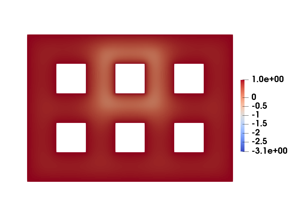 Figure 1
 Figure 2
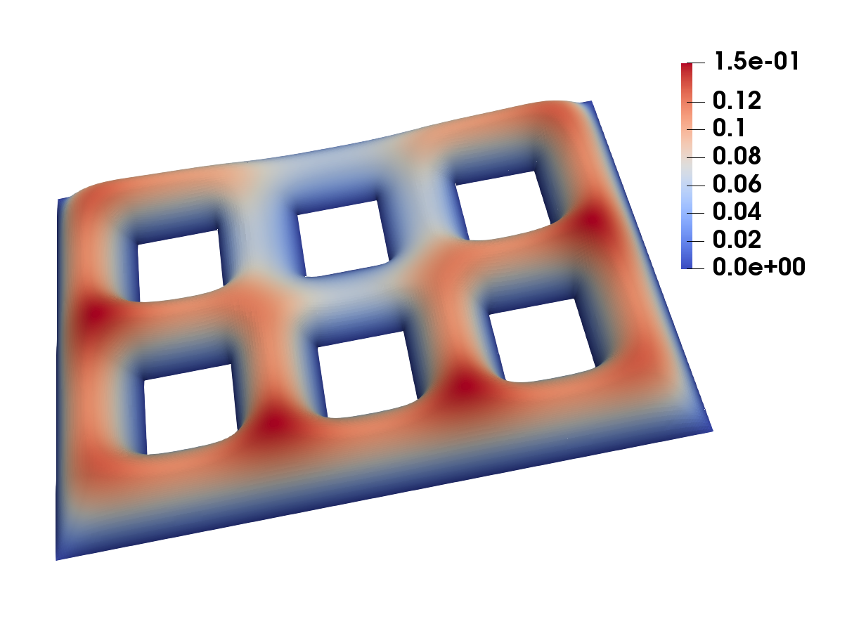 Figure 3
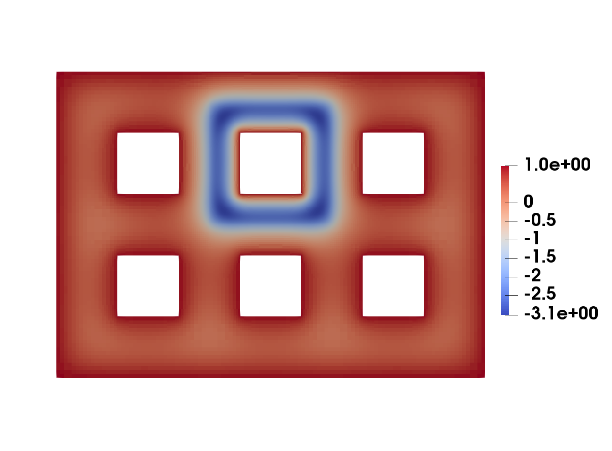 Figure 4
 Figure 5
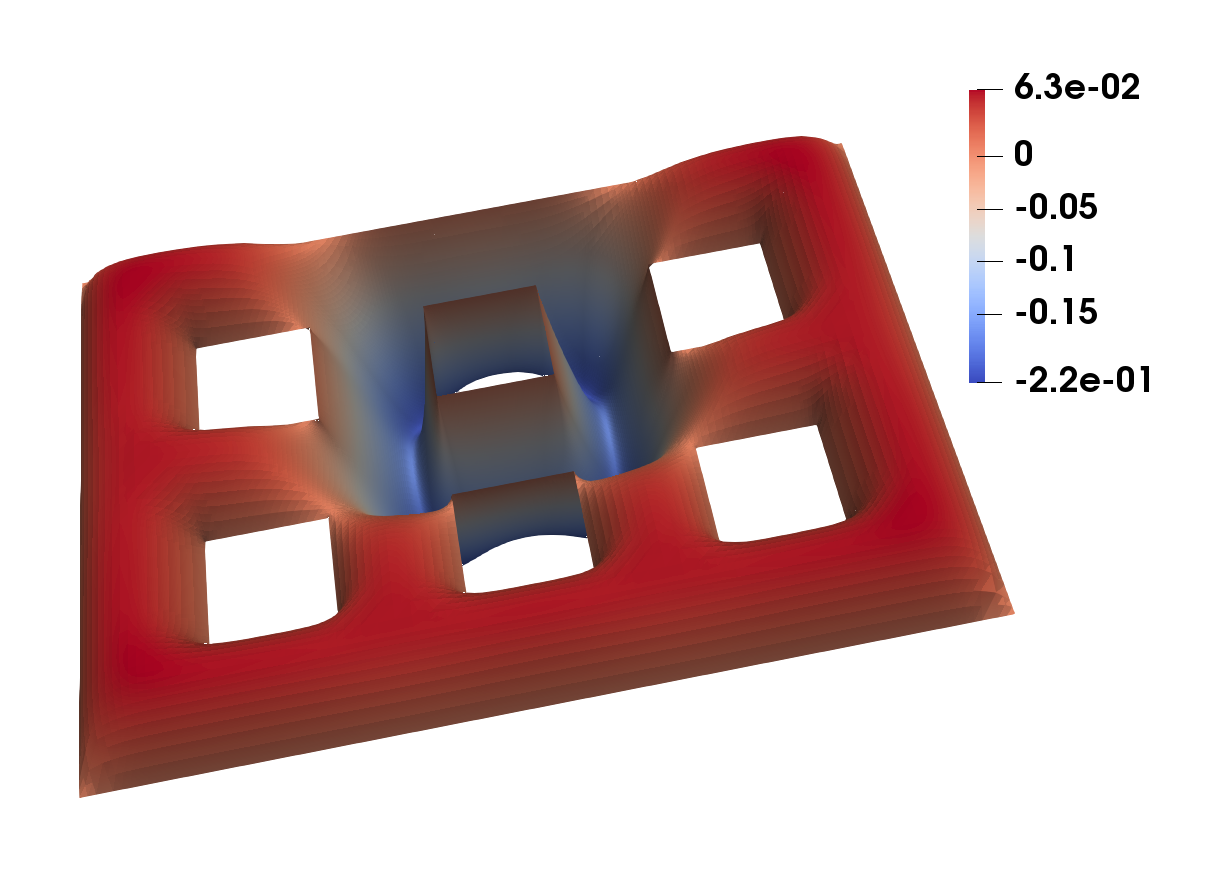 Figure 6
 Figure 7
 Figure 8
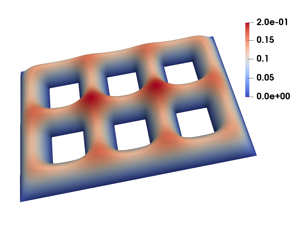 Figure 9
 Figure 10
 Figure 11
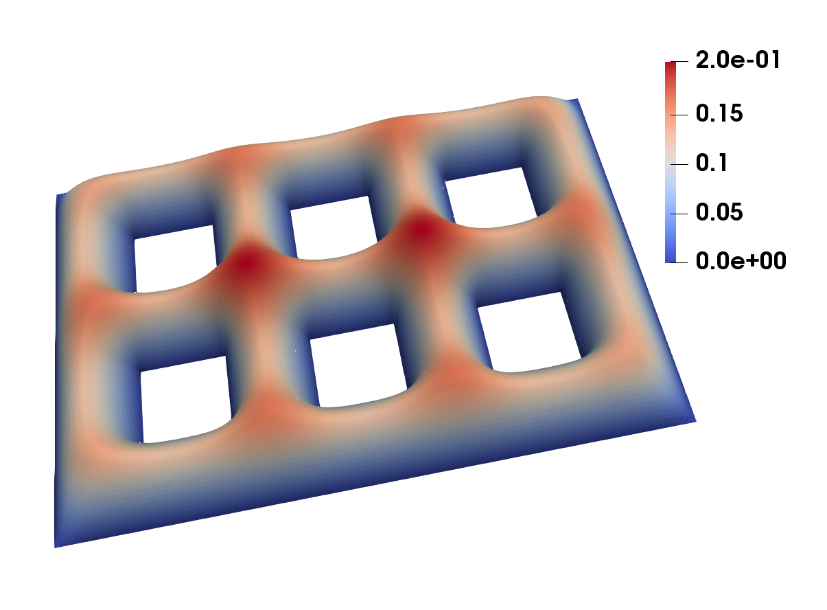 Figure 12
 Figure 13
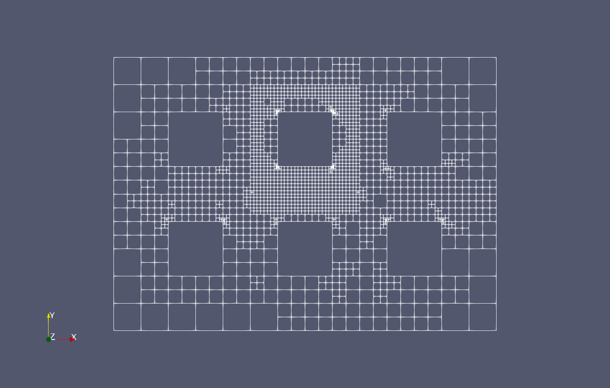 Figure 14
 Figure 15
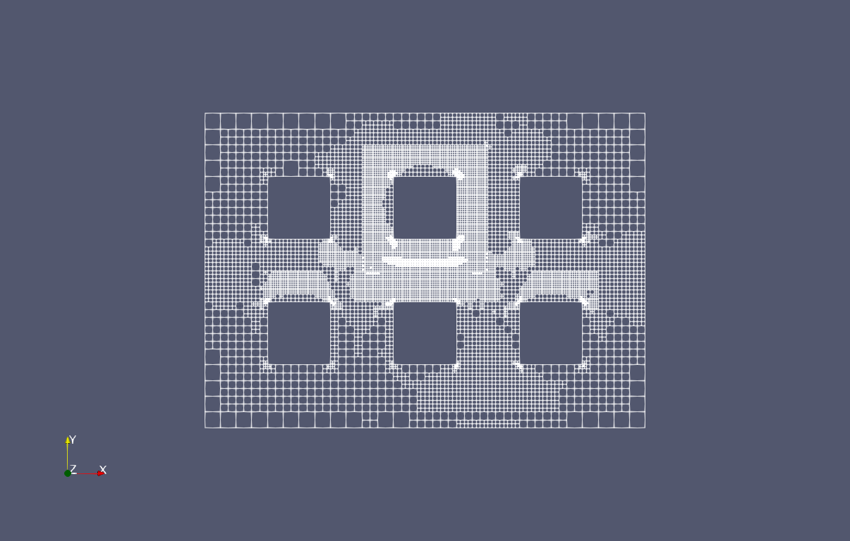 Figure 16
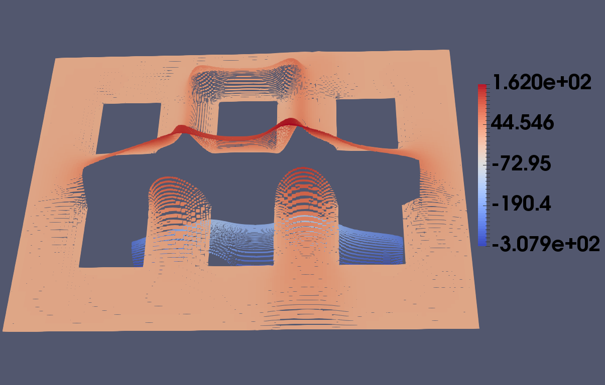 Figure 17
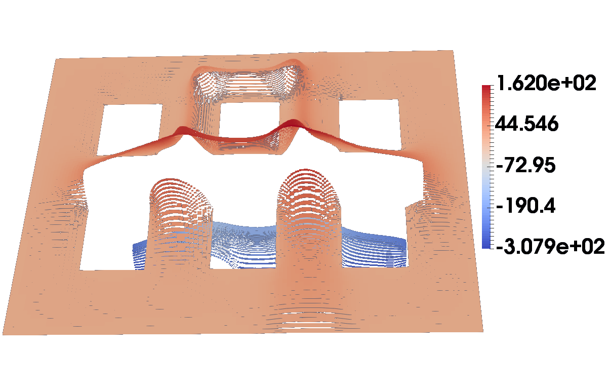 Figure 18
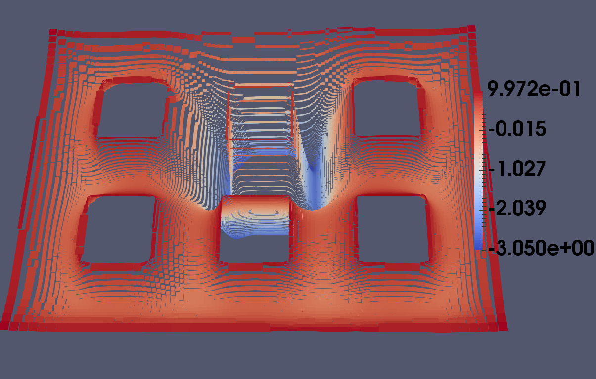 Figure 19
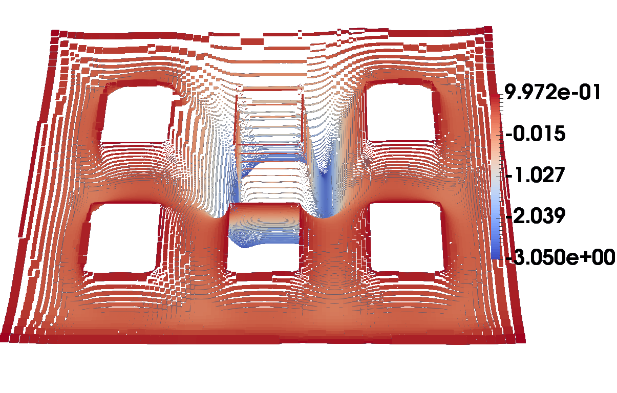 Figure 20
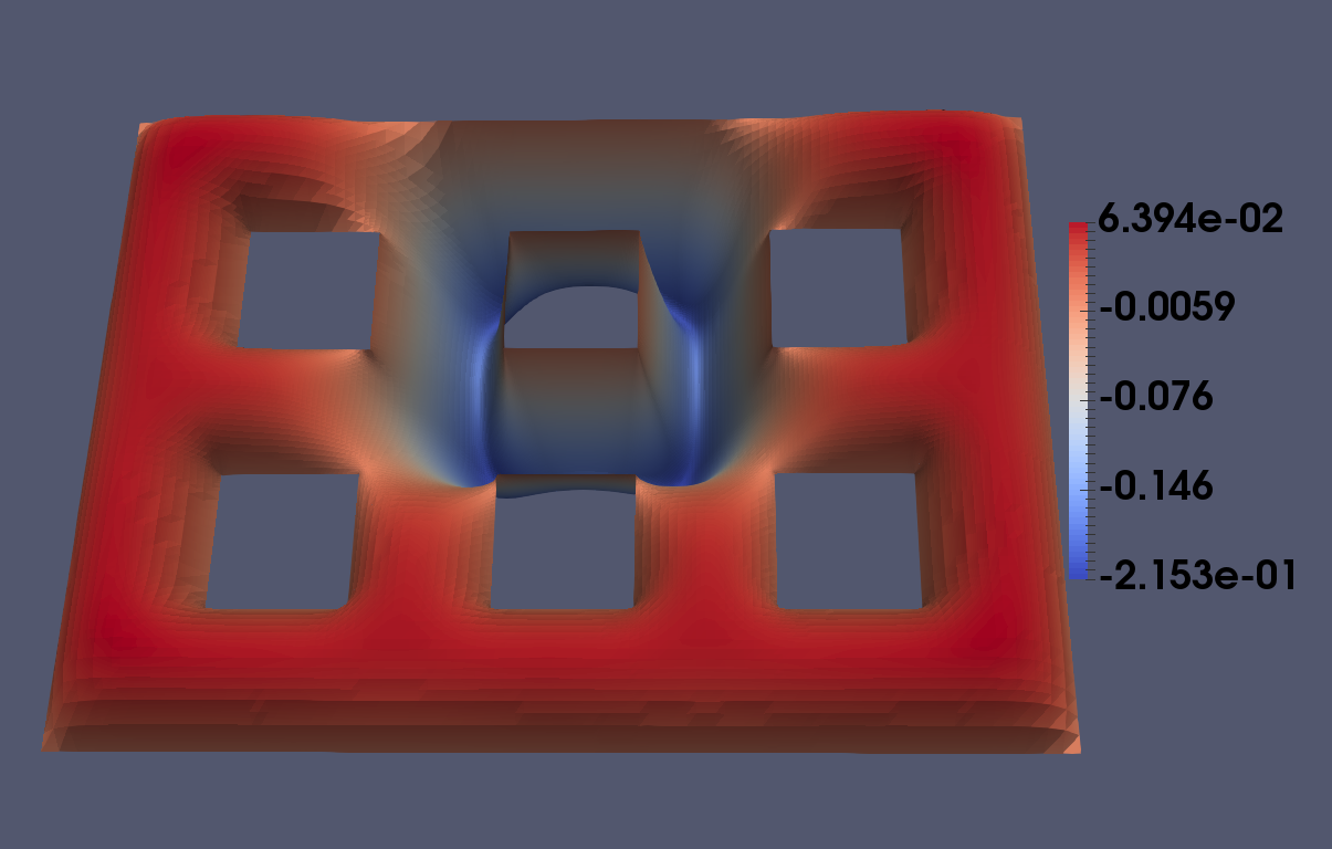 Figure 21
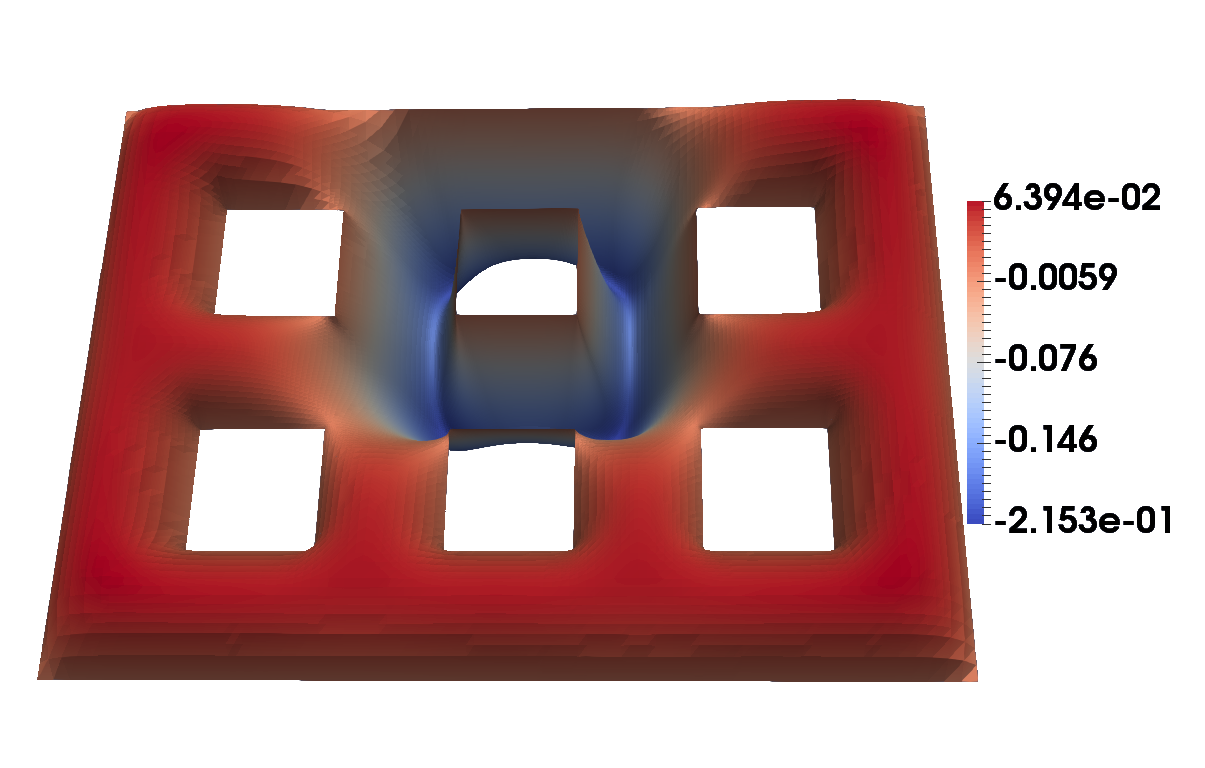 Figure 22
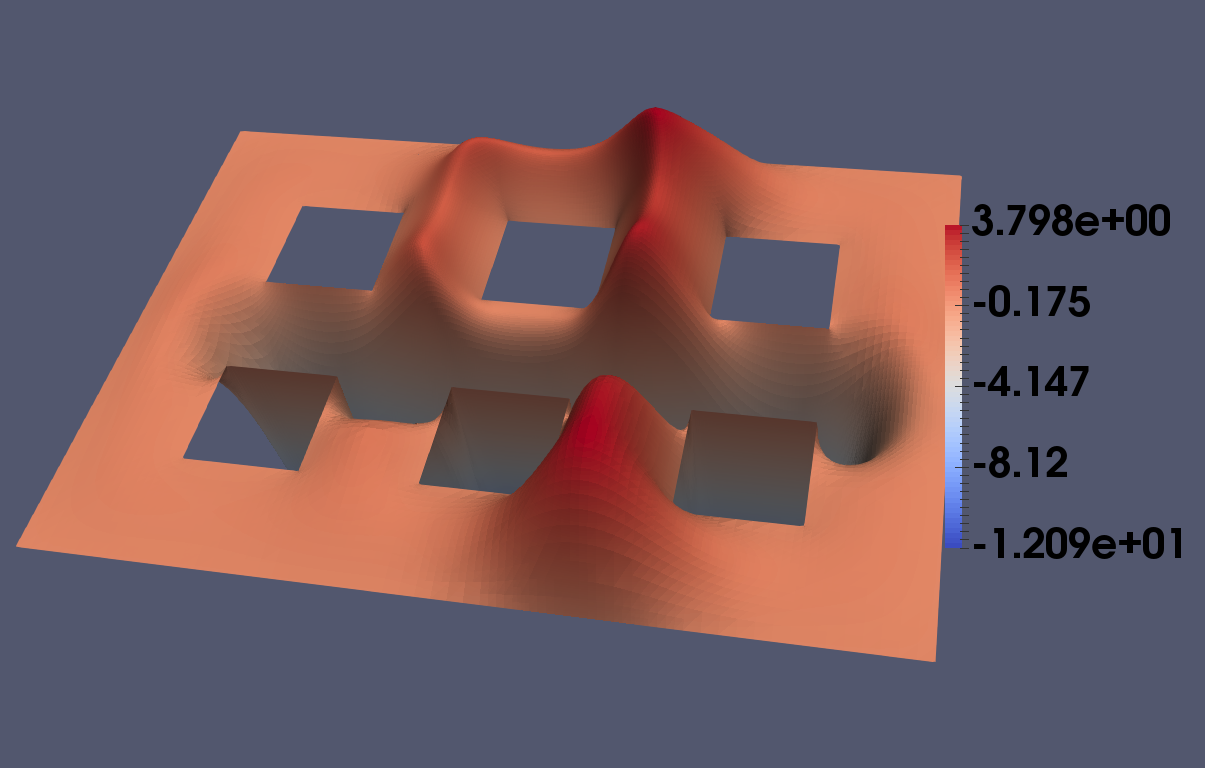 Figure 23
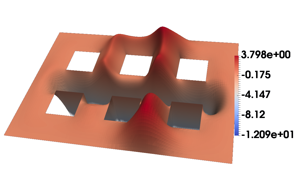 Figure 24
 Figure 25
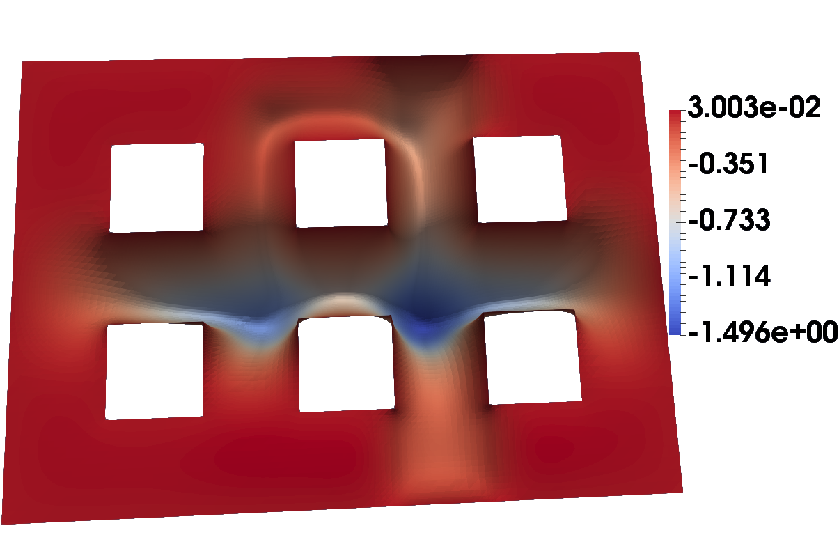 Figure 26
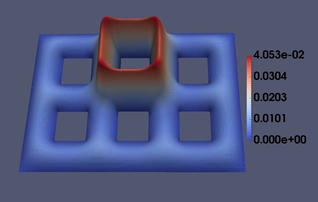 Figure 27
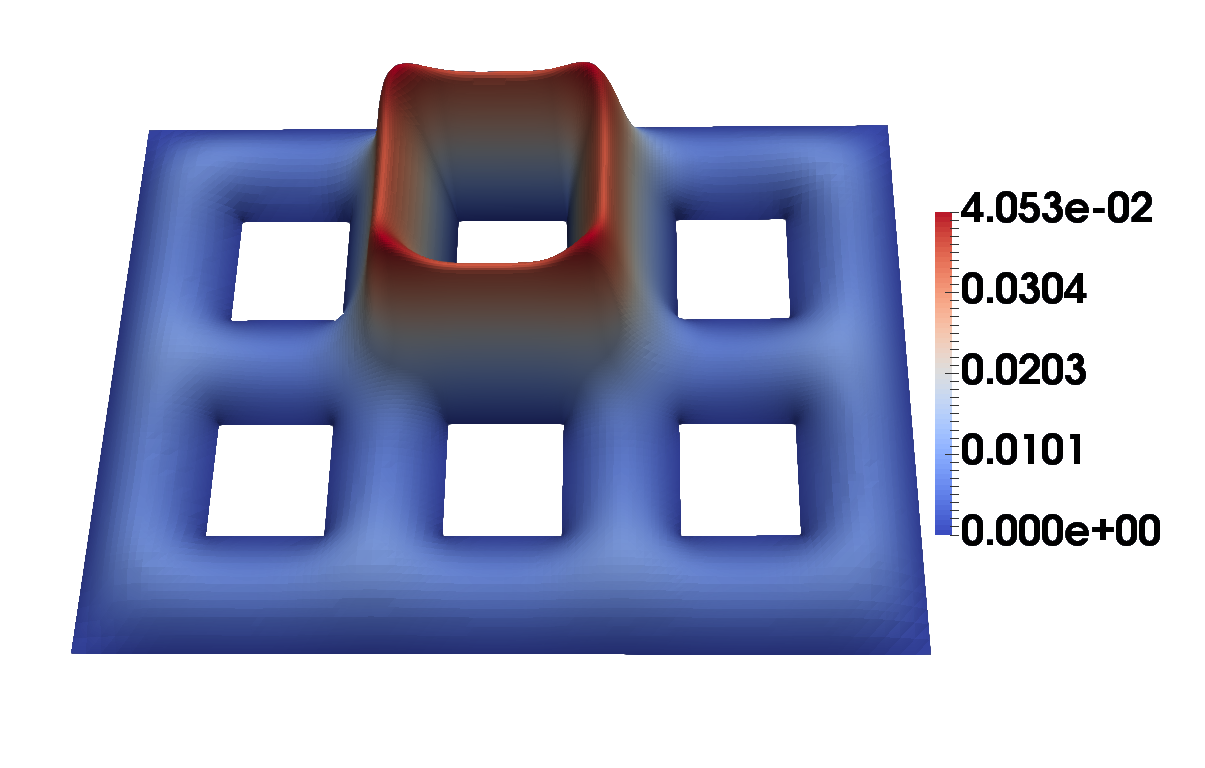 Figure 28
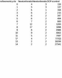 Figure 29
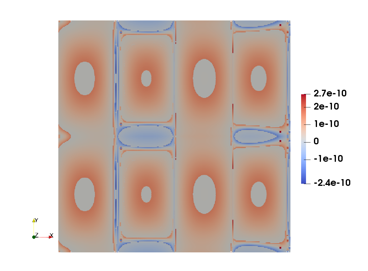 Figure 30
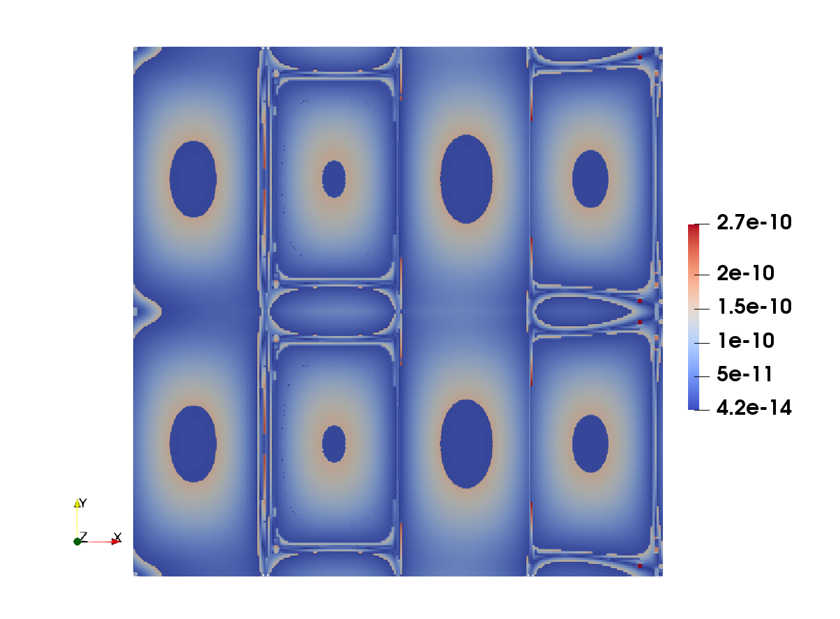 Figure 31
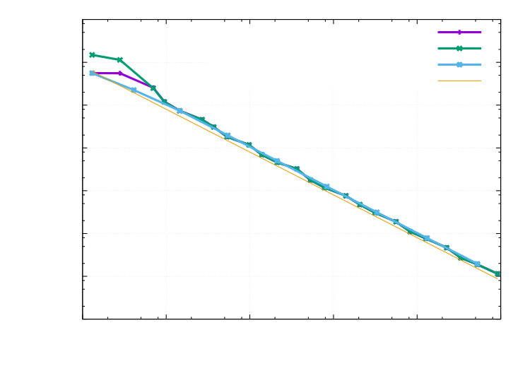 Figure 32
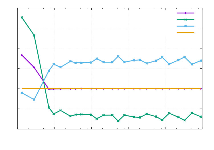 Figure 33
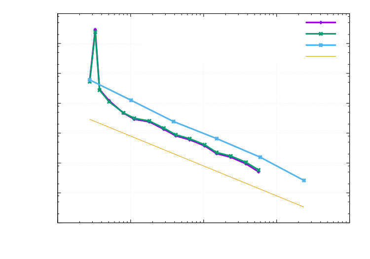 Figure 34
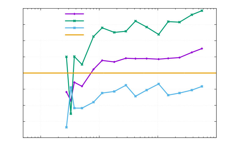 Figure 35
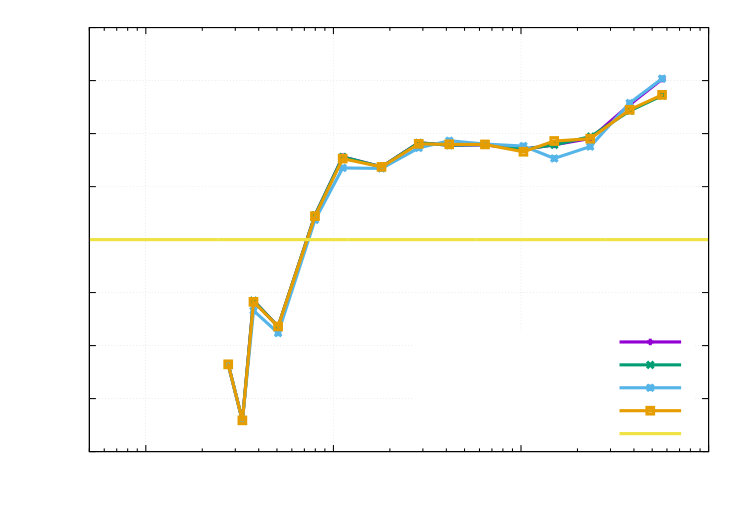 Figure 36
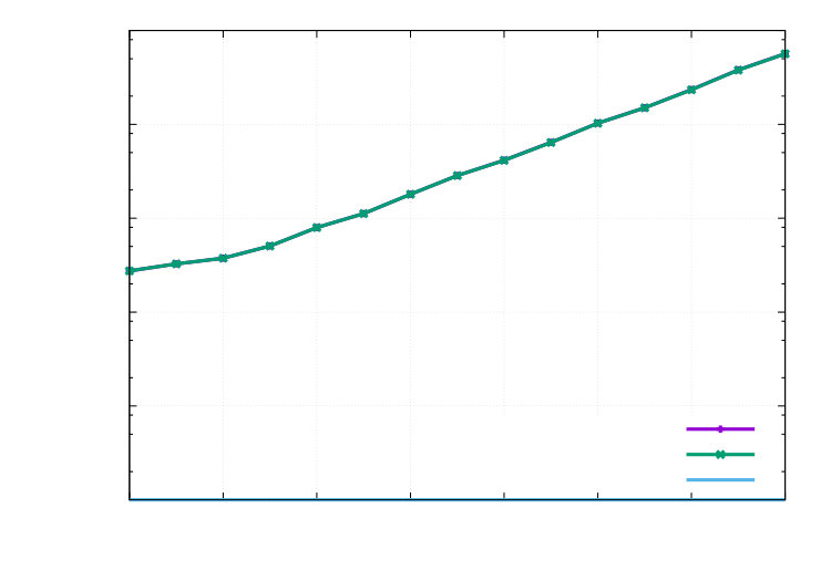 Figure 37
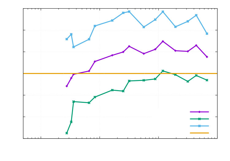 Figure 38
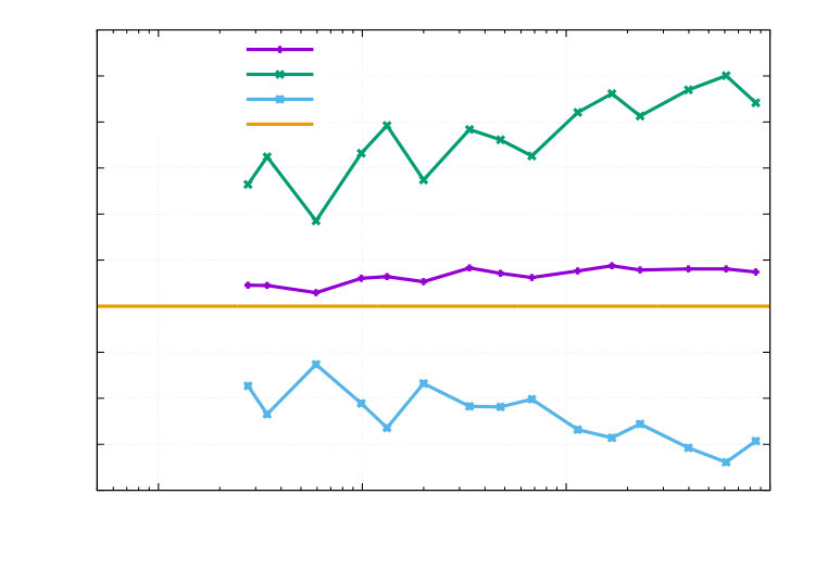 Figure 39
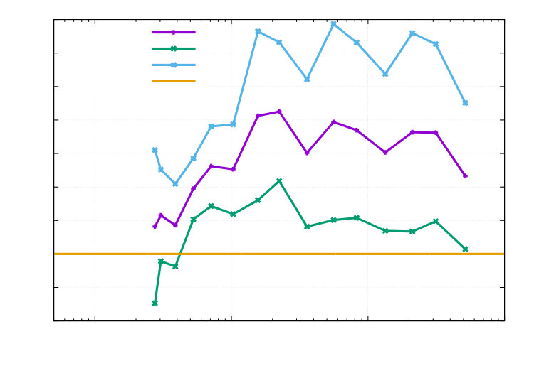 Figure 40
| 0.01 | 0.1 | 1 | 10 | |||||
| DOFs | DOFs | DOFs | DOFs | |||||
| 0 | 0.88 | 275 | 0.69 | 275 | 0.89 | 275 | 0.90 | 275 |
| 1 | 0.94 | 326 | 0.79 | 506 | 0.91 | 565 | 0.93 | 568 |
| 2 | 0.94 | 381 | 0.68 | 759 | 0.91 | 832 | 0.92 | 845 |
| 3 | 0.99 | 561 | 0.66 | 1 266 | 0.92 | 1 367 | 0.93 | 1 451 |
| 4 | 1.05 | 719 | 0.63 | 2 084 | 0.91 | 2 246 | 0.93 | 2 385 |
| 5 | 1.06 | 1 151 | 0.50 | 3 013 | 0.89 | 3 115 | 0.93 | 3 263 |
| 6 | 1.13 | 1 856 | 0.59 | 5 031 | 0.92 | 5 072 | 0.95 | 5 444 |
| 7 | 1.05 | 2 419 | 0.55 | 8 137 | 0.94 | 8 367 | 0.97 | 8 865 |
| 8 | 1.11 | 3 363 | 0.36 | 12 498 | 0.94 | 11 880 | 0.97 | 12 479 |
| 9 | 1.12 | 5 691 | 0.56 | 20 690 | 0.95 | 17 591 | 0.98 | 19 357 |
| 10 | 1.15 | 7 852 | 0.47 | 33 247 | 0.95 | 31 035 | 0.99 | 32 970 |
| 11 | 1.13 | 10 752 | 0.38 | 50 864 | 0.95 | 45 721 | 0.99 | 47 850 |
| 12 | 1.14 | 17 094 | 0.56 | 84 368 | 0.96 | 72 636 | 0.99 | 78 502 |
| 13 | 1.19 | 25 916 | 0.44 | 135 166 | 0.96 | 126 711 | 0.99 | 133 541 |
| 14 | 1.14 | 35 482 | 0.39 | 207 466 | 0.96 | 184 754 | 1.00 | 192 946 |
| DOFs | DOFs | DOFs | DOFs | |||||
| 0.2316036 | 1 326 503 | 0.07069658 | 2 127 499 | 0.1502366 | 1 996 755 | 0.1635741 | 2 107 007 | |
| Error in | Error in | |||
|---|---|---|---|---|
Peer Reviews
No public reviews on file for this paper yet. If you reviewed it on a platform where reviews are public (OpenReview, ICLR, NeurIPS, ICML), you can paste yours below so the community can read it here.
Videos
No videos yet. Explain this paper in a talk, walkthrough, or lecture? Add one.
Multigoal-oriented optimal control problems
with nonlinear PDE constraints
B. Endtmayer
Doctoral Program on Computational Mathematics, Johannes Kepler University, Altenbergerstr. 69, A-4040 Linz, Austria
Johann Radon Institute for Computational and Applied Mathematics, Austrian Academy of Sciences, Altenbergerstr. 69, A-4040 Linz, Austria
U. Langer
Johann Radon Institute for Computational and Applied Mathematics, Austrian Academy of Sciences, Altenbergerstr. 69, A-4040 Linz, Austria
I. Neitzel
Institut für Numerische Simulation, Endenicher Allee 19b, 53115 Bonn, Germany
T. Wick
Institut für Angewandte Mathematik, Leibniz Universität Hannover, Welfengarten 1, 30167 Hannover, Germany
Cluster of Excellence PhoenixD (Photonics, Optics, and Engineering - Innovation Across Disciplines), Leibniz Universität Hannover, Germany
W. Wollner
Technische Universität Darmstadt, Fachbereich Mathematik, Dolivostr. 15, 64293 Darmstadt, Germany
Abstract
In this work, we consider an optimal control problem subject to a nonlinear PDE constraint and apply it to the regularized -Laplace equation. To this end, a reduced unconstrained optimization problem in terms of the control variable is formulated. Based on the reduced approach, we then derive an a posteriori error representation and mesh adaptivity for multiple quantities of interest. All quantities are combined to one, and then the dual-weighted residual (DWR) method is applied to this combined functional. Furthermore, the estimator allows for balancing the discretization error and the nonlinear iteration error. These developments allow us to formulate an adaptive solution strategy, which is finally substantiated via several numerical examples.
1 Introduction
Optimal control problems with nonlinear PDE constraints have been studied for a long time in many works. In particular, employing the (regularized) -Laplacian (see e.g., [29, 22, 34, 46]) as a nonlinear constraint of an optimal control problem was considered for instance in [17].
In many applications, however, not the entire solution is of interest, but only parts or certain quantities of interest, so-called goal functionals. In the past, often a single goal functional was analyzed. However, it may be of interest to control multiple goal functionals simultaneously [33, 32, 48, 28, 35, 42]. In this paper, these three topics are combined: optimal control, the regularized -Laplacian as a numerical example of a quasi-linear PDE constraint, and multiple goal-oriented a posteriori error estimation.
In the following, we briefly refer to studies that treat parts of the three topics. Optimal control problems (specifically, a priori estimates and optimality conditions) with quasi-linear (as the -Laplacian can be classified) elliptic PDE constraints were considered in [16, 18, 15]. More recently, the extension to optimal control with parabolic PDEs was discussed in [9] and [14].
Optimal control problems with (single) goal functionals were investigated in [6, 40, 5, 50, 52, 43]. The -Laplacian and a posteriori error estimates were considered in [36, 12, 20, 13], and, more specifically, for goal functional evaluations, we refer to [34, 44, 25]. To estimate goal functionals, we adopt the dual-weighted residual (DWR) method [7, 8] in which an adjoint problem is solved to obtain (local) sensitivity measures that are used for mesh refinement. As is well-known, using a gradient-based approach for the numerical solution of optimal control problems, the same adjoint problem as for the DWR error estimator can be employed. For this reason, it is natural to combine gradient-based optimization with adjoint-based error estimation.
We are specifically interested in an extended DWR version in which the discretization and (linear/nonlinear) iteration error are balanced [39, 44, 37]. As localization technique we employ integration by parts as done in [8] or, for residual based error estimates, in [49]. The extension of [44] to multiple goal functionals was recently undertaken in [25].
Three major aims constitute the main contents of this paper: first, the design of a framework for goal-oriented error estimation for optimal control subject to a nonlinear PDE and balancing the discretization and nonlinear iteration error (Section 3). From the optimization point of view, we carefully revisit the important elements for the DWR estimator for optimization problems. The main result in this respect is the a posteriori error representation for the reduced optimal control system for an abstract problem formulation. The second aim is the extension to the simultaneous control of multiple goal functionals (Section 4). As a third goal, based on our theoretical developments, we carefully design an adaptive solution algorithm (Section 5). The performance of our algorithms are investigated in terms of the usual quality measures of convergence behavior and effectivity indices in Section 6. The latter one measures the quality of our proposed error estimator in comparison to (known) true errors, which are computed on sufficiently refined meshes.
We summarize the outline of this work as follows: In Section 2, the problem setting is introduced. Next, in Section 3, the dual-weighted residual method for the reduced optimization problem is formulated. The multi-goal approach is then introduced in Section 4. Our algorithmic developments to solve the multiple goal-functional optimal control problem are derived in Section 5. In Section 6, we present several numerical examples that demonstrate the performance of our approach. Therein, we study different Tikhonov regularization parameters, we perform mesh refinement studies, and consider different goal functionals. In Section 7, we summarize the key outcomes of this work.
2 The Optimal Control Problem
In this section, we define an abstract problem formulation and collect some properties that we will rely on when deriving the a posteriori error estimates.
2.1 The Abstract Problem Formulation
Let and be Banach spaces. We would like to find a control and an associated state such that the pair is a local minimizer of some given cost functional , where and have to fulfill the so called state equation with nonlinear differential operator acting between Sobolev spaces. More precisely, the arising PDE-constrained optimization problem reads as follows:
[TABLE]
for some operator , where denotes the dual space of some Banach space . For the theoretical findings in this paper, we assume that, for each , the PDE is uniquely solvable. More precisely, we assume the following:
Assumption 1**.**
Let there exist a unique mapping which is implicitly defined by
[TABLE]
Moreover, we assume that is twice continuously Fréchet differentiable.
Without further mention, we also assume the existence of a at least one global minimizer for Problem (1). For instance, we refer to [47] for general theorems on existence of solutions for problems with linear and semilinear state equations. Moreover, let and be smooth enough for all operations occurring in the next Section.
With the help of the so called control-to-state mapping , we reformulate (1) as an unconstrained optimization problem
[TABLE]
where . Here, we will also assume sufficient smoothness in order to derive all further estimates.
2.2 First Order Necessary Optimality Conditions
It is clear, that under our implicit smoothness assumptions, the first order necessary optimality conditions for a locally optimal control for Problem (2.1) are given by
[TABLE]
For completeness and further use, we rewrite these conditions for the non-reduced formulation with the help of the well-known Lagrange approach. We define the Lagrangian for this problem as follows
[TABLE]
To shorten notation, we consider the abbreviation for the partial derivatives of some operator . The first order necessary optimality conditions for (1) are then given by
[TABLE]
Moreover, denotes the optimal state associated with , and the associated adjoint state. In order for the Newton algorithm to work, and for the error estimator we need the following assumption.
Assumption 2**.**
We assume that is invertible.
2.3 An Example: the Regularized -Laplacian and Tracking-type Cost Functional
Let us finish this section by defining for a concrete example (i.e., a PDE) that motivates our numerical studies. To this end, a (regularized) -Laplace equation for is considered, even though, it does not necessarily fit into the theory setting. For details, we refer to [22, 34, 46] and the references therein regarding the (regularization of) the -Laplace equation. We consider the following setting: Let be open and bounded with boundary, and let . Then we define
[TABLE]
by the identity
[TABLE]
for , where is the usual notation for duality pairings. Note that in this example, we have .
Let be the state, and , e.g., , be the control variable. Then our optimal control problem is given by
[TABLE]
with the tracking-type cost functional
[TABLE]
with and given , and .
3 The Dual Weighted Residual Method for the Reduced System
We now formulate the DWR method for the reduced optimal control system and develop a posteriori error estimators. The presentation is kept as general as possible so that the extension to multiple goal functionals outlined in Section 4 can easily be incorporated. Firstly, we briefly outline the important elements of the discretization.
3.1 Discretization
The method of choice, which will be used in the numerical examples, is the finite element method [19, 11, 31]. However, the algorithms presented in this work can also be adapted to other discretization techniques where adaptivity can be accomplished, like isogeometric analysis, the virtual element method, or finite cell methods. For the spaces , we use continuous tensor product finite elements ;see, for instance, [19]. For we use discontinuous tensor product finite elements . Let be a subdivision (triangulation) of the domain into quadrilateral elements such that and for all where . Furthermore, let be a multilinear mapping from the reference element to the element . We define the space as
[TABLE]
with . The use of these finite dimensional spaces leads to a conforming discretization for Example 2.3. We point out that the conforming discretization is needed in order to keep Theorem 3.5 valid. The discretized abstract model problem reads as follows: Find and such that they are a local solution pair of
[TABLE]
Assumption 3**.**
There exists a unique discrete mapping , which is implicitly defined by
[TABLE]
As for its continuous counterpart, we assume that it is twice continuously Fréchet differentiable.
Using the discrete mapping , we can reformulate Problem (7) as the unconstrained optimization problem: Find such that it solves
[TABLE]
Similar to Section 2.2, we also provide the discrete version of the first order necessary optimality conditions. If is a local solution, then these conditions are given by
[TABLE]
We will also use the non-reduced formulation with the help of the Lagrange-approach, with
[TABLE]
The discrete first order necessary optimality conditions for (7) are then given by
[TABLE]
where and .
3.2 Error Representation for the Reduced System
We are now interested in an error estimator for a quantity of interest . Let be an optimal control of Problem (2.1) with associated optimal state . While we are interested in , we can only compute an approximation of this value. Note that we assume, for most of what follows, that is exactly solved by means of the solution operator for the discrete state equation, cf. Section 3.1. To estimate this error, we apply the previously mentioned DWR method (e.g., [8]) to the first order optimality conditions of our reduced system.
Defining as well as , the error between and can be split into
[TABLE]
Therefore, still corresponds to our "true" quantity of interest, but computed with the discrete solutions and . We start by estimating the first part of the error, which actually has a practical relevance: if some approximate control is computed and applied in a practical situation, then the corresponding physical system will produce a "true" state instead of an approximation .
As a first result, we formulate a theoretical error estimator, where we need the adjoint problem to the first order optimality conditions, which is given by: Find such that
[TABLE]
Assumption 4**.**
We assume that (11) has a unique solution.
Theorem 3.1** (Error Representation for Reduced System).**
Let us assume that and . If solves (2.1) and solves (11) for , then, for arbitrary fixed and , we find:
[TABLE]
where
[TABLE]
and the remainder term satisfies
[TABLE]
with and .
Proof.
The proof follows the same idea as in [44, 25] but is stated for completeness of presentation. Define and as above and let , , be defined as , , as well as . Furthermore, let be defined . By the fundamental theorem of calculus as well as the trapezoidal rule, we observe that
[TABLE]
By carefully inspecting , it follows that it coincides with . Additionally, we can deduce that
[TABLE]
due to (3) and (11). Combining (13) and (14) results in the following identity
[TABLE]
Therefore, using again (3) as well as (12), we get
[TABLE]
where we have applied (15). This proves the theorem after verifying that . ∎
Remark 3.2**.**
One objective of this representation, in addition to the fact that for instance is not readily available exactly, is to obtain indicators for local adaptivity. By inspecting the primal part of the error estimator , we observe that
[TABLE]
Since it is not clear how to localize , we do not follow this path to compute the error indicators, but prove a localizable error estimator in a similar fashion in Theorem 3.5, which makes use of (5) as well.
For another idea, we consider the adjoint problem to the first order optimality conditions for the Lagrangian defined in (4): Find such that
[TABLE]
where the argument in the partial derivatives is always given by .
Assumption 5**.**
We assume that (16) has a unique solution.
In order to obtain the variables and with the help of the solution of the reduced adjoint problem (11), the following lemma is useful.
Lemma 3.3**.**
If with associated state is a local solution of (2.1), and solves (11), then , , and given by (21) solve (16).
Proof.
Let be arbitrary. Using the definition of the reduced functionals, we obtain
[TABLE]
and
[TABLE]
Furthermore, with the definition of the solution operator, we obtain from (2) that
[TABLE]
and
[TABLE]
By subtracting (19) from (17), it follows that
[TABLE]
Further, from (18) we get
[TABLE]
Thus and satisfy the third line in (16).
To proceed, we note that , and solves (5), thus we have that . This leads to
[TABLE]
Now, we define by the first line of (16), we get
[TABLE]
With this, we can rewrite (20) as
[TABLE]
Now, we can use the definition of , , the formula for and the representation of to get
[TABLE]
and the second line in (16) follows. ∎
Lemma 3.3 allows to obtain by solving the reduced adjoint equation (11). Then, can be computed by solving the tangent equation
[TABLE]
which is the last row of (16). Using this solution, we can deduce from the first row of (16).
An analogue to (16) on the discrete level is given by: Find such that
[TABLE]
where the arguments in the partial derivatives are given by .
Remark 3.4**.**
If (22) is considered at the linearization point , then Lemma 3.3 holds also true for the discrete problem, i.e. if solves
[TABLE]
then . This can be shown by the same proof replacing by .
Similar as explained above, the variables and can be deduced from the knowledge of and the discrete version of Lemma 3.3.
Theorem 3.5** (Localizable Error Representation for Reduced System).**
Let us assume that and . Let be a local solution of (2.1), with the corresponding KKT-triplet given by (5), and let the triple solve (16). Moreover, let be an arbitrary fixed discrete control, and let be the solution to (10) and the first and last row of (22) at the linearization point with and . Then we have the error representation
[TABLE]
where
[TABLE]
and the remainder term
[TABLE]
with , .
Proof.
The proof follows a similar structure as the proof of Theorem 3.1. Let , . For we define . It holds that
[TABLE]
where . By carefully inspecting it follows that
[TABLE]
since and . Thus, (25) gives
[TABLE]
For the part of (25), we can deduce that
[TABLE]
since solves (16) and solves (5). Finally, relation (25) reduces to the following identity
[TABLE]
Therefore, we get
[TABLE]
Furthermore, we can deduce that . Gathering the results from above, we obtain, noting that
[TABLE]
Straightforward calculations show
[TABLE]
and
[TABLE]
∎
Let us end this section with some further observations.
Remark 3.6**.**
Note that if , then in fact solve (10), cf. Remark 3.4, and consequently .
Remark 3.7**.**
From numerical experiments for the regularized -Laplacian computed in [27], we can deduce that can be neglected on sufficiently refined meshes.
An identity also observed in [51], is the following:
Proposition 3.1**.**
If and is injective, then we have .
Proof.
Since is the cost functional and is a local minimizer of our optimization problem the first order necessary condition is given by . Therefore the adjoint equation reads as
[TABLE]
If is injective, then . From the tangent equation
[TABLE]
we can deduce that . Finally the optimality system reduces to
[TABLE]
From this follows that , which completes the proof. ∎
3.3 The Parts of the Error Estimator
We now briefly discuss the two main parts of the error estimator:
[TABLE]
where the first part refers to the iteration error, and the second term denotes the discretization error to be defined in the following. We recall that is designed to estimate given in (24).
The iteration error estimator
The iteration error estimator
[TABLE]
can be used as stopping rule for the nonlinear solver like for Newton’s method as in [44, 25, 25] and Algorithm 1 presented in Section 5.
The discretization error estimator
Of course the exact solution of the optimal control problem in formula (24) are not known. They can either be replaced by a (patch-wise) higher order polynomial interpolation or by approximations on enriched spaces [8, 4].
The discretization error estimator using the solutions and on enriched spaces reads as
[TABLE]
The replacement is justified if a strengthened saturation assumption is fulfilled as shown in [27] for both the nonlinear state equation and the goal functionals.
We briefly recall that the localization can be performed in three ways: classical integration by parts yielding the strong problem formulation [8], a filtering approach employing the weak problem formulation [10], or a partition-of-unity using again the weak form of the problem [45]. All three techniques are analyzed (theoretically and computationally) with respect to their effectivity in [45]. In the theoretical analysis, a discrete version of Lemma 3.3 is necessary to justify that is indeed a solution in the enriched spaces.
4 Extension to Multiple Goal Functionals
In Section 3, we discussed how the DWR method works for one functional. However, for some problems, several functional evaluations would be of interest. Let us consider goal functionals for some . One possibility would be to compute the error estimators separately as described in Section 3. However, we would have to solve the adjoint problem times, leading to high computational cost. There are several ways to tackle this problem as for example discussed in [33, 32, 42, 1] and more recently in [35, 28, 25, 26, 27].
Adopting the techniques presented in [25], we try to combine the functionals to one, and apply the DWR method for one functional to it. In the following section, we consider , as the solution of (1), and , as some approximations. To construct the combination, we introduce a so called error weighting function:
Definition 4.1** (Error weighting function [25]).**
Let . We say that is an error-weighting function if is strictly monotonically increasing in each component and for all .
As in [25], let mapping from . Furthermore, we define as the component-wise absolute value. This allows us to construct the error function as follows:
[TABLE]
Remark 4.2**.**
The error functional is constructed in a way, that avoids error cancellation between two or more functionals. For a more detailed discussion, we refer the reader to [25, 27].
Remark 4.3**.**
The quantity (30) is not computable, since it depends on , which is not known. However, we can use a higher order polynomial approximation to approximate this quantity, as done in [33, 25, 27], where consequences of the replacement are discussed in [27].
The resulting error weighting functional is given by
[TABLE]
where , denote the solutions on enriched finite element spaces.
Remark 4.4**.**
We notice that, for the choice , we obtain the same combined functional as in [28] up to sign. The same holds for [33, 32] in the case of linear problems. This choice is used in our numerical examples.
Remark 4.5**.**
Finally, the method explained in Section 3 is applied to instead of to achieve a control of the errors in all functionals at once, as algorithmically illustrated in Section 5.
5 Algorithmic Details
In this section, we briefly recapitulate the algorithmic techniques to solve the optimal control problem with multiple goal functionals that we have outlined in the previous sections. The algorithms for the forward problem including multiple goal functionals evaluations were derived in [25]. Therein, the goal functionals were estimated using the DWR method (thus an adjoint approach). Hence, the extension to optimal control using a gradient-based approach is straightforward. The implementation of the following algorithms is done in the open-source library DOpElib [23, 30]. For a general overview of optimization algorithms, we refer to [41, 38]. First, we present the reduced Newton method described in Algorithm 1.
Remark 5.1**.**
The parameter is chosen as in the numerical experiments.
Remark 5.2**.**
In [30], we specifically used DOpE::ReducedNewtonAlgorithm::ReducedNewtonLineSearch to obtain the line search parameter .
Remark 5.3**.**
*The arising linear problems and
were solved by using the algorithm
DOpE::ReducedNewtonAlgorithm::SolveReducedLinearSystem implemented in [30].*
With the help of Algorithm 1, we can now state the final Algorithm 2 used in this paper.
Remark 5.4**.**
In Algorithm 2 in Step 8, we use Dörfler marking with as marking strategy [24].
Remark 5.5**.**
The reduced discrete cost functional on the space is constructed by means of the corresponding discrete solution operator on the enriched space.
Remark 5.6**.**
To solve the linear systems arising form the forward state equation, we use the sparse direct solver UMFPACK [21].
6 Numerical examples
In the current section, we provide some numerical examples demonstrating the performance of the theoretical arguments and algorithms developed previously. The implementation is done in DOpElib [23, 30] using the finite elements from deal.II [3, 2]. However, large parts of the programming are new . For this reason, we first present a linear example with a single goal functional, which has been already studied in the literature. In the second example, we then consider the -Laplacian and again the case of a single goal functional. In Example 3, we study several nonlinear goal functionals that are simultaneously controlled. The quality of our results will be measured by effectivity index which is given by
[TABLE]
whereas the primal and adjoint effectivity indices are defined by
[TABLE]
and
[TABLE]
Notice that we do not apply the absolute value to the contributions. Hence, we also estimate the sign of the error.
6.1 Example 1: linear Laplacian, single goal functional
In this first numerical test, we consider a standard linear example, which is implemented, for instance, in DOpElib[23, 30][OPT/StatPDE/Example1, Section 6.1.1]. The main purpose is to validate our novel programming code against known findings. The domain is . The right-hand side forces of the PDE are f(x,y):=\big{(}20\pi^{2}\text{sin}(4\pi x)-\alpha^{-1}\text{sin}(\pi x)\big{)}\text{sin}(2\pi y). The given control is , and the desired state is u^{d}:=\big{(}5\pi^{2}\text{sin}(\pi x)+\text{sin}(4\pi x)\big{)}\text{sin}(2\pi y). The regularization is chosen as .
The problem statement is as follows: Find such that it is a minimizer of
[TABLE]
with the constraints
[TABLE]
The exact minimizer of the problem is known, and given by and . First of all, we use , so the cost functional as quantity of interest. Here, the exact value is given by J(\overline{u},\overline{q})=\frac{1}{8}\big{(}25\pi^{4}+\alpha^{-1}\big{)}.
In the Figures 1 and 2, the effectivity index and the error are both shown against the number of degrees of freedom (DOFs). For the single error parts, primal and adjoint estimators, the effectivity indices show significant differences from the asymptotically expected value. Combining both parts, then yields an optimal . Convergence of adaptive and uniform mesh refinement are shown in Figure 2.
1e-050.00010.0010.010.1110100101001000100001000001e+06DOFsError in (adp.)Estimated ErrorError in (uni.)
1e-050.00010.0010.010.1110100101001000100001000001e+06DOFsError in (adp.)Estimated ErrorError in (uni.)
In this second part of the example, we apply the method to a quantity that is different to the cost functional. We are interested in . The exact value is given by . The corresponding numerical findings are displayed in the Figures 3 and 4. We observe excellent effectivity indices in Figure 3. Optimal convergence rates also in comparison with uniform mesh refinement are observed in Figure 4.
-2.5-2-1.5-1-0.500.511.522.5101001000100001000001e+06DOFsI_{eff}$$I_{effp}$$I_{effa}1
1e-050.00010.0010.010.1110101001000100001000001e+06DOFsError in (adp.)Estimated ErrorError in (uni.)
6.2 Example 2: -Laplacian, single goal functional
We now proceed to nonlinear state equations and consider the example PDE provided in Section 2.3. Here, (and the initial mesh) and are given in Figure 5. Furthermore, , , and . In particular, we investigate various regularization parameters . The goal functional is given by .
In Table 1, we obtain, for , effectivity indices in the range of to , which are excellent findings in view of the nonlinear behavior of the state equation and the geometric singularities introduced by the domain. In the case of , we obtain a in the range of to , which might be affected by cancellation effects from adding the different contributions to the error estimator. The exact value of the functionals was approximated by one additional and refinement, and is given in the last line of Table 1 corresponding to , with additional information on the number of DOFs used to compute this values.
In the Figures 6 and 7, the final meshes for different are shown. For , we observe very localized mesh refinement, while, for larger , the mesh is still locally refined, but in a somewhat uniform behavior. The states and controls on these final meshes are displayed in the Figures 8 and 9.
6.3 Example 3: -Laplacian, multiple goal functionals
In this third example, we proceed to multiple goal functionals. The setup is the same as in Example 2, but with a single and multiple goal functionals:
- •
,
- •
,
- •
,
- •
,
- •
.
The geometry alongside with the goal functionals and is illustrated in Figure 10.
0.60.70.80.911.11.21.31.4100100010000100000DOFsI_{eff}$$I_{effp}$$I_{effa}1
0.00010.0010.010.111010010001001000100001000001e+06DOFsError in (adp.)Estimated ErrorError in (uni.)
1e-050.00010.0010.010.11101001000100100010000100000DOFsI_{1}$$I_{2}$$I_{3}$$I_{4}$$I_{5}$$I_{\mathfrak{E}}
1e-050.00010.0010.010.11101001000100100010000100000DOFs\eta_{h}^{(2)}$$\rho_{u}$$\rho_{p}$$\rho_{z}$$\rho_{v}$$\rho_{q}$$\rho_{y}
The reference values are computed on a fine grid ( DOFs for + DOFs for ) , which is obtained by 12 adaptive refinements for followed by two uniform h-refinements and one uniform p-refinement. Our findings are displayed in the Figures 11, 12, 13 and 14. In Figure 11 the calculated effectivity indices are excellent in view of the nonlinearities of the domain, state equation and multiple goal functionals. Curves of the errors and estimators are shown in the Figures 12, 13 and 14. Here, the combined functional (as expected) bounds all single functionals. In Figure 12, we observe that adaptive refinement pays off in delivering the same error as uniform mesh refinement, but with a lower computational cost. The convergence rates are the same, which lies in the fact that the control is chosen in such a way that a sufficiently smooth final solution is obtained. Finally, we compare the adaptive stopping rule used in Algorithm 1 with the standard stopping rule, which is used in the DOpElib [23, 30] algorithm DOpE::ReducedNewtonAlgorithm::Solve with the absolute residual nonlinear_global_tol = 1.e-7 and relative residual nonlinear_tol= 8.e-5. Since the discretization error estimate is not given for in Algorithm 1, we use .
We abbreviate the first algorithm with AN (Adaptive Newton) and the second algorithm with FN (Full Newton). In Table 2, we monitor that the show a pretty similar behavior even for the adaptive stopping rule. Even though we need iterations in case of the adaptive stopping rule compared to iterations for the standard stopping rule, which is illustrated in Table 2 as well. Furthermore, we want to notice that the refined meshes for both algorithms coincide exactly up to . For , it is exactly one element, which is refined additionally in the case of FN. If we compare the corrected effectivity indices
[TABLE]
for the two stopping rules, we observe that they coincide even more after the correction.
In Table 3, the comparison between the estimated iteration error and the real error in the combined functional is shown. The ratio between and the error mimics the choice of in Algorithm 1 for our adaptive stopping rule, whereas there is almost no correlation for the standard stopping rule.
7 Conclusions
In this work, we developed a novel a posteriori multiple goal-oriented error estimation for optimal control problems subject to a nonlinear state equation. The error estimator also serves for balancing the discretization and nonlinear iteration error. The overall optimization problem is solved via a reduced approach in which the state equation is eliminated by a control-to-state solution operator. In Section 3.2, the theoretical results yield an a posteriori estimate for a single goal functional. The extension to multiple goal functionals was made in Section 4. Based on these theoretical aspects, the algorithmic details were worked out in the following section. Three numerical examples were investigated. In the first example, our approach was tested against configurations known in the literature. The Examples 2 and 3 are more advanced by considering the regularized -Laplacian as nonlinear state equation. The main criterion whether the proposed error estimator works sufficiently well is given by the effectivity index. In the numerical examples, values around one were obtained. These are excellent findings in view of the challenging nature of the underlying problem configuration; namely domain (corner) singularities, quasi-linear state equations within an optimal control setting, and finally multiple nonlinear goal functionals. Ongoing work considers the extension to elasticity and more practical applications.
8 Acknowledgments
This work has been supported by the Austrian Science Fund (FWF) under the grant P 29181 ‘Goal-Oriented Error Control for Phase-Field Fracture Coupled to Multiphysics Problems’ and the DFG-SPP 1962 ‘Non-smooth and Complementarity-based Distributed Parameter Systems: Simulation and Hierarchical Optimization’ within the project ‘Optimizing Fracture Propagation Using a Phase-Field Approach’ under grant numbers NE1941/1-1 and WO1936/4-1.
The reference list from the paper itself. Each links out to its DOI / PubMed record.
- 1[1] J. Alvarez-Aramberri, D. Pardo, and H. Barucq. Inversion of magnetotelluric measurements using multigoal oriented hp-adaptivity. Procedia Computer Science , 18:1564–1573, 2013.
- 2[2] W. Bangerth, D. Davydov, T. Heister, L. Heltai, G. Kanschat, M. Kronbichler, M. Maier, B. Turcksin, and D. Wells. The deal.II library, version 8.4. J. Numer. Math. , 24(3):135–141, 2016.
- 3[3] W. Bangerth, R. Hartmann, and G. Kanschat. deal.II – a general purpose object oriented finite element library. ACM Trans. Math. Softw. , 33(4):24/1–24/27, 2007.
- 4[4] W. Bangerth and R. Rannacher. Adaptive Finite Element Methods for Differential Equations . Birkhäuser Verlag, Boston, 2003.
- 5[5] R. Becker, M. Braack, D. Meidner, R. Rannacher, and B. Vexler. Adaptive finite element methods for PDE-constrained optimal control problems. In Reactive flows, diffusion and transport , pages 177–205. Springer, Berlin, 2007.
- 6[6] R. Becker, H. Kapp, and R. Rannacher. Adaptive finite element methods for optimal control of partial differential equations: Basic concept. SIAM J. Control Optim. , 39(1):113–132, 2000.
- 7[7] R. Becker and R. Rannacher. A feed-back approach to error control in finite element methods: Basic analysis and examples. East-West J. Numer. Math. , 4:237–264, 1996.
- 8[8] R. Becker and R. Rannacher. An optimal control approach to a posteriori error estimation in finite element methods. Acta Numer. , 10:1–102, 2001.