Large Transverse Momentum in Semi-Inclusive Deeply Inelastic Scattering Beyond Lowest Order
B. Wang, J. O. Gonzalez-Hernandez, T. C. Rogers, N. Sato

TL;DR
This paper revisits second-order calculations of large transverse momentum in semi-inclusive deep inelastic scattering, confirming previous results and highlighting discrepancies with existing parton distribution and fragmentation functions.
Contribution
It provides a detailed second-order calculation of the transverse momentum dependence, supporting the existence of tension with current parton functions.
Findings
Confirmation of previous $O(\alpha_s^2)$ calculations
Identification of tension with current parton distribution functions
Reinforcement of the need for improved theoretical models
Abstract
Motivated by recently observed tension between calculations of very large transverse momentum dependence in both semi-inclusive deep inelastic scattering and Drell-Yan scattering, we repeat the details of the calculation through transversely differential cross section. The results confirm earlier calculations, and provide further support to the observation that tension exists with current parton distribution and fragmentation functions.
Click any figure to enlarge with its caption.
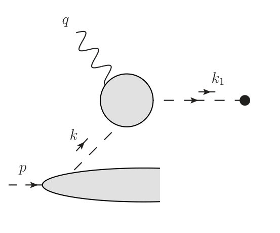 Figure 1
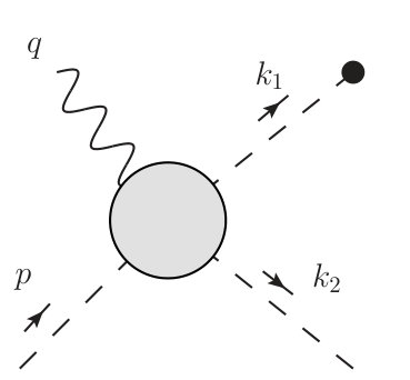 Figure 2
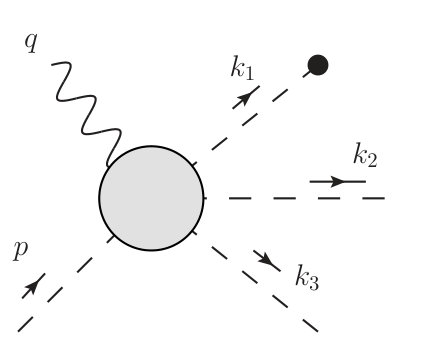 Figure 3
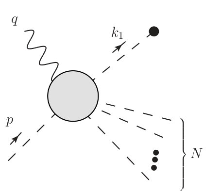 Figure 4
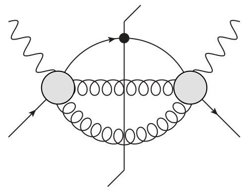 Figure 5
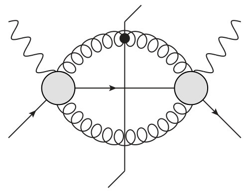 Figure 6
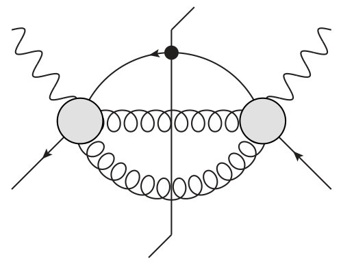 Figure 7
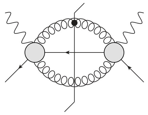 Figure 8
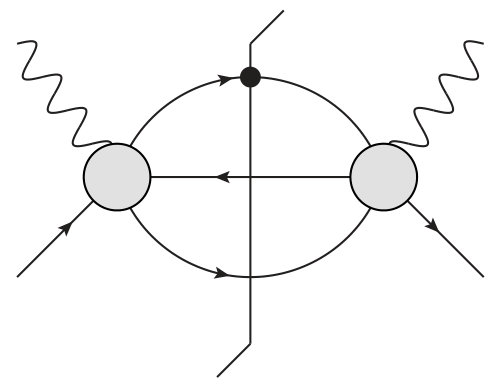 Figure 9
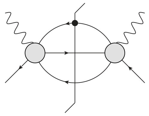 Figure 10
 Figure 11
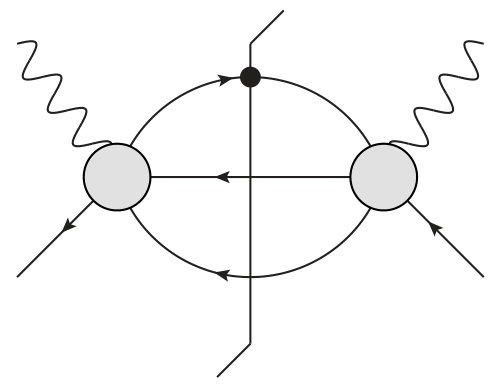 Figure 12
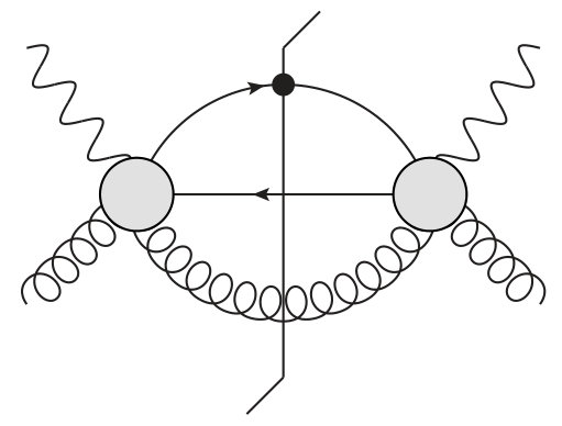 Figure 13
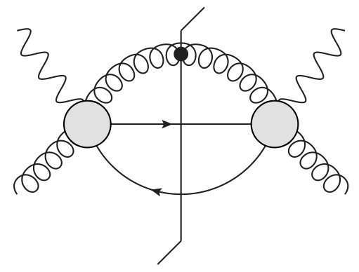 Figure 14
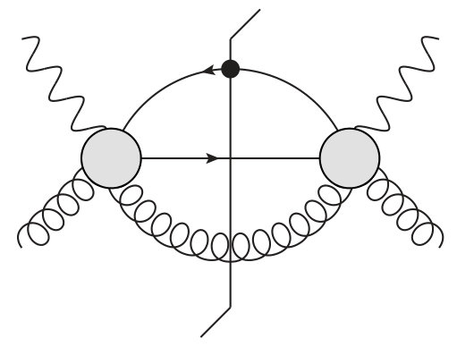 Figure 15
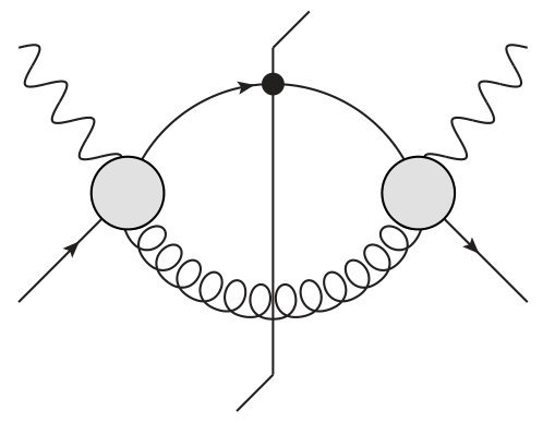 Figure 16
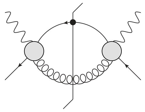 Figure 17
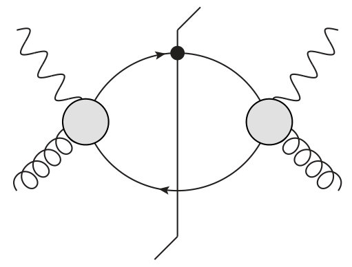 Figure 18
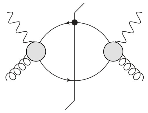 Figure 19
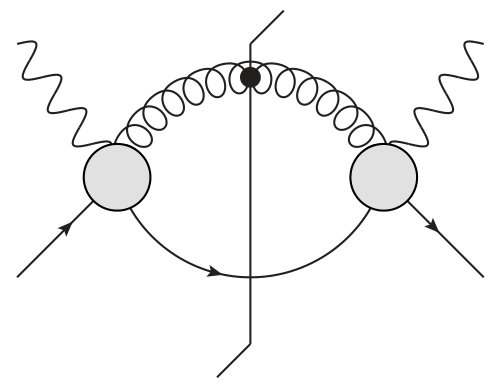 Figure 20
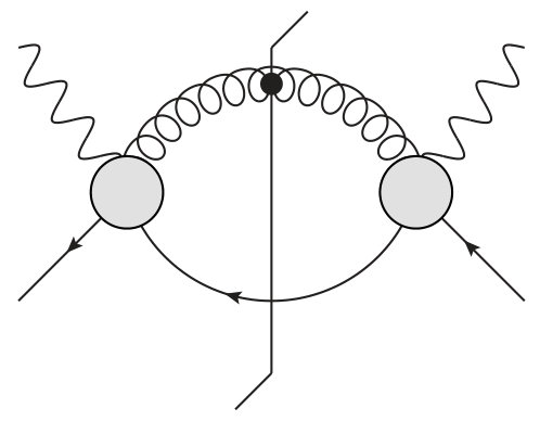 Figure 21
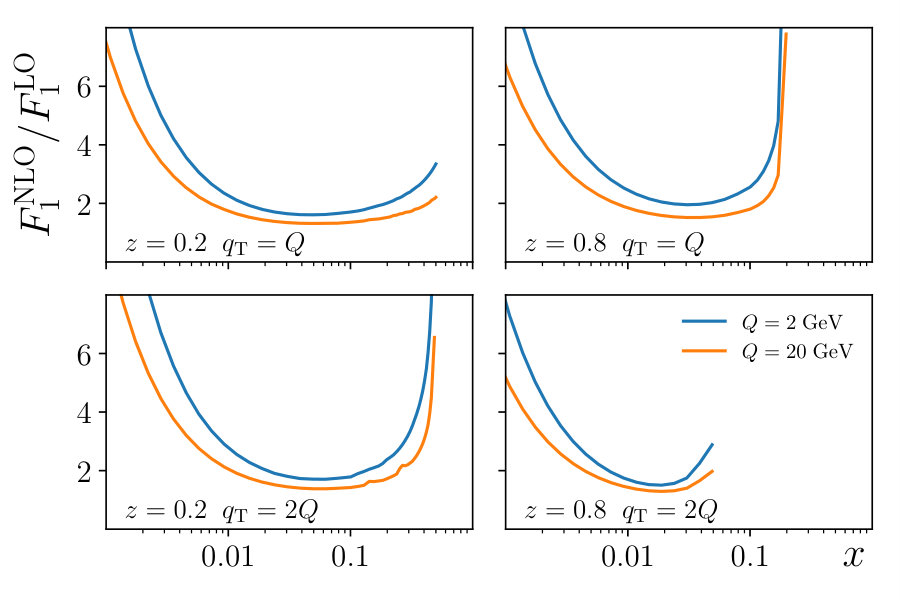 Figure 22
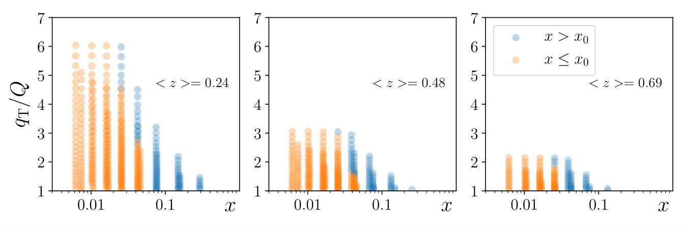 Figure 23
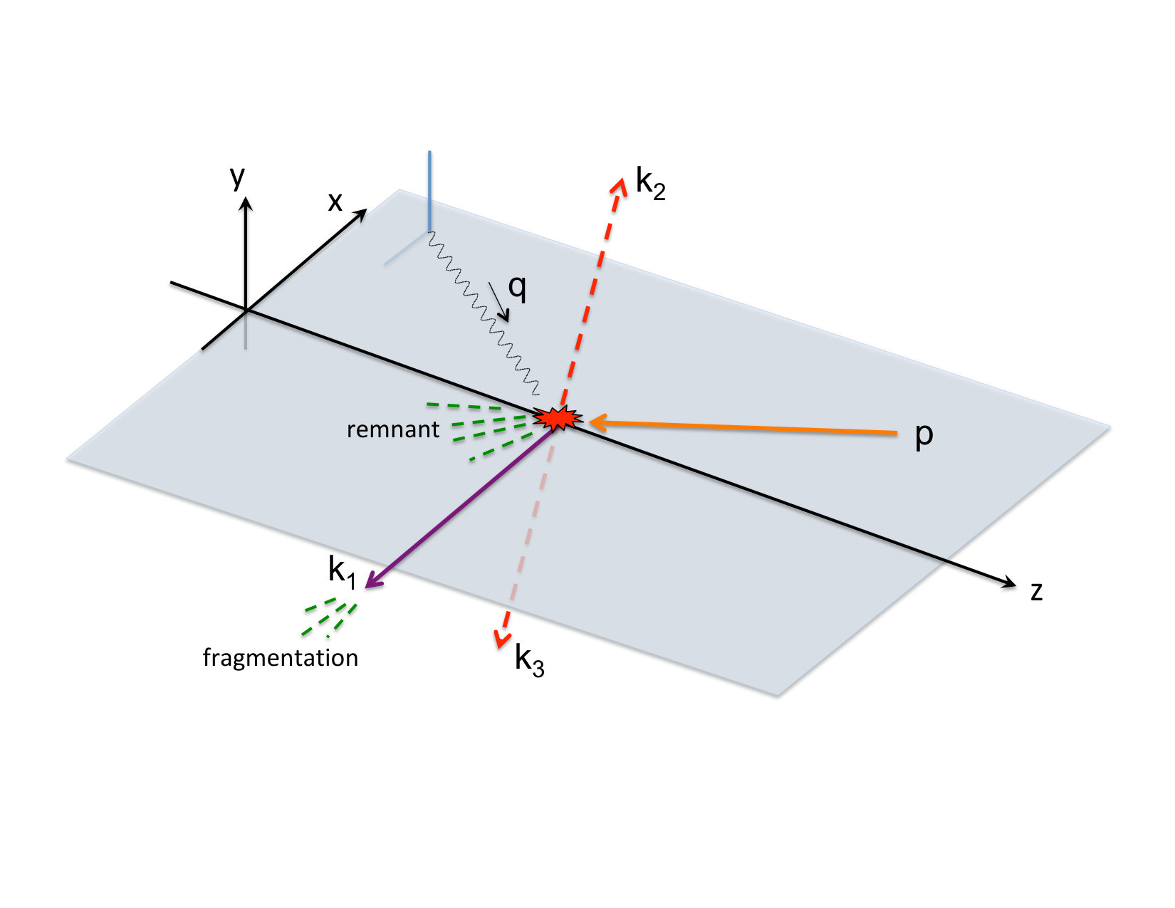 Figure 24
| virtual | real | combined | ||
|
|
||||
| N/A | ||||
| N/A | ||||
| N/A | ||||
| virtual | real | ||
| N/A | N/A | ||
| N/A | |||
| N/A | |||
Peer Reviews
No public reviews on file for this paper yet. If you reviewed it on a platform where reviews are public (OpenReview, ICLR, NeurIPS, ICML), you can paste yours below so the community can read it here.
Videos
No videos yet. Explain this paper in a talk, walkthrough, or lecture? Add one.
Large Transverse Momentum in Semi-Inclusive Deeply
Inelastic Scattering Beyond Lowest Order
B. Wang
Department of Physics, Old Dominion University, Norfolk, VA 23529, USA
Jefferson Lab, 12000 Jefferson Avenue, Newport News, VA 23606, USA
Zhejiang Institute of Modern Physics, Department of Physics, Zhejiang University,
Hangzhou 310027, China
J. O. Gonzalez-Hernandez
Department of Physics, Old Dominion University, Norfolk, VA 23529, USA
Jefferson Lab, 12000 Jefferson Avenue, Newport News, VA 23606, USA
Dipartimento di Fisica, Università di Torino, Via P. Giuria 1, 1-10125, Torino, Italy
T. C. Rogers
Department of Physics, Old Dominion University, Norfolk, VA 23529, USA
Jefferson Lab, 12000 Jefferson Avenue, Newport News, VA 23606, USA
N. Sato
Jefferson Lab, 12000 Jefferson Avenue, Newport News, VA 23606, USA
(4 March 2019)
Abstract
Motivated by recently observed tension between calculations of very large transverse momentum dependence in both semi-inclusive deep inelastic scattering and Drell-Yan scattering, we repeat the details of the calculation through transversely differential cross section. The results confirm earlier calculations, and provide further support to the observation that tension exists with current parton distribution and fragmentation functions.
††preprint: JLAB-THY-19-2897
I Introduction
In a previous article Gonzalez-Hernandez et al. (2018a), we discussed the semi-inclusive deep inelastic scattering (SIDIS) process:
[TABLE]
and we highlighted the challenge of finding agreement between calculations and existing SIDIS data in the very large transverse momentum transverse momentum limit where standard collinear factorization is expected to be valid. One motivation is that obtaining a description of the small transverse momentum behavior associated with nucleon structure requires a good understanding of the matching to large transverse momentum where a transverse momentum dependent (TMD) factorization description fails. Given the current focus on using deeply inelastic hadro-production to access nucleon structure sensitivity sensitivity, it is imperative to examine theoretical framework for the full -range in greater detail. In the language of Ref. Gonzalez-Hernandez et al. (2018a), we are interested in this paper in what was there called “region 3” behavior, corresponding to where is so large that the small approximations associated with TMDs are not reliable, but where ordinary collinear factorization should be applicable and reliable. Calculations to have existed for some time Daleo et al. (2005); Kniehl et al. (2005). The main observation of Ref. Gonzalez-Hernandez et al. (2018a) was that, while the correction gives an order of magnitude increase over the leading order, that still is not sufficient to achieve reasonable agreement with data for in the region of one to several GeVs, transverse momentum of order , and for moderate Bjorken-. Combined with similar observations concerning the Drell-Yan pointed out in Bacchetta et al. (2019), this points to general tension between transverse momentum dependent cross sections at and collinear factorization.
There are a number of potential explanations or solutions, including a direct re-tuning of collinear parton distribution and/or fragmentation functions to transversely differential SIDIS cross sections. (A proposal to constrain gluon PDFs in transversely differential Drell-Yan cross sections was made already in Berger et al. (1998).) But before proceeding to consider these directions, it is important to validate the in Daleo et al. (2005); Kniehl et al. (2005) that led to our conclusions in Gonzalez-Hernandez et al. (2018a). Therefore, we have in this paper repeated the large transverse momentum order calculation following a slightly different formal framework. We are able to reproduce the results in Daleo et al. (2005) very closely, thus bolstering the observations we made earlier in Gonzalez-Hernandez et al. (2018a).
The specific purposes of this article are as follows: i.) to lay out the logical steps of the calculation with enough detail, we hope, to lead to clues as to how to improve phenomenological agreement, ii.) to make available a convenient numerical implementation for the large region and, iii.) to present some quantitative results relevant to current experimental programs such as those at COMPASS and Jefferson Lab 12 GeV. Overall, our results support the general observations made in Gonzalez-Hernandez et al. (2018a).
In our calculations we use qgraf Nogueira (1993) to generate Feynman graphs and FORM Kuipers et al. (2013) to carry out spinor and color traces for the amplitudes. The renormalization counter terms are computed in MATHEMATICA with the packages FeynArts Kublbeck et al. (1990); Hahn (2001) and FeynCalc Mertig et al. (1991); Shtabovenko et al. (2016). Further analytic manipulations were performed in MATHEMATICA. The code to compute the cross sections are publically available at Gonzalez-Hernandez et al. (2018b).
In Sec. II, we explain our setup and notation. In Sec. III we summarize the organization of our calculations. This includes a classification of the partonic Feynman graphs needed at order and a discussion of the phase space integrals for multiparton final states. We discuss the results of the calculation in Sec. IV, and give concluding remarks in Sec. V.
II Notation and Conventions
We will express quantities in terms of the conventional kinematical variable . is the Breit frame transverse momentum of the produced hadron, and and are the four-momenta of the incoming target hadron and the virtual photon respectively. We will focus on the unpolarized and azimuthally-independent cross section since this is the most straight forward observable to calculate. (Although the results have potential implications also for polarization dependent observables.) Many general treatments of SIDIS as a process are available Meng et al. (1992); Levelt and Mulders (1994); Meng et al. (1996); Mulders and Tangerman (1996); Nadolsky et al. (1999, 2001); Barone et al. (2002); Ji et al. (2004); Bacchetta et al. (2004); Koike et al. (2006); Bacchetta et al. (2007, 2008). Our notation is consistent with trends among these, with modifications as needed for our current purposes.
The unpolarized differential cross section is
[TABLE]
or
[TABLE]
where is the unpolarized hadronic cross section. . The hadron transverse momentum is defined in a frame where the photon and incoming hadron are back-to-back (a “photon” frame). The Bjorken and the variable are the usual definitions and . is the usual leptonic tensor
[TABLE]
and is the hadronic tensor for SIDIS:
[TABLE]
where we have omitted spin and azimuthal angle dependent terms since we do not consider these in this paper. Also, we assume that and are small enough that both the proton and lepton mass can be dropped in kinematical and phase space factors. The normalization convention in Eq. (4) is so that the prefactor on the right hand side of Eq. (2) is similar to the unpolarized case.
The unpolarized structure functions and are defined by the usual gauge invariant decomposition
[TABLE]
Then, the cross section is
[TABLE]
In calculations, it is convenient to work with Lorentz invariant structure function extraction tensors with where
[TABLE]
Then,
[TABLE]
where in dimensions,
[TABLE]
(We we always use the massless target approximation – see discussion in Moffat et al. (2019).) It is useful to express transverse momentum in terms of
[TABLE]
In a frame where the incoming and outgoing hadrons are back-to-back, is the transverse momentum of the virtual photon (assuming, as always in this paper, that external hadron masses are negligible).
Our treatment of factorization will follow the general style of Collins (2011). The factorization theorem that relates the hadronic and partonic differential cross sections in SIDIS is
[TABLE]
The is from the partonic flux factor, and the 1 is from the conversion between and . The indices and denote, respectively, the flavors of the parton in the proton (with a momentum fraction ) and of the outgoing parton that fragments into hadron , whose momentum is a fraction of parton momentum. The incoming and outgoing parton momenta and satisfy and . (Indices and for incoming and outgoing partons and are not shown explicitly but are understood). and are the collinear parton distribution and fragmentation functions respectively. It is also useful to define partonic variables
[TABLE]
The differential partonic hard part in Eq. (11) is finite and well-behaved, and at large transverse momentum it starts at .
The unpolarized partonic structure tensor for scattering off parton into parton is defined in exact analogy with the hadronic tensor:
[TABLE]
with,
[TABLE]
Thus, from Eq. (11),
[TABLE]
The partonic structure function decomposition is
[TABLE]
Then,
[TABLE]
III Organization
III.1 Basic Setup
For a process with final state partons, and are squared amplitudes integrated over the -particle phase space for the outgoing partons,
[TABLE]
Here or is the squared amplitude for the process
[TABLE]
with the polarization sum of the virtual photon replaced by or . The subtraction terms in Eq. (19) are needed to remove double counting with lower orders of perturbation theory and cancel singularities in the first term. The form of the subtraction term will be discussed in Sec. III.2. It is assumed in Eq. (19) that all integrals that allow kinematical -functions to be evaluated have been performed. Also, the phase space factors associated with are excluded from the partonic phase space since they give the and dependence of the differential partonic cross section. The on the right hand side of Eq. (19) is the same factor in Eq. (4). The represents a generic phase space factor for scattering (see Eq. (35) and Eq. (39)).
Thus it is convenient to express the structure functions in the form
[TABLE]
where the is a sum over all possible partonic final states.
We will express the phase space in terms of Mandelstam variables:
[TABLE]
where , with the labeling in Fig. 1. For simplicity, and will be abbreviated as and from here on. All Mandelstam variables will refer to the partonic cross sections. Occasionally it will be useful to change kinematical variables, For example,
[TABLE]
The contribution to Eq. (19) is kinematically constrained to . At , only tree level processes contribute, and no singularities appear. At , soft, collinear and UV singularities arise as and poles in dimensional regularization with space-time dimension .
These singularities cancel in the sum of real, virtual and counterterm graphs and after applying collinear factorization. More discussion of the singularity structure at is available in Daleo et al. (2005); Arnold and Reno (1989). The partonic cross section is described in details in Nadolsky et al. (1999), and our results match that calculation. At , details below can also be found in, e.g., Aversa et al. (1989); Gordon and Vogelsang (1993); Ellis et al. (1980, 1983); Arnold and Reno (1989). The change of variables in Eq. (20) from momentum fractions to Mandelstam variables is
[TABLE]
where is replaced by , the virtuality of the spectator parton system. ( is in the notation of Gonzalez-Hernandez et al. (2018a)). Overall momentum conservation () gives
[TABLE]
The graphical structures needed at order can be classified as in Fig. 2. Each diagram corresponds to a contribution to the squared amplitude, and the blobs include all possible attachments. For the subprocesses, the blobs include up to one loop corrections in one side of the cut to give accuracy to the hard parts. The black dot marks the fragmenting parton and the other lines are integrated over all phase space.
The following are assumed and not shown explicitly in the graphs:
- •
Subtractions, consistent with factorization, for all collinear divergences.
- •
One QCD loop at all possible positions inside the blob in virtual processes.
- •
Associated UV counter term graphs for virtual processes.
Define the hard parts for individual graphs as
[TABLE]
where and . As before, and label incoming and fragmenting parton flavors respectively while and label the unobserved parton flavors. The graph is virtual when only one flavor index appears after the “;”. Figures 2(V-A) through 2(V-F) correspond to the graphs if all virtual loops in the blobs are removed.
So, for example, is represented by Fig. 2(R-A), when the partonic tensor is contracted with . Fig. 2(R-E) includes both and contributions where the prime indicates a different flavor. Note that graphs like Fig. 2(R-G) give contributions like or .
We work in the approximation that all particles are massless, except for the photon which is highly virtual, . In Eq. (19), for scattering,
[TABLE]
Thus the phase space factor is
[TABLE]
For the case, we follow the strategy in Ellis et al. (1980); Gordon and Vogelsang (1993) where we work in the rest frame of the system, in which
[TABLE]
where denotes unit vectors for the first components of the dimensional unit spatial vector in spherical coordinates. See Fig. 3.
In the center-of-mass of and , the spatial vectors , , , and are in the same plane. We then boost to the rest frame , where , and are still in the same plane – see Fig. 3. We choose the spatial orientations of this coordinate system so that , , and are in the plane created by the last two spatial axes. For these vectors, the first spatial components are zero. Then the scattering amplitudes do not depend on the first spatial components of or , and the 3-body phase space simplifies (see Appendix A for useful identities relating to the 3-body final state phase space). In this frame,
[TABLE]
where in the third equality we use that the scattering amplitudes are independent of the first spatial components of . That is,
[TABLE]
From overall momentum conservation
[TABLE]
Since can become zero in certain regions of and , dimensional regularization is needed for the behavior. Further details of the phase space are provided in the next subsection.
To summarize the basic steps, integrals for the unobserved final state phase space are first performed over angular variables. Then, integrals over momentum fractions are expressed via Eq. (29) as integrals over and . In the limit there are soft and collinear singularities, proportional to or , that cancel after combining and the corresponding virtual processes. There are additional collinear singularities in and virtual processes which are ultimately canceled by subtraction terms in the factorization algorithm. (These contain also and plus distributions.) All contributions are integrated over the physical range of in Eqs. (29)–(32).
III.2 Factorization Order-By-Order
Once all real and virtual Feynman graphs have been computed in dimensional regularization, they must be combined in an algorithm consistent with a factorization theorem.
According to the collinear factorization theorem, hard factors are independent of the species of target and final state particles, so hard scattering calculations can be performed for free and massless partons as the target and final state without loss of generality. (In other words, we will consider perturbatively calculable parton-in-parton PDFs and and parton-to-parton FFs.) This simplifies calculations, so we start our calculations by rewriting Eq. (15) as a factorization theorem for a partonic initial and final state:
[TABLE]
All manipulations will be done in dimensions until the very end. The left side is now an argument of , , and , and the PDFs and FFs have subscripts and . The momenta and play the roles that and played earlier. The initial has a flavor and the final has a flavor . The second line in Eq. (41) defines the “” notation as the usual shorthand for the convolution integrals in and . On the last line, and are hadronic tensors calculated to LO and NLO in the hard parts, i.e. what one normally means when one speaks of a “leading order” or “next-to-leading order” calculation in collinear pQCD.
Expanding Eq. (41) to the relevant order in gives
[TABLE]
The aim is to get the hard parts, and . The leading order is just
[TABLE]
where the expression for is simple and well-known – it is just the sum of tree level graphs contributing to .
To get , first write
[TABLE]
The term in braces is the correction to the leading order so it vanishes by construction at order in the hard part. Also, it contains subtractions for the overlap with the LO, so it is infrared safe through order in hard scattering. Thus, we may rewrite it as:
[TABLE]
The term in braces on the second line is equal to the first line evaluated with hatted partonic variables and expanded only to order in the coupling. Comparing with Eq. (42) and Eq. (44) shows that the factor in braces in Eq. (45) is . We use Eq. (43) to evaluate it explicitly in terms of low order PDFs and FFs:
[TABLE]
Here, the is the sum of order graphs contributing to without any subtractions (i.e., graphs in Fig. 2(R-A) through Fig. 2(V-F) integrated over phase space, but absent the subtractions). The second two terms are obtained from Eq. (43), expanded to order . The last line in Eq. (46) uses the known results for PDFs and FFs calculated to for massless quarks and gluons:
[TABLE]
Note that, consistent with the scheme, the renormalized order PDFs and FFs in dimensional regularization for massless pQCD are just poles. There are no factors or logarithms of . Thus the last line of Eq. (46) involves no factors of . For completeness, the one-loop splitting functions Altarelli and Parisi (1977) are
[TABLE]
Our calculations need Eq. (46), contracted with specific tensors. The substraction scheme has been carry out without contracting the Lorentz indices of the partonic tensor. However the method is equally applicable for any kind of contraction with external momenta. In our calculations we carry out the substractions separately for the two extraction tensors in Eq.(7) and verified analytically the cancellation of all infrared and collinear singularities.
IV Results
IV.1 Combining real and virtual contributions
After the hard real and virtual contributions are calculated, they must be combined into infrared safe squared amplitudes. Table 1 shows graphs from corresponding real and virtual processes. Note that the correspondence between real and virtual processes is not one-to-one. In particular, infrared (soft and collinear) singularities in are canceled by three real processes. A subtlety arises when a quark loop appears on the gluon leg of . This creates a collinear pole term proportional to , the number of massless quark flavors in the loop. This pole term is canceled after adding the real processes and with all massless flavors (other than ) Gordon and Vogelsang (1993). For processes with a non-spectator gluon leg, the dependence of the collinear pole is removed by factorization. Also notice that some real processes have no corresponding virtual ones, and in these cases factorization subtractions are sufficient to remove all infrared poles. Since many graphs need to be combined, the results are presented as the six scattering hard parts listed in the last column of Table 1. We also need the hard parts for processes with reversed quark number flow in one or two open fermion lines in the graph. That is, in one or two open quark lines, quarks and their corresponding anti-quarks are interchanged. These are easily related to the hard parts already listed in Tabel 1 by using the fact that QED vertices acquire a minus sign under charge conjugation. The results are summerized in Tabel 2. Note that when a quark line links an outgoing spectator quark anti-quark pair, there is no need for the reversed quark flow. This is because the spectator momenta are integrated over and interchanging the quark and anti-quark will double count the contribution.
IV.2 Comparison with existing results
After combining the graphs in each of the six scattering channels in Table 1, we have verified explicitly that all single and double poles cancel. The terms left are finite in the limit , and constitute the infrared safe hard parts in the last column of Table 1. As a check, we have compared with a (privately obtained) computer calculation that appears to reproduce the results of Ref. Daleo et al. (2005) but is modified to be consistent with the kinematics of the current experimental data. For most kinematics, the calculations agree within experimental uncertainties, but we found several possible differences.
- •
In the last row of Table 1, our calculation of terms from the projection with the charge structure and differs from the corresponding terms calculated in the previously existing code by a minus sign. (By contrast, terms with agree.)
- •
As is discussed in subsection IV.1, adding the real processes and with all massless flavors gives terms proportional to . The pole parts of these terms are canceled by the corresponding poles from . However, a finite part remains since the real processes above with final state quark pairs give identical contribution even when the quark pairs are not collinear. These terms contribute to the third row of Table 1. In the previously existing code, we did not find an explicit dependence on in this channel.
The numerical result of our calculation can in some cases differ from the previously existing code by as much as for certain individual subchannels. In the kinematics of the COMPASS experiment, this translates into a discrepancy of up to for the overall cross section.
IV.3 Phenomenological Results
We examine the impact of the corrections in SIDIS by plotting the NLO to LO ratio -factor for the structure function. We will consider values of between and since this is a region where factorization theorems based on current fragmentation in SIDIS is conventionally expected to apply.
For , , , we choose values of , and , which correspond to kinematics ranges accessible by existing experimental facilities such as COMPASS and JLab 12. Fig. 4 shows the -factor across the aforementioned kinematical range, and it shows a clear concave up shape in its dependence on with values that decrease as varies from to GeV.
It is notable that even for as large as GeV, the -factor is greater than , even at its minimum value. Note also that this minimum is approximately in the region of , close to the valence region relevant to many hadron structure studies. The -factor increases at smaller values of , indicating that the NLO corrections becomes increasingly important for describing regions with large . It also increases at large until it reaches the kinematic boundary where the phase space for the hadron production vanishes.
The enhancements at large can be traced to the logarithms of (see Eq. 32 and appendix D) which are associated with soft gluon effects near the kinematical threshold. Thus it is likely that threshold resummation becomes important in this region. Point-by-point in , effects near the kinematical boundaries are more apparent than in -inclusive cross sections. It is interesting to compare with observations found in Anderle et al. (2013) where threshold resummation effects for integrated SIDIS were found to give sizable corrections, but not the factor of enhancement needed to explain the largest present in Fig. 4.
The minimum in the -factor is helpful for identifying regions in where ordinary fixed order treatments are most likely to be sufficient. Given a set of values for , , and , let denote the value corresponding to the minimum -factor. Then bins in , , , can be classified according to and . We show this in Fig. 5 for kinematical bins corresponding to recent COMPASS -dependent SIDIS multiplicities Aghasyan et al. (2018) for . The values of the for which the -factor reaches its minimum for can be read from the plots. Away from these regions, additional resummation techniques may be needed.
It may also be necessary to update collinear PDFs outside these regions in order to fully describe the large behavior. As mentioned in Gonzalez-Hernandez et al. (2018a), the large tails of SIDIS are sensitive to the large PDFs and large FFs. These could potentially open up new opportunities to constrain collinear PDFs at large momentum fractions.
At the same time, factorization theorems for the full -dependent SIDIS spectrum, including with non-perturbative TMD PDFs and TMD FFs, need the large component in order to have a completely reliable tests of the factorization formalism. Ideally, such validation will take place when -dependent SIDIS data are included in the simultaneous extraction of collinear PDFs and FFs as well as non-perturbative TMD PDFs and FFs in QCD global analysis.
V Conclusion
The computational tools necessary to reproduce Fig. 4, Fig. 5 and other similar calculations are available at Gonzalez-Hernandez et al. (2018b), along with documentation. As indicated in the introduction, these generally confirm earlier calculations (e.g., Daleo et al. (2005); Kniehl et al. (2005)) of the overall cross section to within about , well within present experimental uncertainties, and thus strengthens our earlier position Gonzalez-Hernandez et al. (2018a) that significant tension exists between existing SIDIS data and collinear factorization calculations at large .
We have identified region where collinear factorization appears most reliable as the regions with minimal -factors, with current sets of collinear PDFs and FFs. As discussed in Sec. IV.3, minimal values for the -factor lie in the region , that is, approximately in valence kinematics. The increase of the -factor at both smaller and larger values of , may point at the importance of resummation effects outside the valence region, or the need to refit collinear PDFs and FFs. This last interpretation is consistent with that of our previous study Gonzalez-Hernandez et al. (2018a). It is also important to note that the kinematics of the contribution places severe kinematical constraints on the relationship between the initial and final state partons. Therefore, it is likely that the generally large -factors are at least partly due simply to a kinematical suppression of the contribution, and are not a fundamental problem with the convergence of the perturbation series. We note that Reference Balitsky and Tarasov (2018) has addressed somewhat similar issues, but in the region where is still small enough that a power expansion is still meaningful, and also in the limit of .
As a next step, we plan to refit collinear functions in the large region, using SIDIS and -annihilation to back-to-back, and Drell-Yan scattering to explore the possibility that this allows the region of minimum -factor in Fig. 4 to be fully accommodated with minimal modification to existing fits.
Since the pioneering work in presented in Meng et al. (1996); Graudenz (1997); Nadolsky et al. (1999), there has been a large number of studies on unpolarized SIDIS cross sections Koike et al. (2006); Anselmino et al. (2007, 2014); Signori et al. (2013); Sun and Yuan (2013); Sun et al. (2014); Bacchetta et al. (2017). Unpolarized SIDIS is however, only one component in a broad program of phenomenolical studies where the universality of parton correlation functions plays a central role in testing pictures of nucleon structure Anselmino et al. (2017, 2015); Bacchetta et al. (2015); Scimemi and Vladimirov (2018); Kang et al. (2017, 2015a); Landry et al. (2003); Sun et al. (2017, 2011); Echevarria et al. (2015); Guzzi et al. (2014); Echevarria et al. (2016, 2014); Boglione et al. (2018, 2017); Kang et al. (2015b); Lin et al. (2018); Ye et al. (2017); Bacchetta et al. (2019); Bastami et al. (2018); Bertone et al. (2019). In order for this program to be successful, the precision in the determination of parton correlation functions needs to meet the demands of the increasingly precision of current and future experimental programs Airapetian et al. (2013); Adolph et al. (2013, 2017); Seidl et al. (2019); Aschenauer et al. (2019); Bradamante (2018). This demands a satisfactory resolution to problems in the region for which the pQCD calculation at large is crucial.
Acknowledgements.
We thank J. Owens, J.-W. Qiu, and W. Vogelsang for very useful discussions. We thank R. Sassot for explanations regarding the code in Daleo et al. (2005). T. Rogers’s work was supported by the U.S. Department of Energy, Office of Science, Office of Nuclear Physics, under Award Number DE-SC0018106. This work was also supported by the DOE Contract No. DE- AC05-06OR23177, under which Jefferson Science Associates, LLC operates Jefferson Lab. N. Sato was partially supported by DE-FG-04ER41309, DE-SC0018106 and the DOE Contract No. DE- AC05-06OR23177, under which Jefferson Science Associates, LLC operates Jefferson Lab. B. Wang was supported in part by the National Science Foundation of China (11135006, 11275168, 11422544, 11375151, 11535002) and the Zhejiang University Fundamental Research Funds for the Central Universities (2017QNA3007). J. O. Gonzalez-Hernandez work was partially supported by Jefferson Science Associates, LLC under U.S. DOE Contract #DE-AC05-06OR23177 and by the U.S. DOE Grant #DE-FG02-97ER41028.
Appendix A Identities for three-body partonic phase space
The phase space of three massless particles has the form
[TABLE]
The integral can be performed in the center-of-mass frame of and
[TABLE]
where denotes the first components of the dimensional unit spatial vector in spherical coordinates, and
[TABLE]
In phase space, and are related with observables. The “azimuthal” angles in can be integrated to give
[TABLE]
where is the dimensional angular volume,
[TABLE]
and are related to Lorentz invariants and via
[TABLE]
In terms of and , the phase space becomes
[TABLE]
To simplify the and phase space, we work in the and center-of-mass frame where and take the form of Eqs. (36) and (37). The choice of the spatial orientation of axes also follows the discussion below Eq. (36). In this frame
[TABLE]
Since the scattering amplitudes are independent of the first spatial components of , the “azimuthal” part of can be integrated to give
[TABLE]
Appendix B Phase space integration for processes in SIDIS
The main effort of the calculation is in the 2 3 process . After partial fractioning (to be discussed Appendix D), each term from the squared amplitudes , in Eq. (38) contains at most two Mandelstam variables depending on the angles and . So, up to overall factors, Eq. (38) takes the form
[TABLE]
where and are integers. The coefficients , , , , and are specific to the squared amplitude and do not depend on and . They are determined by the spatial orientations of axes in the rest frame. Note that Eqs. (36)–(37) do not determine uniquely the components of , , and . There can still be a rotation in the plane determined by the last two spatial axes. Taking advantage of this freedom, we specify three frames.
- Frame 1:
[TABLE]
- Frame 2:
[TABLE]
- Frame 3:
[TABLE]
where
[TABLE]
There are three cases (see Appendix C for a proof) for the coefficients in the integral in Eq. (67): (1) and ; (2) and ; (3) and . Integrals in case (3) can be transformed to case (2) by switching to another frame. With multiple frames, the number of integrals to compute can be reduced. In the following we show how the integrals in case (1) and (2) are obtained.
[TABLE]
where for simplicity an overall factor is not shown and we choose , , and . In the frames we choose above, can be or . Here the signs of the trigonometric function terms in the denominator are chosen to be negative. All other choices can be transformed to this one by applying substitutions , and/or . The derivation of this integral can be found in appendix A of van Neerven (1986).
- Case (2): In this case the integral no longer has a closed form. Following steps similar to appendix A of van Neerven (1986), we arrive at
[TABLE]
where . The integral representation of hypergeometric function is used. Note the notation for integrals with different denominator structures. The result of evaluating Eq. (85) for specific and is given in Appendix F. Here can be or . The remaining integral has to be performed by expanding the integrand into series of , and computing the integral order by order. The subtlety comes from the treatment of the factor , which can produce poles for . The integral has the form
[TABLE]
where is a regular function at . When , the pole term can be made explicit using the identity
[TABLE]
where the “plus” functions are defined, for a function , through
[TABLE]
When , the integral in Eq. (87) is divergent. Nonetheless, it can be analytically continued. To do this, we write
[TABLE]
Note that, in the first term on the right-hand side of Eq. (90), the power of is increased by 1, with a regular function . The second term is divergent, but can be analytically continued using functions:
[TABLE]
The manipulation in Eq. (90) can be repeated until the power of in the integral becomes , in which case Eq. (88) can be used. To expand the hypergeometric function in the integrand in Eq. (85), we note that if either or is less than 1, the hypergeometric series terminates and the function reduces to a polynomial. For and we use the expansion
[TABLE]
For the case that one of and is larger than 1 and the other is at least 1, we use Gauss’s contiguous relations to reduce or . For example, for and (with the shorthand notation ), we use
[TABLE]
to get
[TABLE]
Other well-known non-trivial aspects of the computation are the conversion of the expressions in the squared amplitude into forms that allow Eq. (84) or Eq. (85) to be used, which are reviewed in Appendix D, and the algorithm for calculating virtual corrections, which are reviewed in Appendix E. Finally the procedure for combining all Feynman graph calculations consistently into a a factorized cross section is reviewed in Appendix LABEL:a.subtraction.
Appendix C Proof that and in Eq. (67)
First, we show that . In the center-of-mass frame of and ,
[TABLE]
where . can be any one of , , with the subscript suppressed above. In this frame, and
[TABLE]
The are Lorentz invariants and thus holds in any frame. Since the signs of do not change and
[TABLE]
we conclude that and , where the “” holds when the corresponding variable is or , and the “” holds for .
Appendix D Partial fraction algorithm
To perform the three-body phase space integrations as described Sec. B, it is necessary to first convert expressions in the squared amplitude into forms that allow Eq. (84) or Eq. (85) to be used. In this appendix, we review the way this can be automized.
To simplify the discussion, we will refer to angle dependent Mandelstam variables (ADMV):
[TABLE]
The angle independent Mandelstam variables (AIMVs) are:
[TABLE]
A general term in the squared amplitude starts as simple products of AIMVs and ADMVs. A conversion to a useful form is accomplished with a set partial fractions such that each term in the squared amplitude can be expressed as
[TABLE]
with and being real numbers that could be positive, negative or zero. The quantity in the brackets is some combination of the AIMVs while and are two different types of ADMV that belong to to either , or . A term in such a form is called a “reduced” term. Otherwise, we will call it “unreduced”. Example are:
- •
reduced** terms**: (constant), (), (),()
- •
unreduced** terms**: (), (), ()
We need the following further sets of definitions:
- •
t-type, u-type, s-type Mandelstam variables: An ADMV is referred to as t-type if it is or , and similarly for u-type and s-type.
- •
The ADMVs are not independent variables; it is possible to construct linear relations relating them. This is achieved by squaring different rearrangements of the momentum conservation equation:
[TABLE]
- Two ADMV relations (2ARs): One such type of relation is between two ADMVs of the same type. These are obtained by moving one of , , and in Eq. (110) to the right-hand side and squaring the equation. For instance, moving to the right and squaring gives
[TABLE]
relating two u-type ADMVs. Similarly, moving or to the right gives the relations for -type or -type ADMVs respectively. There are three 2ARs. The other two are:
[TABLE]
- Three ADMV relations (3ARs): Another type of relation is between three ADMVs, each from a different ADMV type. We can get such relations for any three ADMVs of different types. To do this notice that exchanging the positions of or with in Eq. (110) and squaring will give one of such relation. For instance, squaring :
[TABLE]
a relations between , , and . After one such relation is obtained, the others are obtained by replacing the ADMVs in that relation using three 2ARs.
Now the partial fraction is implemented in two steps:
-
Step 1: Consider a term in the squared amplitude. The first step is to reduce the number of ADMVs in the denominator to two or fewer, and to ensure that no two ADMVs of the same type appear in the denominator. This is done in two substeps:
-
Substep 1: First, separate any ADMVs of the same type in the denominator. If two ADMVs of the same type appear in the denominator of , use a 2AR for the two ADMVs to write a factor of unity in the form
[TABLE]
and write
[TABLE]
with . Expanding the right side of Eq. (116) produces a sum of new terms. Each will have one power lower of these two ADMVs in its denominator. Further multiplication by unity factors like Eq. (115) can be repeated until in all terms only one of the two ADMVs appears in any denominator. As an example, consider
[TABLE]
and both appear in the denominator, so we will use Eq. (113) to write Eq. (115):
[TABLE]
Then
[TABLE]
- Substep 2: After Substep 1 is done for all three types, the leftover terms have denominators with at most three ADMVs, all from different types. For terms with two or fewer ADMVs in the denominator, nothing more needs to be done in this step. For terms with three ADMVs in the denominator, one may write a 3AR in the form of Eq. (115) and reduce the number of ADMVs in the denominator to two or fewer in a way similar to Substep 1. For example, say that
[TABLE]
Then it is possible to eliminate , and by using Eq. (114) to construct Eq. (115). Then,
[TABLE]
- Step 2: After Step 1 is completed, all terms have two or fewer ADMVs in the denominator. To get to the final form in Eq. (109), we need to make sure no third ADMV appears in the numerator. This is done by noticing that the ADMVs in the numerator can be written in terms of the ADMVs of the denominator using 2ARs and 3ARs. For instance, if one term has in the denominator, then any t-type ADMV in the numerator can be replaced by , and u-type by , using 2ARs. Any s-type ADMV can be replaced by a linear combination of and using the corresponding 3AR involving and . This puts in the form of Eq. (109). (Recall that and can be negative or zero.) This example had two ADMVs in the denominator. If the number of ADMVs in the denominator is 1, one can express the ADMVs in the numerator in terms of two ADMVs of different types, where one is the ADMV in the denominator and the other is chosen randomly. If the number of ADMVs in the denominator is 0, then the ADMVs in the numerator can be expressed by any two randomly chosen ADMVs of different types. There are six ADMVs, but the four relations from Eqs. (111)–(114) eliminate four in terms of the other two.
Appendix E Virtual Contributions
At order , virtual corrections to the partonic cross section involve only one-loop integrals. Comprehensive reviews of the methods for this type of calculation can be found in Berger and Forde (2010); Britto (2011); Ellis et al. (2012). In this article, we use the traditional Passarino-Veltman (PV) approach Passarino and Veltman (1979), for which we closely follow the notation of Ellis et al. (2012).
Our virtual contributions are the interference terms between tree-level amplitudes and amplitudes with an additional virtual loop, averaged(summed) over initial(final) states. The structure of each such interference term is
[TABLE]
The denominators contain massless propagators of the form , where depends only on external momenta, which we will call . That is, or combinations thereof. The trace in (123) contains Dirac gamma matrices contracted with either the external momenta , or with the loop momentum . Both IR and UV divergences are handled by standard dimensional regularization techniques. After these steps, the numerator in Eq (123) is a collection of terms with Lorentz invariant products of loop and external momenta. All integrals needed to calculate the virtual corrections in Figure 2 can be written in one of the following ways:
[TABLE]
where higher rank integrals cannot appear since, in every case, virtual correction diagrams at one-loop involve at least one gluon propagator. We have left the Feynman prescription implicit in the denominators in Eq. (124), and partonic cross section calculations are done in massless QCD. These tensor integrals can be written in terms the scalar box (), triangle () and bubble () integrals using the Passarino-Veltman reduction procedurePassarino and Veltman (1979).
As an example, consider the steps to reduce . Symmetry properties allow , and to be written in terms of form factors , , , and :
[TABLE]
Defining the Graham matrix and the row vectors , , the contraction of both sides of Eq. (125c) with and respectively gives
[TABLE]
where is defined by the relations
[TABLE]
Here we have used the notation . The results for above are obtained by contracting with the right-hand side of Eq. (125c) and using the property that the products can always be written in terms of the denominators as
[TABLE]
This allows to be reduced to rank-1 integrals, whereupon expansion according to Eqs. (125b), lead to Eqs. (E). Solving Eq. (126) gives and in terms of form factors corresponding to lower rank tensor integrals. In a similar way, one may reduce residual and form factors so that only the scalar integrals and appear at the end of the reduction procedure. Equations analogous to (126) and (E) for all cases in Eq. (124) are provided in Appendix A of Ellis et al. (2012).
After the reduction procedure, all virtual contributions from Figure 2 are in terms of scalar integrals, whose values depend only on Lorentz invariants constructed from momenta that appear in the denominators. The complete set of scalar integrals are in Ellis and Zanderighi (2008). In our calculation, all of these contain single or double pole singularities.
The singular behavior of and corresponds to soft and collinear divergences that exactly cancel the soft and collinear singularities in the calculation of the corresponding channel.
For our computations, we only need expressions for a reduced number of cases for and , following the notation of Ellis and Zanderighi (2008): divergent type 1 and type 2, divergent type 2
The usual UV singularities introduced by virtual corrections ultimately are all produced by -type integrals. UV divergent tadpole integrals also appear but are zero in a massless theory. Thus, keeping track of integrals accounts for all UV singularities, which cancel in the sum of virtual graphs. Self-energy diagrams on external legs enter for each channel via the corresponding factors of field strength normalization , as prescribed by the LSZ theorem.
At order , deviates from unity only for partonic scattering. Denoting the sum of amputated diagrams for leading order, virtual, and real emission by , and , the square-modulus amplitude for partonic scattering is
[TABLE]
Explicit solutions for scalar integrals given in Ellis and Zanderighi (2008) hold when all of the relevant Lorentz invariants are space-like. When needed, we perform analytic continuation on the logarithms, by restoring the Feynman prescription . For the dilogarithms in our calculation, we find the following relation useful
[TABLE]
where both and are positive.
Appendix F Angular integrals with a virtual photon
For completeness we provide a complete list of the relevant angular integrals. The method to compute these integrals is described in detail in Sec Sec. B. The alternatives for some of the integrals here can be found from appendix C of Ref. Beenakker et al. (1989). But there the list of integrals is computed for heavy quark production process and is not adequate for SIDIS. To compactify notation, we define
[TABLE]
The integrals are computed up to the needed powers in . The expressions for from Eq. 85 needed for order SIDIS are then
[TABLE]
Certain order terms are not needed and may be dropped in calculations at .
The reference list from the paper itself. Each links out to its DOI / PubMed record.
- 1Gonzalez-Hernandez et al. (2018 a) J. O. Gonzalez-Hernandez, T. C. Rogers, N. Sato, and B. Wang, Phys. Rev. D 98 , 114005 (2018 a) , ar Xiv:1808.04396 [hep-ph] . · doi ↗
- 2Daleo et al. (2005) A. Daleo, D. de Florian, and R. Sassot, Phys. Rev. D 71 , 034013 (2005) , ar Xiv:hep-ph/0411212 [hep-ph] . · doi ↗
- 3Kniehl et al. (2005) B. A. Kniehl, G. Kramer, and M. Maniatis, Nucl. Phys. B 711 , 345 (2005) , [Erratum: Nucl. Phys.B 720,231(2005)], ar Xiv:hep-ph/0411300 [hep-ph] . · doi ↗
- 4Bacchetta et al. (2019) A. Bacchetta, G. Bozzi, M. Lambertsen, F. Piacenza, J. Steiglechner, and W. Vogelsang, (2019), ar Xiv:1901.06916 [hep-ph] .
- 5Berger et al. (1998) E. L. Berger, L. E. Gordon, and M. Klasen, Phys. Rev. D 58 , 074012 (1998) , ar Xiv:hep-ph/9803387 [hep-ph] . · doi ↗
- 6Nogueira (1993) P. Nogueira, J. Comput. Phys. 105 , 279 (1993) . · doi ↗
- 7Kuipers et al. (2013) J. Kuipers, T. Ueda, J. A. M. Vermaseren, and J. Vollinga, Comput. Phys. Commun. 184 , 1453 (2013) , ar Xiv:1203.6543 [cs.SC] . · doi ↗
- 8Kublbeck et al. (1990) J. Kublbeck, M. Bohm, and A. Denner, Comput. Phys. Commun. 60 , 165 (1990) . · doi ↗