A Resolution Study of Magnetically Arrested Disks
Christopher J. White, James M. Stone, Eliot Quataert

TL;DR
This study examines the numerical convergence of simulations of magnetically arrested disks around spinning black holes, finding some flow properties converge while small-scale turbulence and emission variability do not.
Contribution
It provides a detailed analysis of convergence in GRMHD simulations of black hole accretion disks using Athena++, highlighting which aspects are reliable and which require higher resolution.
Findings
Accretion rate and large-scale flow structure are converged.
Jet energy and spin energy extraction efficiency are converged.
Small-scale turbulence and emission variability are not fully converged.
Abstract
We investigate numerical convergence in simulations of magnetically arrested disks around spinning black holes. Using the general-relativistic magnetohydrodynamics code Athena++, we study the same system at four resolutions (up to an effective 512 by 256 by 512 cells) and with two different spatial reconstruction algorithms. The accretion rate and general large-scale structure of the flow agree across the simulations. This includes the amount of magnetic flux accumulated in the saturated state and the ensuing suppression of the magnetorotational instability from the strong field. The energy of the jet and the efficiency with which spin energy is extracted via the Blandford-Znajek process also show convergence. However the spatial structure of the jet shows variation across the set of grids employed, as do the Lorentz factors. Small-scale features of the turbulence, as measured by…
Click any figure to enlarge with its caption.
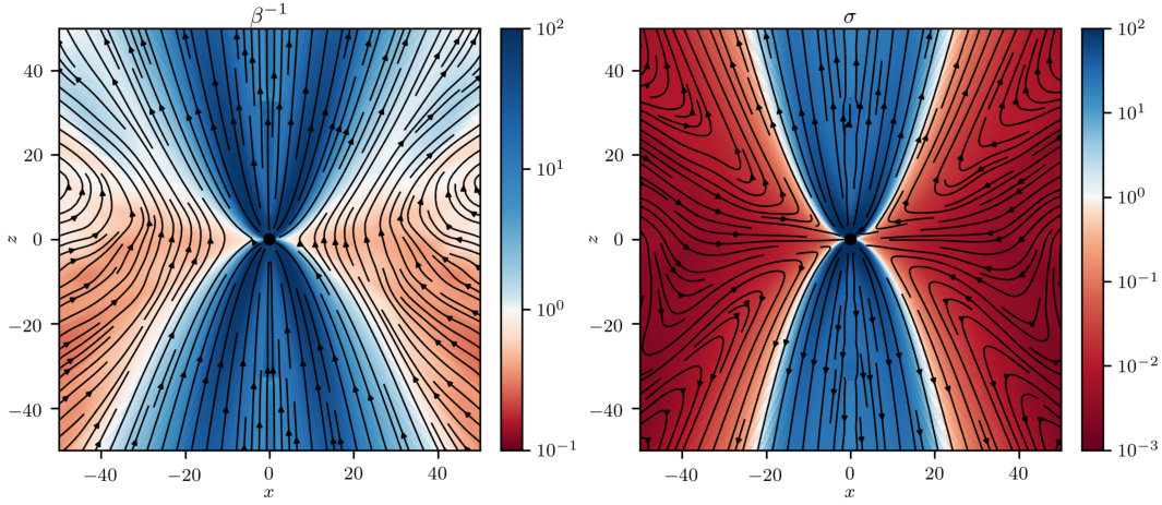 Figure 1
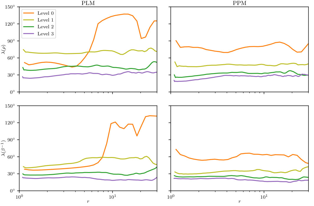 Figure 2
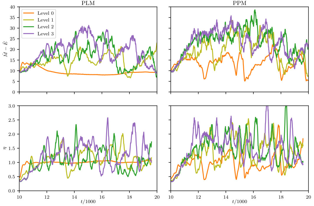 Figure 3
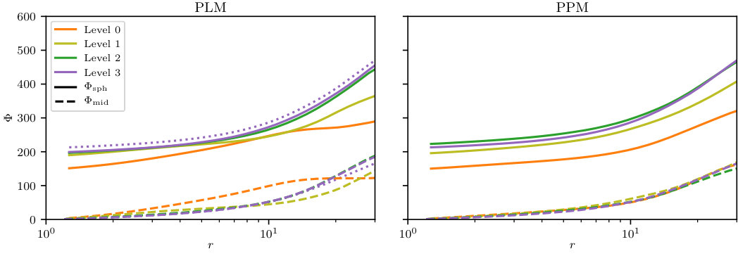 Figure 4
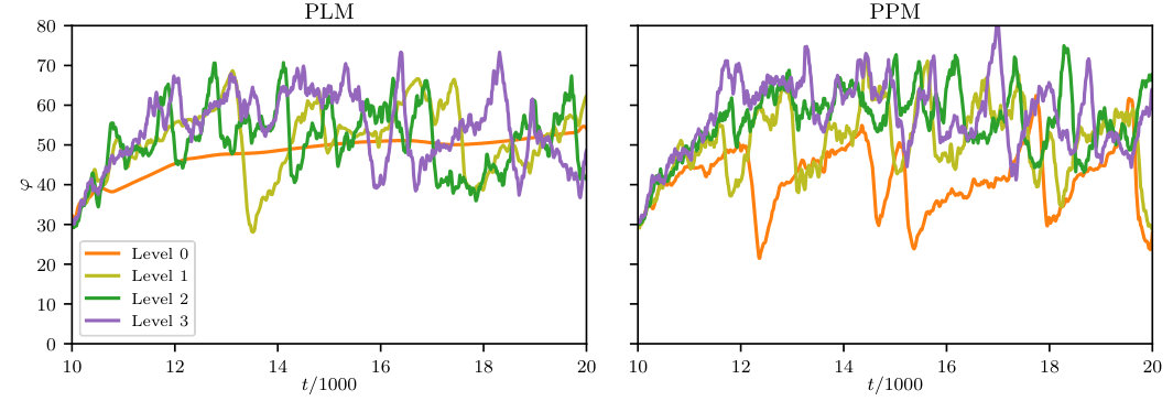 Figure 5
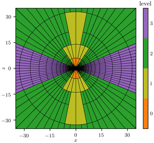 Figure 6
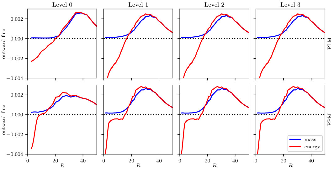 Figure 7
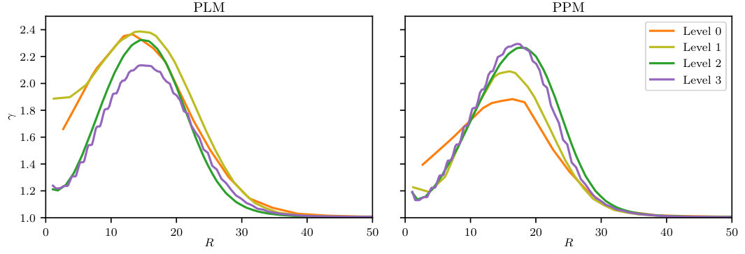 Figure 8
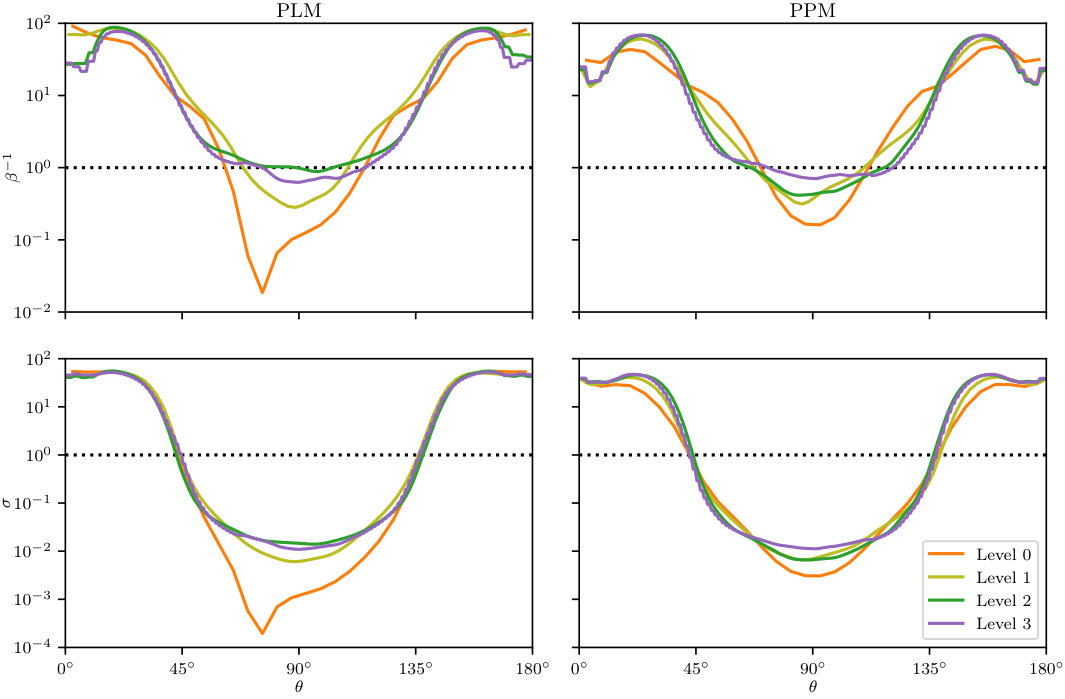 Figure 9
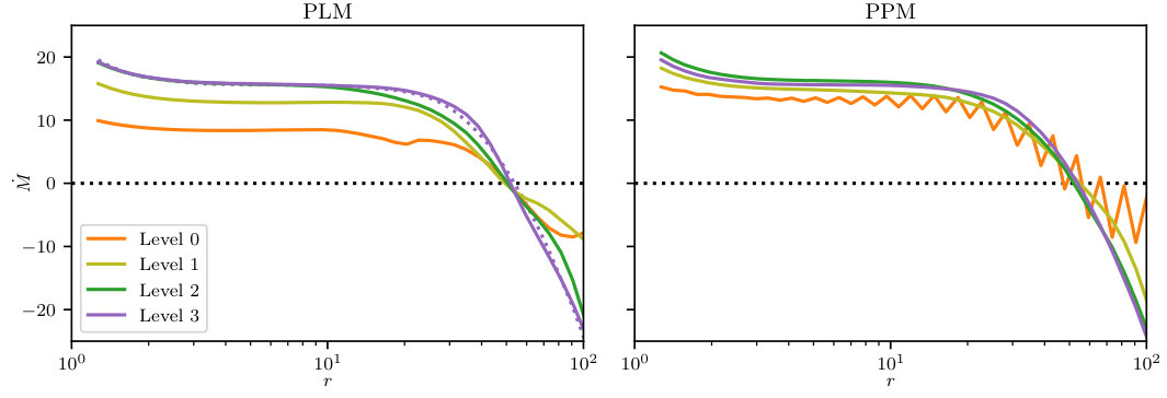 Figure 10
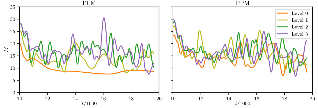 Figure 11
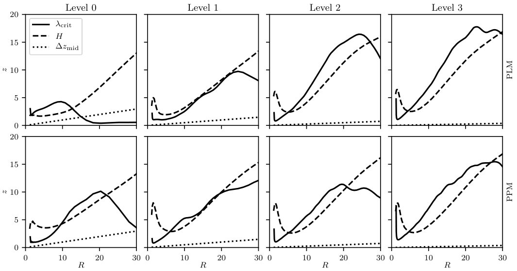 Figure 12
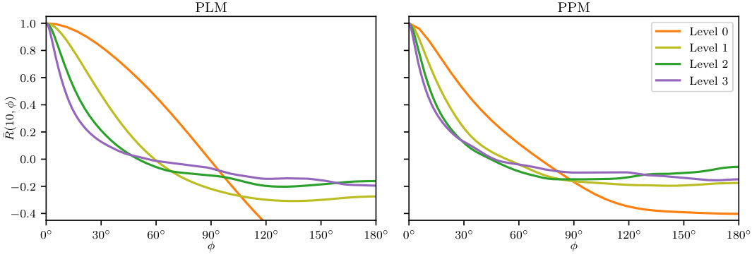 Figure 13
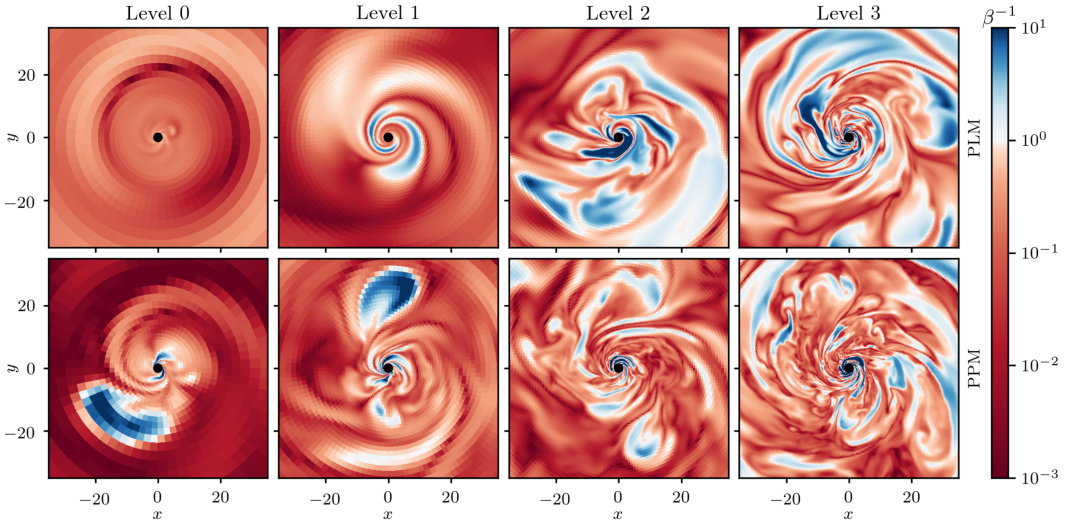 Figure 14
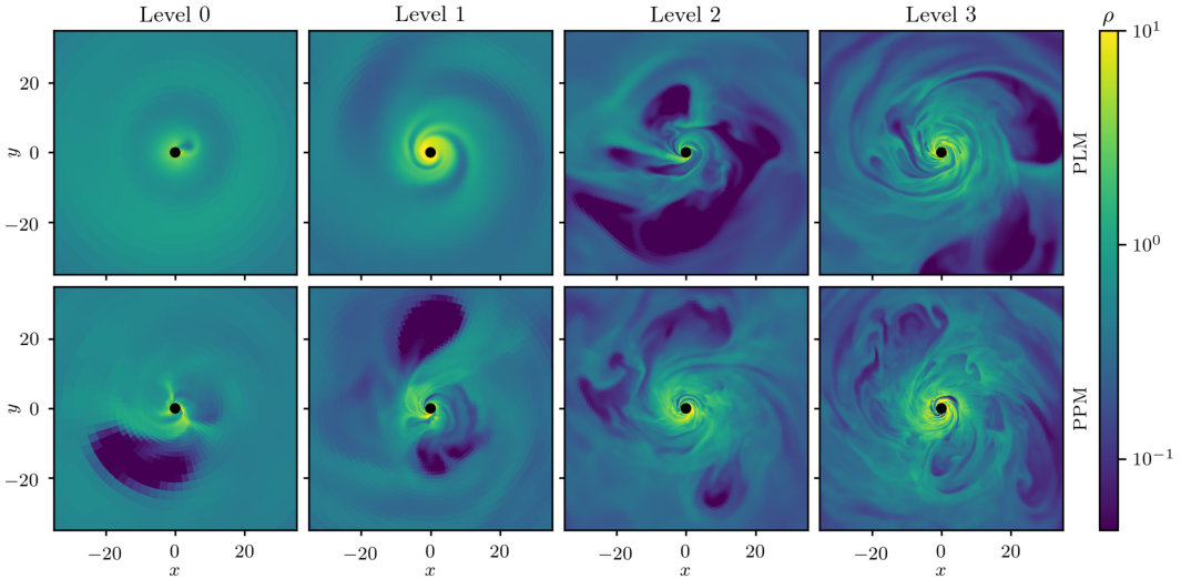 Figure 15
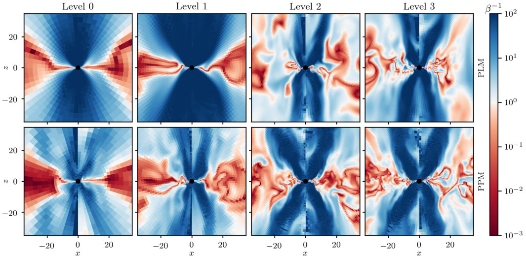 Figure 16
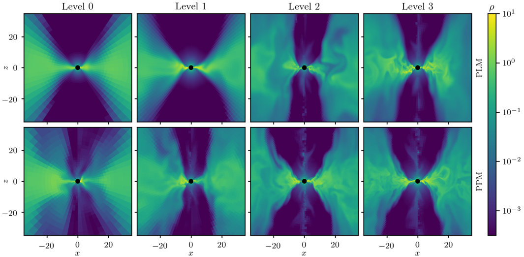 Figure 17
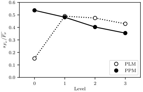 Figure 18
| Level | -rangeaaEvaluated at the midplane. Range may be less at higher latitudes. | bbNumber of cells needed to extend resolution within range to entire domain. | cells/decade | -rangeccEvaluated at small radii. Range may differ at large radii. | bbNumber of cells needed to extend resolution within range to entire domain. | |
|---|---|---|---|---|---|---|
| 0 | 1.078–1000 | 64 | 22 | 0–π | 32 | 64 |
| 1 | 1.078–1000 | 128 | 43 | π/8–7π/8 | 64 | 128 |
| 2 | 1.078–1000 | 256 | 86 | 3π/16–13π/16 | 128 | 256 |
| 3 | 1.078–.118.2 | 512 | 173 | 3π/8–5π/8 | 256 | 512 |
| Run | (%) | ||||||||||||||
|---|---|---|---|---|---|---|---|---|---|---|---|---|---|---|---|
| PLM–0 | 8\@alignment@align.39 | 0.59 | 51\@alignment@align.2 | 1.0 | 0\@alignment@align.190 | 0.029 | 1\@alignment@align.76 | 0.60 | 103\@alignment@align.1 | 2.5 | 0\@alignment@align.1513 | 0.0048 | |||
| PLM–1 | 12\@alignment@align.8 | 3.8 | 53\@alignment@align.2 | 7.1 | 0\@alignment@align.69 | 0.18 | 1\@alignment@align.243 | 0.034 | 118\@alignment@align | 29 | 0\@alignment@align.490 | 0.016 | |||
| PLM–2 | 15\@alignment@align.7 | 6.2 | 51\@alignment@align.1 | 8.0 | 0\@alignment@align.47 | 0.47 | 0\@alignment@align.788 | 0.026 | 107\@alignment@align | 36 | 0\@alignment@align.475 | 0.015 | |||
| PLM–3 | 15\@alignment@align.8 | 7.2 | 52\@alignment@align.7 | 8.8 | 0\@alignment@align.37 | 0.34 | 0\@alignment@align.545 | 0.027 | 133\@alignment@align | 48 | 0\@alignment@align.429 | 0.014 | |||
| PPM–0 | 13\@alignment@align.5 | 4.3 | 40\@alignment@align.9 | 8.8 | 0\@alignment@align.96 | 0.34 | 1\@alignment@align.360 | 0.060 | 100\@alignment@align | 37 | 0\@alignment@align.537 | 0.017 | |||
| PPM–1 | 14\@alignment@align.9 | 6.0 | 52\@alignment@align.1 | 8.6 | 0\@alignment@align.56 | 0.57 | 0\@alignment@align.834 | 0.014 | 141\@alignment@align | 43 | 0\@alignment@align.482 | 0.015 | |||
| PPM–2 | 16\@alignment@align.3 | 6.7 | 57\@alignment@align.3 | 7.6 | 0\@alignment@align.47 | 0.47 | 0\@alignment@align.575 | 0.023 | 153\@alignment@align | 51 | 0\@alignment@align.403 | 0.013 | |||
| PPM–3 | 15\@alignment@align.6 | 6.5 | 56\@alignment@align.4 | 7.5 | 0\@alignment@align.37 | 0.33 | 0\@alignment@align.480 | 0.027 | 147\@alignment@align | 52 | 0\@alignment@align.355 | 0.011 | |||
Peer Reviews
No public reviews on file for this paper yet. If you reviewed it on a platform where reviews are public (OpenReview, ICLR, NeurIPS, ICML), you can paste yours below so the community can read it here.
Videos
No videos yet. Explain this paper in a talk, walkthrough, or lecture? Add one.
A Resolution Study of Magnetically Arrested Disks
Christopher J. White11affiliation: Kavli Institute for Theoretical Physics, University of California Santa Barbara, Kohn Hall, Santa Barbara, CA 93107, USA , James M. Stone22affiliation: Department of Astrophysical Sciences, Princeton University, 4 Ivy Lane, Princeton, NJ 08544, USA , and Eliot Quataert33affiliation: Department of Astronomy, University of California Berkeley, 501 Campbell Hall, Berkeley, CA 94720, USA
Abstract
We investigate numerical convergence in simulations of magnetically arrested disks around spinning black holes. Using the general-relativistic magnetohydrodynamics code Athena++, we study the same system at four resolutions (up to an effective cells) and with two different spatial reconstruction algorithms. The accretion rate and general large-scale structure of the flow agree across the simulations. This includes the amount of magnetic flux accumulated in the saturated state and the ensuing suppression of the magnetorotational instability from the strong field. The energy of the jet and the efficiency with which spin energy is extracted via the Blandford–Znajek process also show convergence. However the spatial structure of the jet shows variation across the set of grids employed, as do the Lorentz factors. Small-scale features of the turbulence, as measured by correlation lengths, are not fully converged. Despite convergence of a number of aspects of the flow, modeling of synchrotron emission shows that variability is not converged and decreases with increasing resolution even at our highest resolutions.
accretion disks, black hole physics, magnetohydrodynamics, relativistic processes
††software: Athena++ (White et al., 2016), ibothros
1 Introduction
The notion that accumulation of ordered magnetic field could qualitatively change the nature of an accretion flow was first investigated by Bisnovatyi-Kogan & Ruzmaikin (1974). Numerical simulations by Narayan et al. (2003) confirmed that poloidal flux could lead to an efficient conversion of gravitational energy into mechanical energy, even around a non-spinning black hole. These simulations showed a magnetically arrested disk (MAD), in which accretion was hampered by a strong magnetic barrier.
Simulations around spinning black holes followed (Hawley & De Villiers, 2004; Tchekhovskoy et al., 2011; McKinney et al., 2012), adding in some cases optically thin cooling (Avara et al., 2016) or radiative transfer (McKinney et al., 2015; Morales Teixeira et al., 2018). In some of these simulations, the outflowing energy was found to exceed the amount infalling. This can be attributed to the Blandford–Znajek process (Blandford & Znajek, 1977) at play, electromagnetically extracting energy from the spin of the black hole and using it to launch a jet. At the same time, magnetic field threading a disk is expected to launch a wind via the Blandford–Payne process (Blandford & Payne, 1982).
McKinney et al. (2012) ran a number of models in which they varied physical parameters such as black hole spin and magnetic field geometry to explore the MAD parameter space. Here we address the orthogonal issue of to what extent numerical results depend on numerical parameters. That is, how well do simulations of this nature capture all the relevant physics? In particular, four concerns we seek to address are:
In axisymmetry, MAD leads to a completely arrested inflow that is broken by occasional bursts of accretion, while fully 3D simulations show interchanges of dense, less-magnetized fluid with magnetically buoyant bubbles (Igumenshchev, 2008). The dynamics of a heavier fluid supported against gravity by a lighter fluid lend themselves to the magnetic Rayleigh–Taylor instability (RTI Kruskal & Schwarzschild, 1954), only recently studied analytically in this context (Contopoulos et al., 2016). Without sufficient resolution, one might not fully capture this nonaxisymmetric instability, and this can in turn affect the reported accretion of matter and magnetic flux. 2. 2.
One defining characteristic of the MAD state is suppression of the magnetorotational instability (MRI, Balbus & Hawley, 1991). However, merely knowing that the MRI is suppressed is not sufficient to determine the strength of turbulence in these flows, as mechanisms such as the aforementioned RTI can also induce turbulence, as for instance is found by Marshall et al. (2018). What resolutions sufficiently resolve turbulence? 3. 3.
However much or little the statistical nature of a turbulent disk may change with resolution, how much does this affect the smoother, highly magnetized, relativistic jet? Jets are an extremely important consequence of MAD conditions, especially given their observability. What resolutions are needed to be confident in simulations’ measured jet properties? 4. 4.
What impact does grid resolution have on directly observable quantities?
In order to address these concerns, we run a single MAD scenario around a rotating black hole, varying the resolution but not the physical parameters. We go up to an effective resolution of cells per decade in radius, cells in polar angle, and cells in azimuthal angle. Our simulations are performed with the GRMHD capabilities of Athena++ (White et al., 2016), which utilizes staggered-mesh constrained transport and transmissive rather than reflecting polar axis boundary conditions. We employ the HLLE Riemann solver (Einfeldt, 1988) commonly used in the GRMHD community. While this solver is not the least diffusive available, we have found that having even less diffusion adversely affects the robustness of these highly magnetized simulations around rapidly spinning black holes. The code can use either a piecewise linear method (PLM, van Leer, 1974) or the piecewise parabolic method (PPM, Colella & Woodward, 1984) for spatial reconstruction. In multiple dimensions both methods formally converge at second order in spatial resolution, though the latter often has significantly smaller errors. We run simulations with both methods, since the effect of using PPM over PLM is to better capture spatial variability, just as would occur with increasing resolution.
In §2 we provide details about the setup and running of the simulations. We then investigate the effect of resolution on the disk itself (§3), on the jetted outflow (§4), and on observable electromagnetic signatures (§5). Discussion and conclusions follow in §6 and §7.
2 Simulations
All of our simulations are done in the same spherical Kerr-Schild coordinates as defined in Gammie et al. (2003), where we will drop , , and the black hole mass from all expressions. The coordinates are regular at the outer horizon and have determinant given by . We set the spin to be . In some cases we will express quantities in the cylindrical version of these coordinates, obtained with the standard spherical-to-cylindrical transformations. That is, we have , where and . The metric determinant in these coordinates is given by . In what follows we will denote fluid-frame rest-mass density by ; fluid-frame gas pressure by ; -velocity components by ; normal-frame Lorentz factor by ; fluid-frame magnetic pressure by , where and is the electromagnetic field tensor; magnetic field components by ; and the plasma magnetization parameters by and .
We begin with a torus of material in hydrodynamical equilibrium, following the prescription of Fishbone & Moncrief (1976). We set the inner edge of the disk to be at , with the pressure maximum at . The fluid has a fixed adiabatic index . This value is chosen as a compromise between relativistically hot () electrons and relativistically cold () ions, as is done for example by Ryan et al. (2018) when more carefully considering the two-temperature nature of the accreting plasma. We add an initial magnetic field similar to that of Tchekhovskoy et al. (2011). That is, the initial field is purely poloidal, circulating about a point well outside the pressure maximum. Specifically, we take the vector potential to have only an azimuthal component
[TABLE]
where is the linear ramp function
[TABLE]
The field is normalized to have the density-weighted average of of the torus be .
Our root grid (refinement level 0) has cells in , , and . In radius it extends from to with logarithmic spacing, with the innermost cell entirely inside the horizon. The grid is uniform in and . We then add successive layers of static mesh refinement to the domain as follows. Each additional level refines all cells in its domain by a factor of in each dimension. Level 1 refinement covers at all radii and all polar angles for . Level 2 covers at all radii, for , and all polar angles for . Level 3 covers for . The grid is illustrated in Figure 1, where the grid lines are drawn every cells in and every cells in .
With this grid, the timestep at all refinement levels is limited by the -width of the (never-refined) cells at the base of the polar axis. The root grid has a radial resolution of approximately cells per decade, and each successive refinement level doubles this, up to cells per decade at the highest resolution. At the highest resolution there are cells in azimuth, and the polar resolution in the bulk of the disk is the same as an effective equally spaced cells. These values are detailed in Table 1.
\floattable
For comparison, the grid employed in Tchekhovskoy et al. (2011) and in model A0.99N100 of McKinney et al. (2012) (the only one with a spin approximately the same as ours) has cells in polar angle, cells in azimuth (doubled to midway through the simulation) and fewer than cells per decade in radius. The high-resolution runs A0.94BfN40, A-0.94BfN40HR, and A0.94BtN10HR of McKinney et al. all have cells per radial decade in the inner regions, effective polar cells based on the midplane resolution at , and cells in azimuth. A more recent study on MAD accretion, Avara et al. (2016), has an effective resolution of approximately cells in (used to resolve a thin disk) and cells in , while the tilted jets in Liska et al. (2018) are simulated with effective resolutions up to in angle. Except for this last case, our highest resolution typically has or more times as many total cells per dimension as these previous calculations.
We define the radial width of a cell to be the integral of over the line of constant and passing through the cell midpoint from one constant- face to another, and likewise for polar and azimuthal widths. (These reduce to the expected , , and in the Newtonian limit.) Then in the midplane our grid has varying from approximately at the inner boundary to at the outer boundary, while varies from to . Having aspect ratios near unity across all our grids is important, as refining only one or two dimensions will have little effect on reducing errors once those errors become dominated by the coarser dimensions.
A number of limits are imposed on the variables for numerical stability. The density and gas pressure are kept above the floors
[TABLE]
In addition, we enforce , , and . Whenever these limits are imposed, the magnetic field is left unaltered. For comparison, Tchekhovskoy et al. (2011) enforce either and or else and (stating that the choice makes little difference), while McKinney et al. (2012) have and . More recent work by Liska et al. (2018), which includes strong fields launching jets, uses the limits and , while also enforcing and .
We start with a single simulation with level 3 refinement and PPM reconstruction, running until time . This checkpoint is then coarsened to the other grids, and all simulations are then run from to , using both PLM and PPM. When averaging results in time, we choose in all cases.
To run for a simulation time of , the level 3 PPM simulation took node-hours on Intel Knights Landing (Xeon Phi 7250) nodes, with cores per node. The level 2 PPM simulation took node-hours on Intel Skylake (Xeon Platinum 8160) nodes, with cores per node.
3 Disk Properties
3.1 Mass Accretion Rate
We define the mass accretion rate at a fixed time through a sphere of fixed radius to be
[TABLE]
Positive values correspond to inflow. Figure 2 shows the run of with , averaged in time, for our simulations. In steady state, we expect to be independent of radius, and indeed we do see an extended plateau. There is a small rise inward at very small radii (). This is an artifact of numerical floors, and it measures the small amount of mass added by the floors at these radii. Other simulations using different codes see the same effect; see for example Figure 4 of Morales Teixeira et al. (2018). The four level 2 and level 3 simulations agree on the plateau height. At sufficiently low resolutions, the accretion rate is underestimated. Moreover, there is a cell-to-cell oscillatory numerical artifact that occurs at very low resolutions when using PPM, almost certainly due to the slope limiter itself. There is no sign of this effect at higher resolutions.
When fixing a single radius at which to measure , we choose from here on. Using this radius, we show the values of as a function of time in Figure 3. In all cases except the lowest-resolution PLM simulation, the accretion becomes highly variable, experiencing order-unity changes even on the timescale of between snapshots. In order to make the figure clearer, we smooth the accretion rate with a Gaussian filter of full-width at half-maximum . (This smoothing accounts for the lines differing at , when all the simulations are identical.) The average accretion rates are not changing significantly over time, and there are many oscillations in the time window from to , justifying our time averages. We note that recent work by Balbus (2017) suggests unstable modes near the innermost stable circular orbit (ISCO) can disrupt the inner parts of disks, suggesting caution when searching for and interpreting steady-state values of .
3.2 Accumulation of Magnetic Flux
The MAD state is characterized by strong poloidal magnetic flux, which we can measure in a number of ways. Following Tchekhovskoy et al. (2011) and McKinney et al. (2012) we can integrate radial flux through spheres of different radii to define
[TABLE]
Our explicit factor of is implicit in the units in Tchekhovskoy et al. (2011). We can also define the midplane vertical flux out to a radius by either of two equivalent formulas:
[TABLE]
counts only flux that passes through the midplane, while also includes field lines that terminate at the horizon. Figure 4 shows both measures of flux, time-averaged, as a function of radius. As for the inner part of the disk, most of the magnetic field lines here terminate at the horizon. These profiles agree in the region where steady-state accretion has been attained. Thus even at low resolution we are capturing the large-scale structure of the magnetic field.
As in Tchekhovskoy et al. (2011), we normalize the horizon flux based on each simulation’s average accretion rate. We choose to use the difference , as the value of this quantity at any radius is the flux on the horizon so long as the field is essentially vertical (all field lines are either outside the sphere and midplane annulus, cross the sphere twice and the midplane once, or cross the sphere once and terminate on the horizon). We define
[TABLE]
Here the fluxes and accretion rate are evaluated at . The time-averaging is done with a Gaussian filter of full-width at half-maximum . Figure 5 shows the results. The average level and variability in for most of our cases is similar to that found by Tchekhovskoy et al. (2011), where the saturated state has . (Note there exists another common flux normalization, denoted , that is approximately a factor of times smaller than at the horizon for our spin.) At the lowest resolution, PPM can still capture some of the variability, though the accumulated flux is too low. At that resolution, PLM gives no time variability, again indicating the numerics in that case are not sufficiently capturing the turbulent nature of the flow.
3.3 The Magnetorotational Instability
The crucial qualitative difference between a true MAD state and a disk with just a strong field is the inhibition of the MRI due to the field. In order to investigate if this has indeed occurred, we compare the marginally stable wavelength for the vertical MRI to the disk scale height.
The general-relativistic dispersion relation relating Alfvén frequency to oscillation frequency for a mode is given by Gammie (2004):
[TABLE]
Here is the epicyclic frequency and we have
[TABLE]
The dispersion relation is quadratic in , and the critical frequency corresponds to the value of such that the lesser quadratic root for vanishes. This is simply , as can be easily verified. Now is a frequency as measured by a local observer on a circular orbit. Gammie gives the prescription for transforming this into a frequency as seen by an observer at infinity. The result is the instability criterion
[TABLE]
where
[TABLE]
is the relativistic correction to the standard formula (cf. the nonrelativistic version \tagform@108 from Balbus & Hawley, 1998). This correction necessarily approaches unity as ; it also diverges as , meaning the effect of general relativity is to stabilize the inner disk. Note some sources omit the in their definition of .
For the scale height, we adopt a definition similar to that found in McKinney et al. (2012), though we vary vertical coordinate rather than polar coordinate . That is, for given , , and , we calculate
[TABLE]
where the cutoffs are chosen to be . Then the scale height at that location is given by
[TABLE]
Figure 6 shows the radial profiles of and , each averaged in and . Also shown is the height of a single cell at the midplane. Except at the innermost few gravitational radii, reaches or exceeds the scale height throughout the inner regions of all the disks, indicating these are sufficiently MAD to inhibit the MRI. Disk scale height is relatively invariant across simulations, as is the run of in the regions that have reached steady state. At the lowest resolutions we are only marginally resolving and , though at higher resolutions we have many cells per critical wavelength and per scale height.
We define an MRI suppression factor . This counts the number of critical wavelengths spanning the full disk, so the instability is expected to be unimportant for . Note the suppression factor in McKinney et al. (2012) differs from ours by a factor of , and so their cutoff of corresponds to with our definition. The fact that is small even in the lowest resolutions, where we have already seen other evidence of underresolved behavior, indicates that building up enough vertical flux to suppress the MRI is only a matter of physical conditions and that any reasonable resolution is numerically capable of showing the effect.
Gammie (2004) also gives formulas corresponding to the maximum growth rate. This occurs at a wavelength of
[TABLE]
where again we have a relativistic correction factor
[TABLE]
multiplying the Newtonian version (\tagform@114 in Balbus & Hawley, 1998). From this we can define a vertical MRI quality factor counting the number of cells in a single wavelength of the fastest growing mode:
[TABLE]
Taking an -weighted mean of at the midplane inside , we find that the PLM simulations have average quality factors of , , , and , and the PPM simulations have values of , , , and . The lower two resolutions are only marginally resolving the MRI according to Hawley et al. (2011).
3.4 Disk Structure
Late-time snapshots of the midplane density structures of the disks for all our runs is shown in Figure 7. At the lowest resolutions little azimuthal variation is present. The remaining simulations show low-density magnetically supported bubbles repeatedly forming and rising buoyantly away from the black hole, as we expect from the magnetic RTI. These bubbles are well resolved where they appear, with their sizes being roughly independent of the grid scale. Still there is a clear trend of increasingly finer structure appearing at higher resolutions, with secondary instabilities appearing at the surfaces of the bubbles in the higher-resolution PPM simulations.
Figure 8 shows plasma in the same midplane slices. Dark red lines indicate field reversals and thus current sheets. They become thinner and more numerous at higher resolution and also at fixed resolution when transitioning from PLM to PPM.
We also show late-time vertical slices through the simulation, colored by (Figure 9) and (Figure 10). In both cases there is structure down to the grid scale, with current sheets generally being a single cell thick.
The amount of structure can be more quantitatively expressed via correlation lengths of various quantities. We do this with correlations in the azimuthal direction in the midplane, following Shiokawa et al. (2012). We define the time-dependent correlation function for a quantity to be
[TABLE]
where is the change in a quantity from its mean over the same domain, the range covers a single cell in radius, and the range covers the two cells in polar angle bordering the midplane. We normalize and average this to obtain the time-independent correlation function
[TABLE]
Figure 11 shows the run of the time-independent correlation function with at representative value of , calculated for . While large-scale features may be captured almost as well by the level 1 simulations as those at level 3, correlations at small scales are still changing with resolution between levels 2 and 3.
The essence of our correlation functions can be summarized by a single correlation length at each radius. The correlation length at a given radius is the value for which . Note that these lengths are in fact angles.
The correlation lengths for and are shown in Figure 12. In all cases the angular length scales are invariant with radius over the inner region in which steady state has been achieved. At some fixed resolutions, correlation lengths in the plateau region are slightly lower when using PPM as opposed to PLM, and also slightly lower when looking at rather than , but these differences are small compared to the effect of resolution. We have not achieved convergence, though the values we measure suggest convergence might be achieved with approximately two more levels of refinement (a factor in resolution).
It is interesting to note that the correlation lengths shown in Figure 12 are much larger than the azimuthal cell widths, which range from to . This is partly expected from having small structures sheared out in the azimuthal direction: the direction in which we measure correlations is not orthogonal to the current sheets. Furthermore, as noted in White et al. (2016) when comparing such correlations in non-MAD disks to those found by Shiokawa et al. (2012), at fixed -resolution midplane correlation lengths can decrease with increasing -resolution in the midplane. That is, one should use caution in comparing these correlation lengths between simulations with different polar grids. We expect then that had we concentrated our grid near the midplane these particular correlation lengths would have been lower.
As there is no explicit dissipation mechanism in these simulations, it is expected that some turbulent properties continue to scale with the grid size and corresponding magnitude of numerical dissipation. However the non-convergence of small-scale turbulence does not necessarily preclude the convergence of global properties, especially in MAD flows. In contrast to cases with no net vertical flux, the transport of angular momentum in these flows can be dominated by large-scale magnetic stresses instead of stresses resulting from small-scale turbulence. This explains how our accretion rates can agree at sufficiently high resolution even when our correlation lengths do not.
4 Jet Properties
4.1 Magnetic Structure
While most of our simulations are quite turbulent, they do reach steady state in the average sense and so regions can be defined based on their - and -averaged properties. We do this with two measures of magnetization, plasma and . Figure 13 shows the results for the level 3 PPM run (the other runs appear similar). As suggested in McKinney et al. (2012), we can loosely define the disk to be where gas pressure dominates magnetic pressure, the jet to be where magnetic energy density dominates rest mass energy density, and the corona to be the region in between. The colorschemes in the figure emphasize these transitions at and .
In order to compare our simulations, we sample average magnetization along arcs of constant and varying . The results are shown in Figure 14. The results across the simulations are in generally good agreement, with two exceptions. First, the lowest resolutions show slightly less magnetization in the bulk volume of the jet, outside the core. Second, there is a trend of disk magnetization increasing with resolution. While even very low resolutions can capture the qualitative structure of the magnetized accretion flow (agreeing with the findings in §3.2), the quantitative amount of magnetization relative to the hydrodynamical state of the disk is another example of a property that has not entirely converged.
While and are large near the poles, they are below the numerical ceilings of at the sampled radius. We caution however that the magnetization could be larger closer to the horizon. Once the jet has propagated some distance it is no longer affected by the ceilings, but they could leave an imprint by adding density and pressure at very small radii.
4.2 Energy Extraction
Just as with mass, we can calculate the flux of covariant (binding) energy through a spherical surface:
[TABLE]
The efficiency of the black hole is taken to be
[TABLE]
where the denominator is smoothed in time with a Gaussian filter of full-width at half-maximum . Given that always (cf. Figure 3), corresponds to some positive energy (negative binding energy) being transported to infinity. If this is simply the binding energy of a circular orbit at the ISCO relative to [math] at infinity, as in the Novikov–Thorne model, we expect for . In cases where , this energy exceeds not only the binding energy but also the rest-mass energy of the matter falling into the black hole, and we expect to see this given high spin and a MAD disk (Tchekhovskoy et al., 2011).
Figure 15 shows the energy extraction and efficiency as functions of time. As with other quantities that reflect the turbulent nature of these flows, the time series are highly variable, though again the level 0 PLM run shows no significant variability. At higher resolutions and with higher-order reconstruction, the energies and efficiencies are slightly higher, though the differences are somewhat obscured by the high variability.
Most of the measured efficiencies exceed unity, going up to approximately . Even the level 0 PLM run shows , whereas we would expect if the accretion flow were not in the MAD state, or if the black hole were not spinning.
We can differentiate between energy in the jet and energy in the wind by labeling locations as one of “jet,” “wind,” or “disk” according to the average accretion state as pictured in Figure 13. Constructing these averages for all eight simulations, we define the jet to be where , the wind to be where and , and the disk to be the remaining volume. The disk contributes negligibly (less than ) in all cases to the energy flux used to calculate . Among the PLM simulations, the jet comprises , , , and of the energy flux in order of increasing resolution. For PPM, these values are , , , and .
The jet contributions to alone are far larger than the Novikov–Thorne efficiency. Thus the Blandford–Znajek mechanism for extracting spin energy from the black hole is robustly modeled, even at moderate resolutions that do not fully capture other aspects of the accretion flow.
4.3 Jet Structure
While the rate of spin energy extraction may not vary much with resolution, the jet structure can change. Figure 16 shows cylindrical radial profiles of fluxes in the jet in the planes (averaging the results for the two planes). In particular, we plot the outward mass flux per unit area and outward binding energy per unit area . This later quantity is negative where energy is flowing to infinity. Total fluxes through the planes correspond to integrating the values against .
In these planes, the jet () is inside , as can be seen in Figure 14. Immediately outside the jet there is considerable coronal outflow of mass in all simulations. Inside the jet region, the mass flux becomes negligible, with a large amount of energy flowing outward in the form of Poynting flux.
Our refinement scheme refines the jet in these planes, though the jet base is always on a coarse grid. Any resolution-dependent effects we see are therefore due to processes in the jet but beyond the base, or else due to properties of the disk. In fact there is very little variation in jet flux profiles with disk resolution. However, all PPM simulations consistently concentrate much of the energy flux in a narrow jet core, while the PLM simulations have a much broader distribution in . This suggests the jet structure would change if the resolution of the always-coarse jet base were altered, likely appearing more like the PPM results at higher resolution.
Figure 17 shows the Lorentz factor of the fluid, relative to the normal observer, through these same planes. Here the effects of resolution are more noticeable. The similarity of the level 2 and level 3 PPM profiles might indicate convergence, though the grid resolution in the jet region does not change between these two refinement schemes. Qualitatively, all runs show similar off-axis peaks in Lorentz factor, with the core being slower than the jet walls.
We caution that properties of this highly magnetized, rapidly moving part of the flow can depend numerically on not only resolution, but also the treatment of floors and variable inversion failures. Radial profiles of mass and internal energy fluxes indicate that density and gas pressure floors add only very small amounts of material and heat in our simulations. Still, the ideal MHD condition means that even with perfect magnetic field evolution, electric fields and thus electromagnetic energies are sensitive to any changes in fluid velocity resulting from numerical floors.
5 Light Curves
The results of the previous sections show some of the physical properties of the accretion flow are converged with resolution while others are not. This raises the question of how converged are direct observables. While our simulations do not model photons in situ, we can postprocess snapshots in order to generate light curves from the simulations. For this purpose we choose to use the code ibothros, which models synchrotron emission and absorption and propagates photons along geodesics in the Kerr spacetime to generate an image of specific intensity at a given frequency.
We must set several physical scales, and we choose these to reflect the supermassive black hole in M87. Following Ryan et al. (2018) we set the black hole mass to , placed at a distance of . We choose a viewing angle off the jet axis. The electron density is taken to trace the fluid density, with a constant temperature ratio of between the ion and electron temperatures, and the electrons are assumed to be thermal. Images are sampled every (i.e. every days) over the simulations times (i.e. spanning years). Each image consists of pixels covering a patch of sky () on each side. The density scale of the fluid is adjusted until the total emission at matches the observed value of from Doeleman et al. (2012).
Except in the level 0 PLM case, where the flux varies monotonically with time, the light curves all display variability about a saturated state. The standard deviations of the fluxes are shown in Figure 18. The standard deviations of these standard deviations are small, less than in all cases, making the trend with resolution statistically significant. That is, variability is decreasing with increasing resolution, and it does not appear converged at our highest resolution.
6 Discussion
In examining the same problem of MAD accretion at different resolutions, we can determine which properties have converged and are therefore the most robustly determined by simulations.
The large-scale structure of the accretion flow is relatively constant across our simulations. In particular, the time-averaged magnetization as depicted in Figure 13 roughly holds at all resolutions. This is reflected in the constancy of where the solid lines cross the dotted lines in the lower panels of Figure 14, as well as the similar sizes of magnetic bubbles shown in Figures 7 and 8.
Figure 6 shows that the MRI is robustly suppressed in the inner part of all our simulations. Even at low resolutions, we can see that the critical wavelength of the MRI tracks the disk scale height. Our initial setup thus robustly leads to a MAD state in the sense of growth of the MRI being suppressed by buildup of magnetic flux and compression of the disk. This occurs even at lower resolutions where the MRI quality factors indicate we are only moderately sampling unstable wavelengths.
A number of important global parameters converge at sufficiently high resolution, including the accretion rate (Figures 2 and 3), the vertical magnetic flux near the horizon (Figure 4 and 5), and the rate of energy extraction from the black hole (Figure 15). This last quantity is highly variable in time in the MAD state, and so longer run times would allow for a more precise measurement of the mean efficiency.
We consistently find about times as much outgoing energy in the magnetized jet as in the wind. This is in agreement with the values of and reported in Table 5 of McKinney et al. (2012) for comparable models (A0.9N25, A0.9N50, A0.9N100, A0.9N200, and A0.99N100). On the other hand, the MAD models of Avara et al. (2016) and Morales Teixeira et al. (2018) have more energy leaving through the wind than the jet. This can be an effect of the thinness of those radiatively cooled disks, as well as the fact that they only have , meaning the Blandford–Znajek process will produce a much weaker jet.
Other aspects of the flow show signs of converging, though there is disagreement at our highest resolutions, indicating somewhat higher resolutions are required to attain convergence. For example, the midplane values of magnetization as measured by agree at high resolutions, but there is still disagreement when using (Figure 14). The quantitative measure of MRI suppression, , follows in not being fully converged.
The statistical nature of the turbulence, as measured by correlation lengths, has also not quite converged (Figures 11 and 12); size scales decrease as resolution increases (and they decrease slightly as higher-order reconstruction is used). Figure 11 in particular is essentially a power spectrum and captures the same information as the azimuthal power spectra computed by Morales Teixeira et al. (2018), who see agreement among simulations that only have up to cells within . They have at most azimuthal cells per correlation length and see convergence while we have up to cells per correlation length ( cells with a length of ) and do not have the same agreement. This discrepancy is likely due to the radiative nature of their disks.
It may seem inconsistent that we easily suppress the MRI even at low resolutions and yet we do not attain convergence in turbulence at our highest resolution. This tension is resolved by having another driving force for turbulence, the magnetic RTI. Marshall et al. (2018) study the stresses in a thinner MAD disk, and they also see turbulent angular momentum transport despite MRI suppression, attributing this to the constant formation and disruption of Rayleigh–Taylor bubbles.
The jet Lorentz factor (Figure 17) is another quantity whose values may still change with higher resolution. It is somewhat surprising that energy extraction shows less discrepancy between different resolutions than Lorentz factor. We reiterate that the jet base has the same grid in all our simulations, so we can only measure convergence in terms of properties that depend on resolving disk properties and resolving the propagation of the jet tens of gravitational radii beyond the horizon.
Some properties are far from converged in our simulations. The thinnest current sheets are always at the grid scale (Figures 8 and 10), and secondary instabilities on top of Rayleigh–Taylor bubbles do not even appear except at the highest resolutions (Figure 7).
More disconcerting is the trend light curve variability has with resolution (Figure 18). We are possibly far from convergence, which one expects if the short-timescale variability comes from small, transient, highly magnetized parcels of plasma that are not well resolved on the grid.
We summarize key average quantities for the simulations in Table 2. For the accretion rate and horizon magnetic flux we take a simple average in time, quoting the standard deviation of the samples in the range . We do the same for the efficiency but with fewer samples, as times at the very end of time simulation cannot be used due to the width of the Gaussian filter used in calculating these quantities. For the MRI suppression factor , we average the scale height and critical wavelength in azimuth, calculate , and then average in time. Then and the density correlation length have been time averaged, but we must find a way to average in radius. For we define
[TABLE]
and
[TABLE]
where the integrals are over the region , using , , , and samples at levels 0 through 3. The table reports for all five of these measures. For the values of in each light curve, we define to be the unbiased estimator of the variance of the set, with the uncertainty in taken to be
[TABLE]
in terms of the gamma function. The table reports , where the mean used to normalize is always within of the observed .
\floattable
Of the quantities in the table, the horizon-penetrating flux is the most clearly converged, showing similar values even at the lowest resolutions. The accretion rate , MRI suppression factor , and efficiency also appear converged at the resolutions of refinement levels 2 and 3, though these are intrinsically highly variable statistics in these flows. Turbulent correlation length and synchrotron light curve variability do not converge by level 3.
7 Conclusion
We study a single physical scenario of MAD accretion onto a rapidly spinning black hole at various resolutions. This is done employing the static mesh refinement ability of Athena++, spanning a factor of in resolution in each dimension over the bulk of the disk. By only varying resolution and comparing results, we can determine which features of such simulations are adequately resolved and can therefore be trusted. A priori, it is not obvious how much sensitivity to resolution we should expect in MAD structure given inward field advection is competing with the complex nonlinear processes of turbulent diffusion and magnetic RTI.
Certain global properties are found to converge with resolution in our set of simulations, notably accretion rate and jet efficiency , as well as the fact that the MRI is suppressed. Magnetic structure is generally well captured. In particular, the accumulated magnetic flux on the horizon is found to be essentially the same at all resolutions we consider. Buoyant magnetic bubbles are well resolved on the higher resolution grids (though with secondary Kelvin–Helmholtz instabilities only appearing at high resolution with higher-order spatial reconstruction).
As simulations in the literature use grids that go up to our levels 2 and 3 (Tchekhovskoy et al., 2011; McKinney et al., 2012; Avara et al., 2016), going even higher in some cases (Liska et al., 2018), these results provide assurance that the large-scale structures of MAD flows are being accurately modeled by the community.
On the other hand, the details of jet structure, including profiles of energy flux and Lorentz factor, do not agree among our simulations. Higher resolutions at the base of the jet itself would be helpful in reliably determining the velocity and energy distributions between the core and outer parts of the jet. The Lorentz factor too will probably change at higher resolutions, though increasing resolution alone will very likely not be enough to create jets with given that in all our jets peaks between and .
We do not see convergence in the length scales of turbulent eddies, though these scales may converge with another factor of approximately in resolution. We also do not see convergence in the thicknesses of current sheets, and indeed this is not surprising given the lack of any explicit dissipation mechanism decoupled from the grid scale in the simulations.
The lack of convergence in small-scale features would not necessarily be a concern, except these features can affect observables. One might hope that in going from accretion flows with disordered magnetic fields to MAD flows, with small-scale turbulence giving way to large-scale magnetic stresses as the important transport mechanism, the emitted light will be less sensitive to the resolution. However, when postprocessing our simulations to model thermal synchrotron emission, we see that there is light curve variability that continues to scale with resolution even at the highest resolutions (Figure 18). There are certainly caveats to these findings — including not modeling the radiation dynamically, not including other radiative processes such as Compton scattering, and not considering nonthermal particles — indicating future avenues of exploration. Still, our results suggest caution in comparing simulations to data via light curves, even when most aspects of the simulation appear converged.
We conclude that the general MAD flow structure is robust. This includes the suppression of the MRI as well as the field structure that results from an equilibrium between inward advection and the rising of magnetically buoyant bubbles in a setting unstable to RTI. Details of turbulence are however not fully captured at these resolutions, in the sense that some observable quantities are affected by our choice of grid, and this can affect observables.
We relegate the computationally expensive study of resolution at the base of the jet to a separate investigation. Future simulations with in situ radiative transfer can help further determine to what extent the variation of turbulence with resolution has on direct observables.
We thank S. M. Ressler for help in using ibothros on our data. This work used the Extreme Science and Engineering Discovery Environment (XSEDE) Stampede2 at the Texas Advanced Computing Center through allocation AST170012, resources of the Argonne Leadership Computing Facility (ALCF) via the Innovative and Novel Computational Impact on Theory and Experiment (INCITE) program, and the Savio computational cluster resource provided by the Berkeley Research Computing program at the University of California, Berkeley. This work was supported in part by a Simons Investigator award from the Simons Foundation and NSF grants AST 13-33612 and AST 17-15054 (EQ).
The reference list from the paper itself. Each links out to its DOI / PubMed record.
- 1Avara et al. (2016) Avara, M. J., Mc Kinney, J. C., & Reynolds, C. S. 2016, Monthly Notices of the Royal Astronomical Society, 462, 636
- 2Balbus (2017) Balbus, S. A. 2017, Monthly Notices of the Royal Astronomical Society, 471, 4832
- 3Balbus & Hawley (1991) Balbus, S. A., & Hawley, J. F. 1991, The Astrophysical Journal, 376, 214
- 4Balbus & Hawley (1998) —. 1998, Reviews of Modern Physics, 70, 1
- 5Bisnovatyi-Kogan & Ruzmaikin (1974) Bisnovatyi-Kogan, G., & Ruzmaikin, A. 1974, Astrophysics and Space Science, 28, 45
- 6Blandford & Payne (1982) Blandford, R., & Payne, D. 1982, Monthly Notices of the Royal Astronomical Society, 199, 883
- 7Blandford & Znajek (1977) Blandford, R., & Znajek, R. 1977, Monthly Notices of the Royal Astronomical Society, 179, 433
- 8Colella & Woodward (1984) Colella, P., & Woodward, P. R. 1984, Journal of Computational Physics, 54, 174