TL;DR
This paper investigates a data assimilation method for large-Prandtl Rayleigh-Bénard convection using temperature observations, providing theoretical guarantees and numerical validation, with implications for geophysical and high-pressure gas applications.
Contribution
It introduces a rigorous framework for data assimilation in large-Prandtl convection, identifying conditions for synchronization and validating them through simulations.
Findings
Synchronization often occurs beyond theoretical conditions
Conditions are practically relevant only at extremely large Prandtl numbers
Numerical results confirm theoretical predictions
Abstract
This work applies a continuous data assimilation scheme---a particular framework for reconciling sparse and potentially noisy observations to a mathematical model---to Rayleigh-B\'enard convection at infinite or large Prandtl numbers using only the temperature field as observables. These Prandtl numbers are applicable to the earth's mantle and to gases under high pressure. We rigorously identify conditions that guarantee synchronization between the observed system and the model, then confirm the applicability of these results via numerical simulations. Our numerical experiments show that the analytically derived conditions for synchronization are far from sharp; that is, synchronization often occurs even when the conditions of our theorems are not met. We also develop estimates on the convergence of an infinite Prandtl model to a large (but finite) Prandtl number generated set of…
Click any figure to enlarge with its caption.
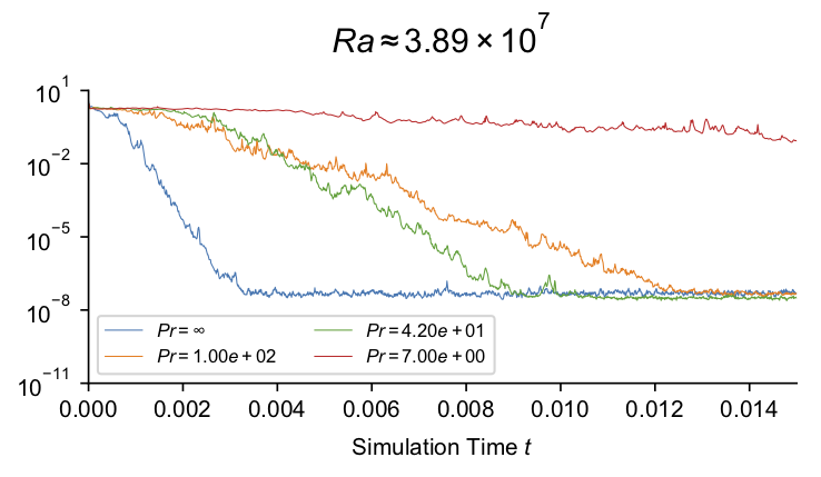 Figure 1
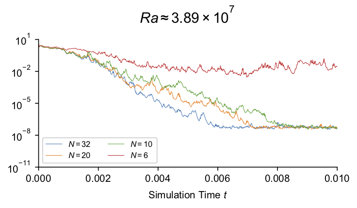 Figure 2
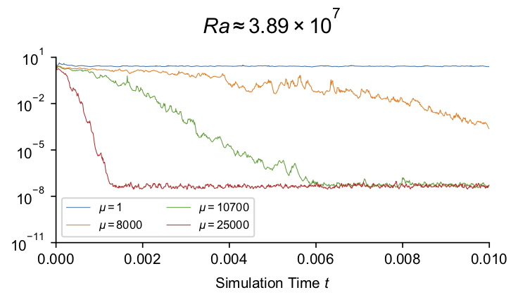 Figure 3
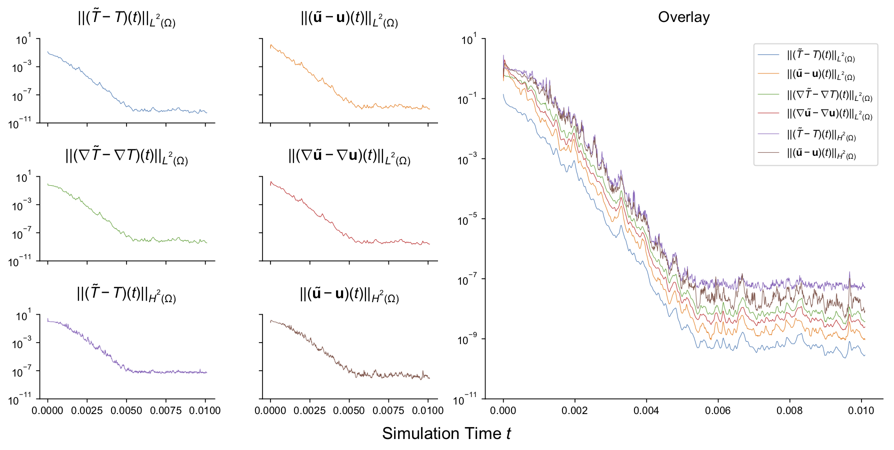 Figure 4
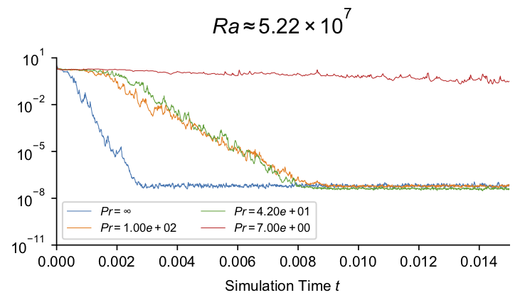 Figure 5
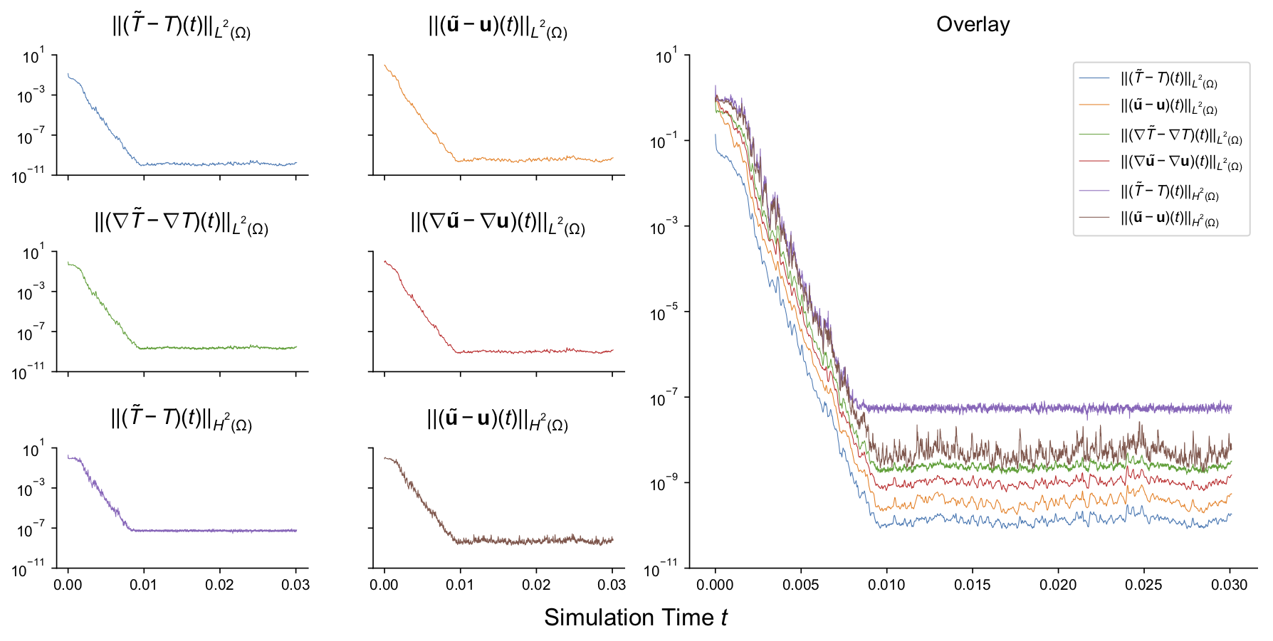 Figure 6
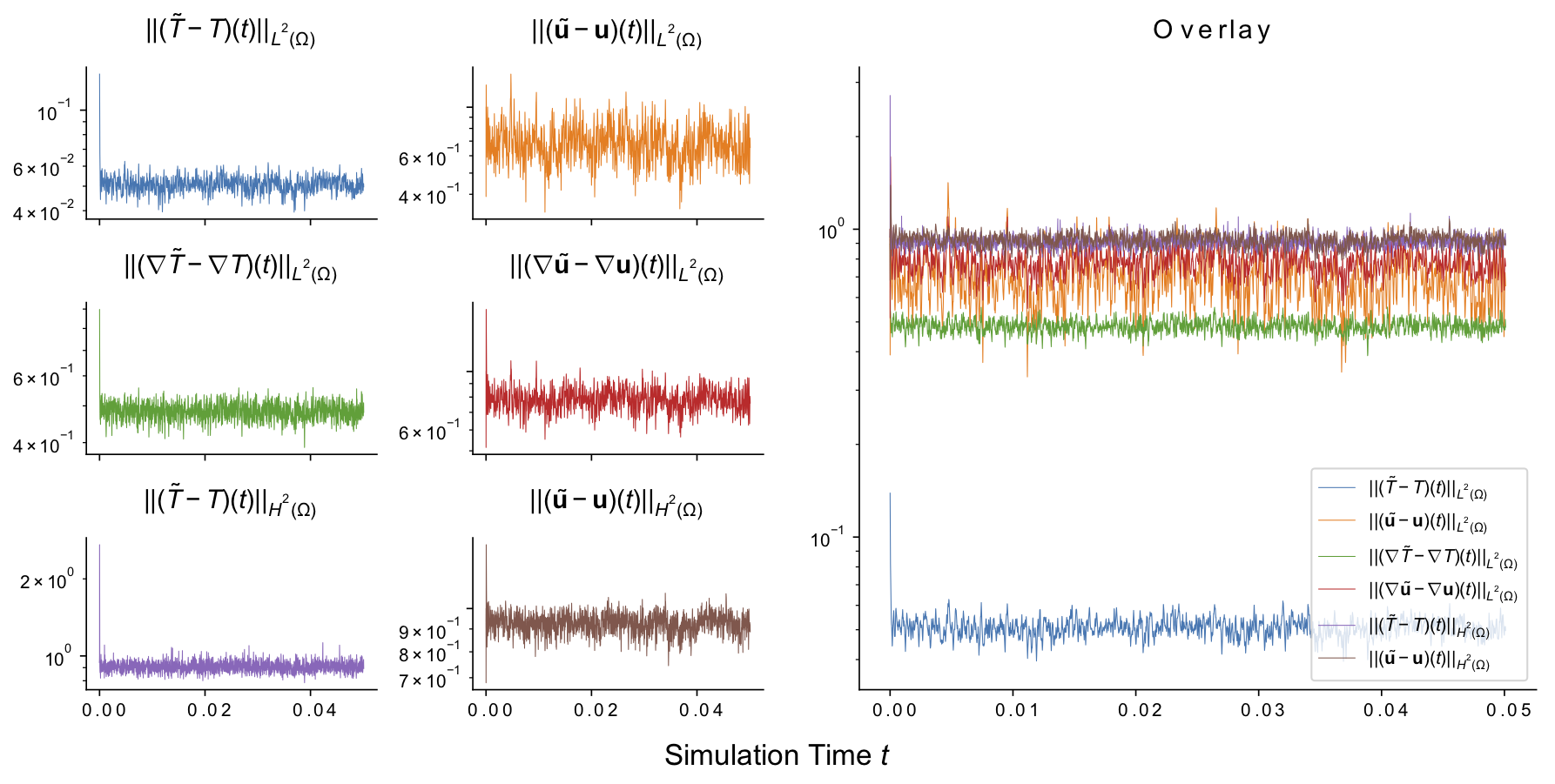 Figure 7
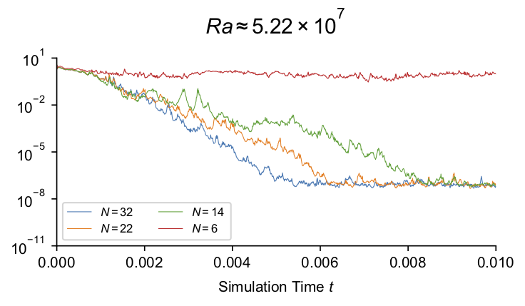 Figure 8
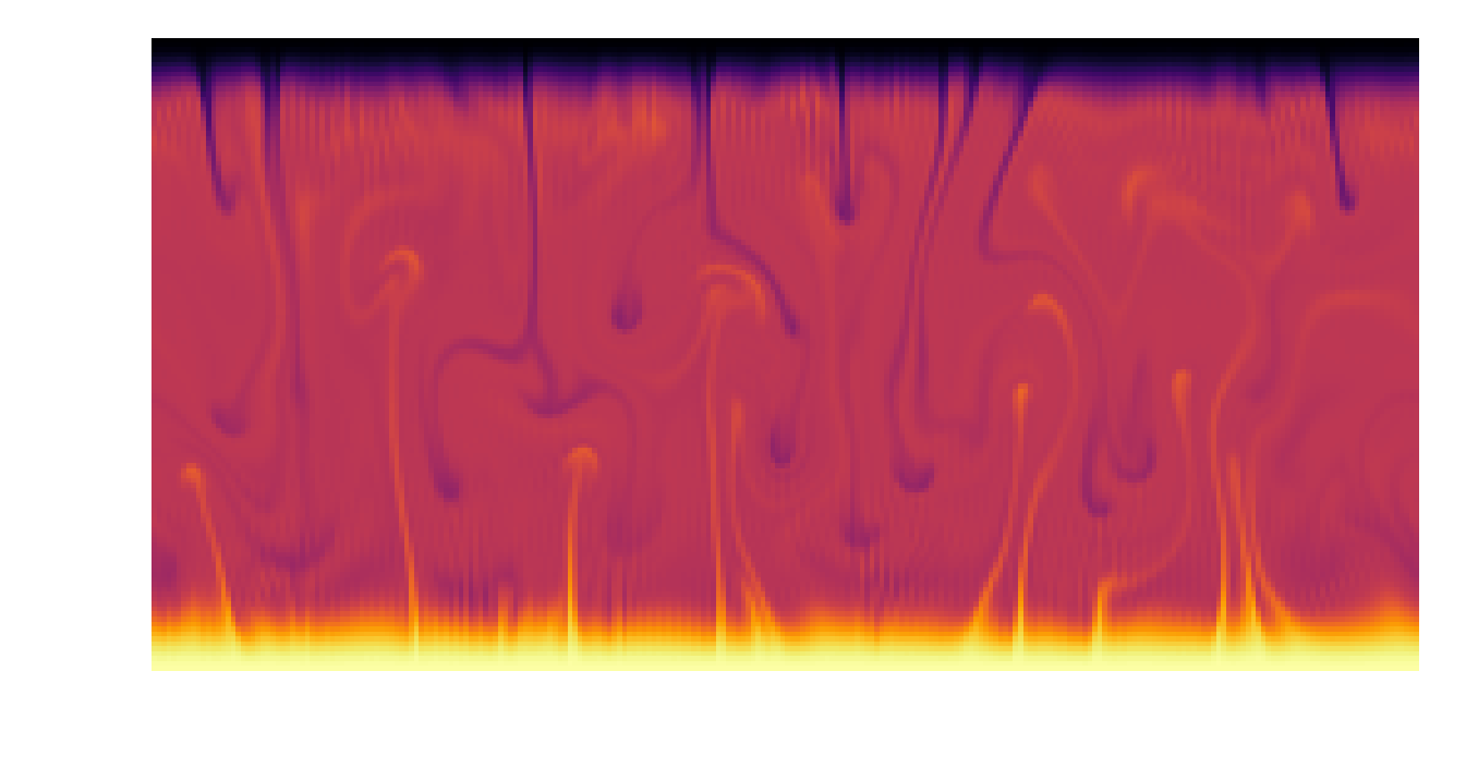 Figure 9
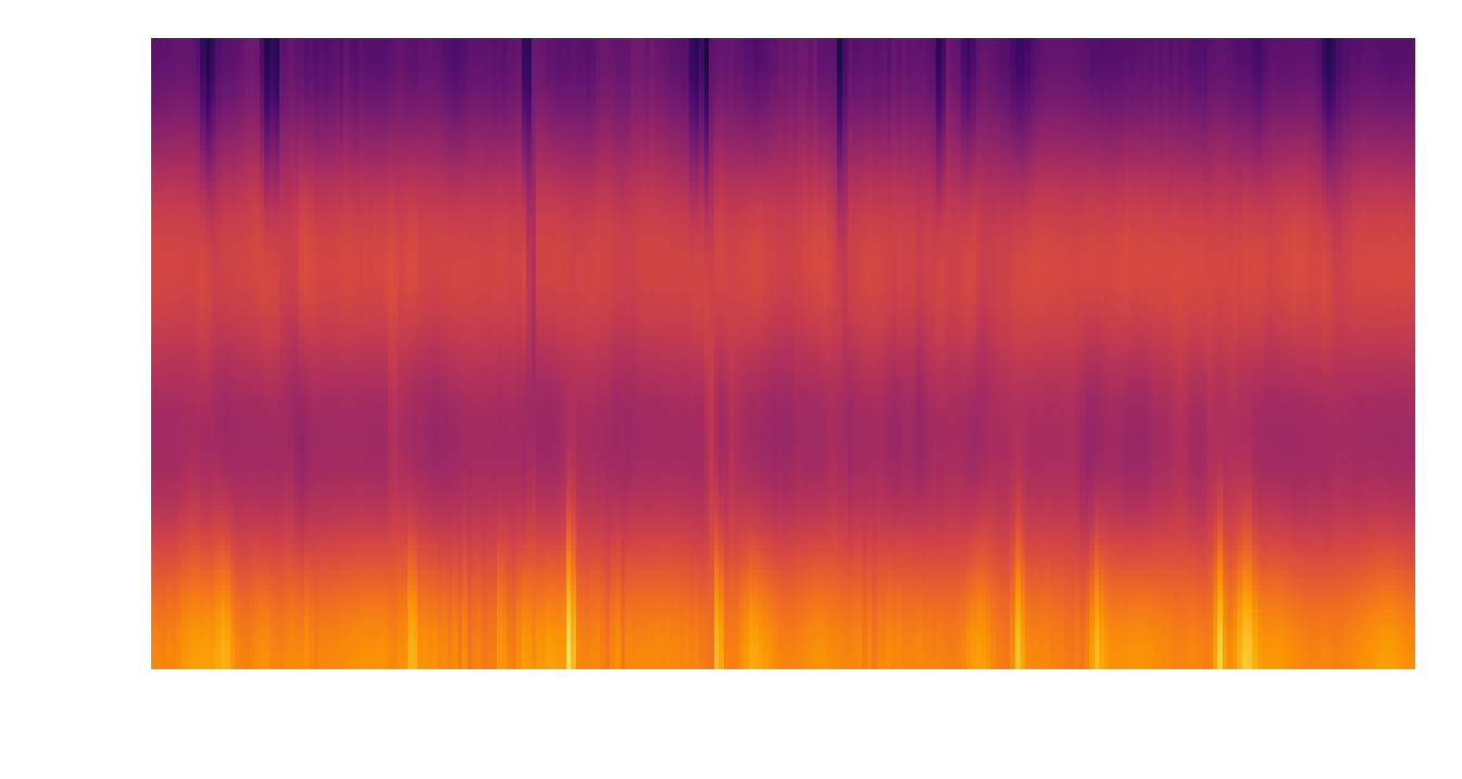 Figure 10
 Figure 11
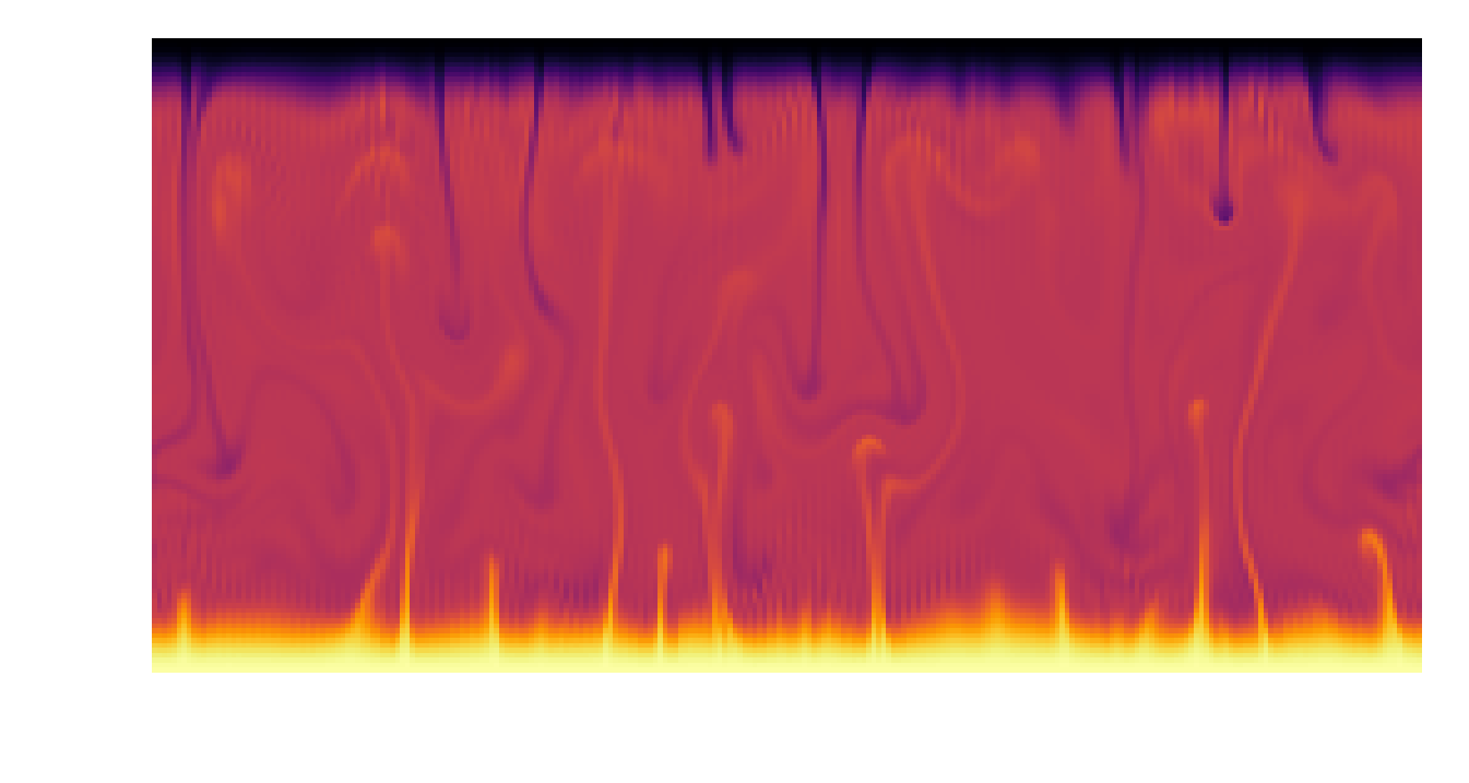 Figure 12
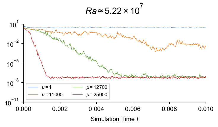 Figure 13
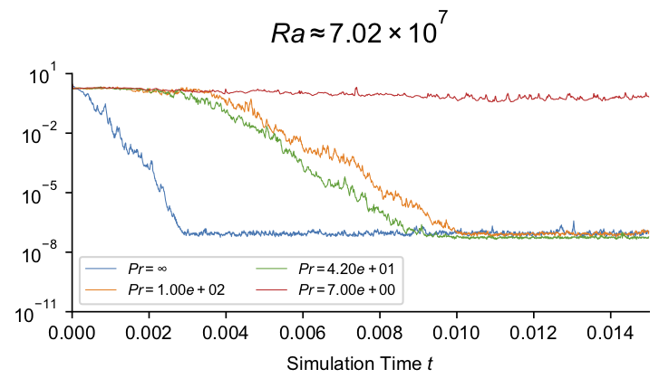 Figure 14
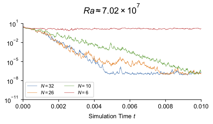 Figure 15
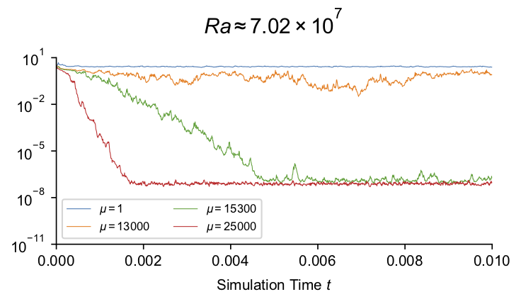 Figure 16
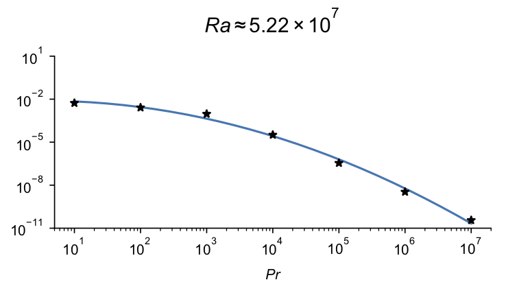 Figure 17
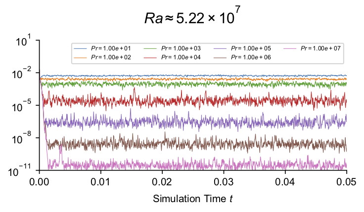 Figure 18
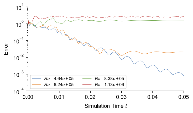 Figure 19
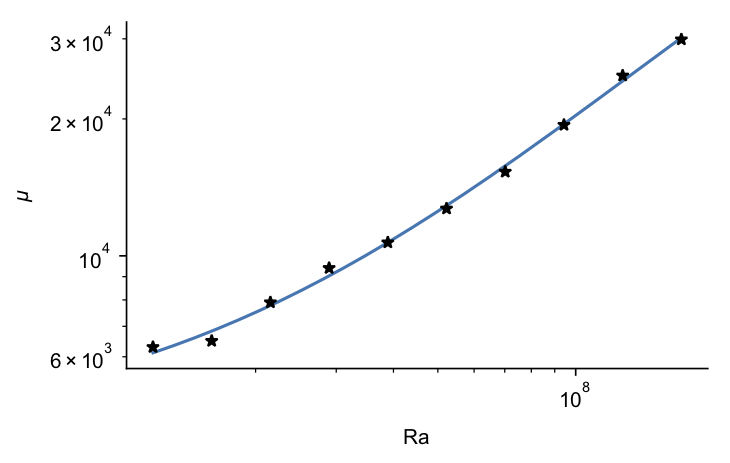 Figure 20
| 75 | ||
| 56 | ||
| 56 | ||
| 100 | ||
| 42 | ||
| 42 | ||
| 42 | ||
| 31 | ||
| 31 | ||
| 31 |
Peer Reviews
No public reviews on file for this paper yet. If you reviewed it on a platform where reviews are public (OpenReview, ICLR, NeurIPS, ICML), you can paste yours below so the community can read it here.
Code & Models
Videos
No videos yet. Explain this paper in a talk, walkthrough, or lecture? Add one.
Data Assimilation in Large-Prandtl Rayleigh-Bénard Convection
from Thermal Measurements
A. Farhat, N. E. Glatt-Holtz, V. R. Martinez, S. A. McQuarrie, and J. P. Whitehead
emails: [email protected], [email protected], [email protected],
[email protected], [email protected]
Abstract
This work applies a continuous data assimilation scheme—a particular framework for reconciling sparse and potentially noisy observations to a mathematical model—to Rayleigh-Bénard convection at infinite or large Prandtl numbers using only the temperature field as observables. These Prandtl numbers are applicable to the earth’s mantle and to gases under high pressure. We rigorously identify conditions that guarantee synchronization between the observed system and the model, then confirm the applicability of these results via numerical simulations. Our numerical experiments show that the analytically derived conditions for synchronization are far from sharp; that is, synchronization often occurs even when the conditions of our theorems are not met. We also develop estimates on the convergence of an infinite Prandtl model to a large (but finite) Prandtl number generated set of observations. Numerical simulations in this hybrid setting indicate that the mathematically rigorous results are accurate, but of practical interest only for extremely large Prandtl numbers.
**Keywords: Data Assimilation, Rayleigh-Bénard Convection, Large Prandtl Limit
MSC2010: 76E06, 62M20, 35Q35 **
Contents
- 1 Introduction
- 2 The Rayleigh-Bénard System and Nudging Equation
- 3 Mathematical Background
- 4 Infinite-Prandtl Assimilation
- 5 Finite-Prandtl Assimilation
- 6 A Scenario of Model Error
- 7 Conclusions and Outlook
- Acknowledgments
1 Introduction
In order to make accurate predictions, numerical models for geophysical processes require establishing accurate initial conditions. Data assimilation is used to estimate weather or ocean (or any other geophysical) variables by incorporating the real world data into the mathematical system to obtain an accurate initialization. One of the classical methods of data assimilation, see, e.g., [HA76, Dal91, LBM91, LSN82, VH89, SS90, ZNLD92, SB93, VLDP03, AB08, BLSZ13, AOT14], is to insert observational measurements directly into a model as the latter is being integrated in time (also known as nudging or newtonian relaxation). There is a significant amount of recent literature concerning the mathematically rigorous analysis of nudging algorithms for data assimilation developed for hydrodynamic equations with a particular focus on weather and climate systems. Recently, a nudging scheme, known as 3DVAR, was studied in [BLSZ13] in the case where observables are given as noisy Fourier modes, and in [AOT14], which successfully accommodates a larger class of observables that, in particular, includes the more physically relevant cases of nodal values and volume elements; see also [BOT15], where observational error is accounted for. In these articles, rigorous proofs are obtained for the synchronization of the approximating signal with the true signal that corresponds to the observations, using the two-dimensional (2D) incompressible Navier-Stokes equations (NSE) as a paradigm.
The data assimilation algorithm analyzed in [BLSZ13, AOT14] can be described as follows: suppose that represents a solution of some dynamical system governed by an evolution equation of the type
[TABLE]
where the initial state of the system, , is unknown. We would like to accurately track this solution as increases notwithstanding our uncertainty in . Let represent an interpolant operator based on the observations of the system at a coarse spatial resolution of size , for . We then construct a solution from the observations that satisfies the equations
[TABLE]
where is a relaxation (nudging) parameter and can be prescribed as an arbitrary initial condition. We then take as prediction of which we anticipate becomes more accurate as (and therefore the amount of observed data ) increases.
The algorithm designated by (1.2) was designed to work for dissipative dynamical systems of the form (1.1) that are known to have global-in-time solutions, a finite-dimensional global attractor, as well as a finite set of determining parameters (see, e.g., [FP67, FT84, FT91, JT92b, JT92a, CJT97, HT97, FMRT01] and references therein). Typically in these settings, following the ideas in [FP67], lower bounds on and upper bounds on can be derived such that the approximate solution converges to the reference solution as . This was initially demonstrated for the 2D Navier-Stokes equations in [BLSZ13, AOT14].
Numerous further studies, both analytical and numerical, have been carried out for the algorithm (1.2), illustrating its broad scope of applicability. For instance, the nudging approach has been validated for models including the 2D magnetohydrodynamic system [BHLP18], the 2D surface quasi-geostrophic equation [JMT17], three-dimensional (3D) Brinkman-Forchheimer-Extended Darcy model [MTT16], and 3D simplified Bardina model [AB18]. The practically and physically relevant scenarios of discrete-time and time-averaged observables was studied in [FMT16, BMO18, JMOT18]; more recently, it was shown in [BFMT18] that this nudging algorithm is capable of synchronizing the statistics propagated by the flow as they are observed only on a coarse-mesh scale; the efficacy of this algorithm for assimilating actual data sampled from a regional domain encompassing most of Northern Africa and the Middle East was recently tested in [DDL*+*18]. We refer the reader to [Dal91] for a summary on the use of data assimilation in practical forecasting and [Kal03] for a comprehensive text on numerical weather prediction where nudging has been employed.
Regarding related numerical studies, [GOT16] demonstrated in the case of the 2D NSE that the number of observables required for synchronization using (1.2) is much lower in practice than what has been deemed sufficient by the rigorous analysis. In the setting of the 2D RB system, numerical studies were carried out in [ATG*+*17], and then in [FJJT18] for nearly turbulent flows using vorticity and local circulation measurements. We emphasize that the numerical experiments carried out in the present article are for moderately turbulent flows whose dynamics are significantly more complex than the regime of two-cell convection rolls that [ATG*+*17] was restricted to. Moreover our studies are carried out to a similar high degree of numerical precision as found in [FJJT18]. We refer the reader to [ANLT16, FET17, DLMB18, CHL18] for various other studies in the context of turbulent flows such as how one can leverage the nudging scheme to infer unknown parameters of the flow. In [BM17, IMT18, MT18] analytical studies on the various modes of synchronization of the algorithm (1.2) and on certain variants on its numerical discretization were carried out.
The earth system is heated from within and cooled by the atmosphere or ocean at the earth’s surface. On geological time scales the mantle’s motion can be modeled as a fluid. The big difference between the temperature of the top mantle and the bottom mantle is a major source of the convective motion (fluid motion driven by temperature difference). The full compressible, temperature-dependent viscous equations of motion that ostensibly describe flow in the mantle [TS14] are currently beyond the reach of a rigorous mathematical analysis, but a first order approximation to this system is adequately described by taking the infinite Prandtl limit [Wan04a, Wan04b, Wan05, Wan07, Wan08a, Wan08b, FGHR15] of the Rayleigh-Bénard (RB) system first described in [Ray16] by Lord Rayleigh. We recall that the Prandtl number represents the ratio of the kinematic viscosity to the thermal diffusivity. Since the original formulation of the minimal mathematical model in [Ray16], extensive research has sought to quantify its dynamical evolution, [Lor63, Ahl74, AB78, BdBAC91], and resultant large spatial and long temporal scale impact of convective flow, see [AGL09, LX10] for example. Despite the seeming simplicity of the RB system, there remains open questions regarding the exact nature of the convective heat transport, and the impact and nature of boundary layers at physically relevant values (see e.g. [AGL09]). To further complicate matters, mantle convection is far more nuanced than Rayleigh-Bénard convection, having several other unanswered questions, in addition to the well-known open problems in the latter setting. Unlike the low Prandtl number setting, experimental investigations of mantle convection are not practical, so numerical simulations provide one of the only avenues to investigate these issues. Of fundamental concern in such simulations is the dependence of the simulation on the initial condition and/or true physical setting, which would ideally be accompanied by physical observations. The collection of observational data from the mantle is an onerous inverse problem that obfuscates much of the desired resolution in time and space [TS14], both in the sense of physical accessibility, and due to the relevant time scales involved. Indeed, the evolution of the mantle is on millenial time scales. Despite remarkable advances in imaging technologies, observations of the mantle are sparse and prone to noise and are insufficient to determine the mantle’s state. Thus, the development of the advanced real-time prediction systems that are capable of depicting and predicting the mantle’s state is necessary to gain insight into the dynamics in the earth’s interior.
Access to observations from earth’s mantle is limited. Geophysicists have decent observations at the surface (top layer) of plate velocities and heat flow distribution and have probes of mantle temperature where volcanism occurs. Since the motion of the tectonic plates is very slow (the relative movement of the plates typically ranges from zero to 100 mm annually), we can assume that the top plate is stationary and with fixed temperature. Thus, a realistic forecast model for the dynamics of earth’s mantle will employ sparse thermal observations only. In the context of atmospheric and oceanic physics, data assimilation algorithms where some state variable observations are not available as an input, have been studied in [CHJ69, EB87, GSY77, GHA78] for simplified numerical forecast models. Particularly related to the study carried out in this article, it was shown in the case of the 2D NSE [FLT16a] and the 2D RB system in [FLT17] that measurements on just a single component of velocity is sufficient to obtain synchronization. Charney’s question in [CHJ69, GHA78, GSY77] asks whether temperature observations are enough to determine the entire dynamical state of the system. In [GSY77], an analytical argument suggested that Charney’s conjecture is correct, in particular, for a shallow water model. Further numerical testing in [GHA78] affirmed that it is not certain whether assimilation with temperature data alone will yield initial states of arbitrary accuracy. The authors in [ATG*+*17] concluded that assimilation using coarse temperature measurements only will not always recover the true state of the full system. It was observed that the convergence to the true state using temperature measurements only is actually sensitive to the amount of noise in the measured data as well as to the spacing (the sparsity of the collected data) and the time-frequency of such measured temperature data. Rigorous justification for Charney’s Conjecture was provided in [FLT16c] in the case of the 3D Planetary Geostrophic model. Earlier, for the specific setting of 3D convection in a porous medium, where inertial effects can be ignored in the fluid velocity, it was shown in [FLT16b] that temperature measurements alone suffice to determine the velocity field. By comparison, the thrust of the analysis performed here is to establish the conclusions analogous to [FLT16b] while accounting for these inertial effects within the regime of a finite but large Prandtl number.
We consider the nudging approach both analytically and through numerical experiments to explore the range of applicability of the technique in this geophysically interesting context of large Prandtl convective systems. Ultimately, we accomplish the following:
We develop a nudging data assimilation scheme for both large and infinite Prandtl number Rayleigh-Bénard convection in the traditional simplified three-dimensional box geometry (cf. (2.4),(2.5) and (2.9) below) with observations in the temperature field only. In Section 2 we formally introduce the governing equations for the 3D RB system and then in Section 3, we provide the mathematical framework within which our analysis is performed, as well as the relevant well-posedness results for the 3D RB system. We then establish rigorous estimates on the convergence rates for the simpler case of in Section 4. The case of large, but finite is addressed in Section 5. 2. 2.
Perform high-resolution direct numerical simulations (DNS) on the two-dimensional version of this problem for moderately turbulent flows, in an effort to shed some light on the practical applicability of the rigorous estimates. In particular, we probe the values of the relaxation parameter and the number of required modes for the nudging scheme to converge. This is done in Sections 4.2 and 5.2, immediately after their respective mathematical analysis. 3. 3.
Consider a practical scenario of ‘model error’, in which the assimilated variables are nudged “incorrectly.” Specifically, we assume that the modeling system corresponds to the infinite Prandtl system nudged by data corresponding to a finite Prandlt system (2.4), (2.5). This situation is studied both analytically and numerically in Section 6.
We note that the choice of finitely many Fourier modes as the manifestation of our observables is made for ease of both exposition and numerical implementation. We reserve establishing estimates on the convergence rates for more general observables to a subsequent study.
2 The Rayleigh-Bénard System and Nudging Equation
This initial section recalls the Rayleigh-Bénard (RB) system and its non-dimensional formulation. We then present the precise form of the nudging algorithm which we will study in the sequel.
The Rayleigh-Bénard system for convection originates from the Boussinesq equations for an incompressible fluid with appropriate boundary conditions. The Boussinesq system over a -dimensional domain, where , , is given by
[TABLE]
where is the velocity vector field, is the scalar pressure field, and denotes the temperature of a buoyancy driven fluid. The parameter denotes the kinematic viscosity of the fluid, its thermal diffusivity, the thermal expansion coefficient, denotes the constant gravitational force and is a constant vector anti-parallel to the gravitational force. To model convection, (2.1) is then supplemented by the boundary conditions
[TABLE]
where is a fixed constant determined by the (relative) strength of the bottom heating. The relations (2.1), (2.2) together constitute the 3D RB system for convection. We note that variations on these boundary conditions are applicable to the earth’s mantle, but as our focus is on the convergence of the data assimilation scheme, we assume that such variations have secondary effects.
Non-dimensionalized variables
As is customary, we work with non-dimensionalized variables. The system (2.1) is rescaled using as a length scale, as the temperature scale, and the diffusive scale as the time scale. The relevant non-dimensional physical parameters for the system are the Prandtl number, , and Rayleigh number, , which are defined as
[TABLE]
This leads to non-dimensionalized variables over the rescaled domain , , which satisfy
[TABLE]
with the boundary conditions
[TABLE]
For notational simplicity, we will drop the ′ in all that follows.
As previously alluded to, the physical setting of interest in this article is the earth’s mantle where the Prandtl number is large, namely, on the order of . Upon formally setting in the system (2.4)–(2.5), one arrives at
[TABLE]
We note that the initial velocity is then determined by and the corresponding momentum equations. Although there are several additional physical effects relevant to mantle convection that are omitted from the Rayleigh-Bénard model considered here, we consider (2.9) to be an appropriate “zeroth order” representation of mantle convection; it provides the starting point and test model for mantle convection simulations (cf. [BBC*+*89]). Although we anticipate eventually extending the results of the current investigation to more realistic models of mantle convection, we believe a more in-depth understanding of the problem at hand is a necessary first step.
Nudging setup
The idea, following [BLSZ13, AOT14] and sketched in the introduction, is to nudge the assimilated system as in (1.2) with a projection of the ‘truth’ that represents the exactly realizable observations of the original system. More precisely, the nudging is accomplished by introducing an affine feedback control term to the original ‘forecast’ model (1.1), whose purpose is to enforce the asymptotic convergence of the solution of the assimilated system (1.2) towards that of the original system (1.1), but only on the scales at which the observations are made; it is this ‘relaxed’ imposition that ensures the practicality of the nudging scheme. For this article, our ‘truth’ is assumed to be represented by (2.4), (2.5) or by (2.9).
Let satisfy (2.4), (2.5) over , from which we have obtained partial observations in the form of finitely many Fourier coefficients corresponding to wave-numbers , for some integer . Let denote the assimilated or modeled system variables, which satisfies
[TABLE]
where denotes the projection onto Fourier wave-numbers (see (3.8) below). Its infinite Prandtl counterpart is given by
[TABLE]
where comes from either (2.4), (2.5) or (2.9).
One of the basic goals of this paper is to show that and as in the appropriate space for specific conditions on and the number of projected modes relative to and . This indicates that for specified Rayleigh and Prandtl numbers one can determine a sufficiently large number of modes and a sufficiently large nudging parameter to ensure that the assimilated system will asymptotically match the true system.
3 Mathematical Background
For the sake of completeness, this section presents some preliminary material and notation commonly used in the mathematical study of hydrodynamic systems, in particular in the study of the NSE and the Euler equations for incompressible fluids. For more detailed discussion on these topics, we refer the reader to, e.g., [CF88, Tem97].
Let , where and we denote the spatial variable . We consider the function spaces
[TABLE]
where and denote the classical Sobolev class of first-order and second-order weakly differentiable functions over , respectively. We use the notation to denote the -fold product of a set , and to denote the usual inner product over ,
[TABLE]
for , and . The inner product on , , is given by
[TABLE]
where is a multi-index and . The spaces are then endowed with a Hilbert space structure, whose respective inner products are given by
[TABLE]
The spaces have analogous Hilbert space structures. We denote by and the dual spaces of , and , respectively. We then have the following continuous injections:
[TABLE]
In what follows we will denote the norm by . For all other Banach spaces , e.g. , for , etc., we denote the associated norms explicitly as .
Let
[TABLE]
denote the orthonormal eigenpairs corresponding to the Laplace operator on the domain supplemented with the mixed horizontally periodic-vertically Dirichlet boundary condition as in (3.1). Then each can be expressed in terms of the eigenfunctions as
[TABLE]
and the eigenfunctions satisfy the orthogonality relation
[TABLE]
For each , define the projections by
[TABLE]
where is the identity operator. In other words, is a truncation of the eigenfunction expansion, and is its orthogonal complement. The orthogonality of the eigenbasis yields the identities
[TABLE]
for any .
We next recall the following well-known a priori estimates for Stokes’ equations
[TABLE]
cf. [CF88] and the drift-diffusion equation, (3.15) where the advecting velocity field is divergence free as in e.g. [Tem97, Wan05]. We adapt these results here to our notation and setting as follows
Lemma 3.1**.**
Let and . There exists a unique and (up to constants) such that (3.11) is satisfied. Moreover, there exists a constant such that
[TABLE]
The next lemma follows from the theory of linear transport equations in [DL89] and a variant of the maximum principle proved in [FMT87] .We will refer to the following notation for the “positive” and “negative parts” of a function:
[TABLE]
Lemma 3.2**.**
Let and . Let and be a.e. -periodic in and (in the sense of trace). Suppose that satisfies
[TABLE]
where the boundary values on are interpreted in the sense of trace. Then there exists a constant and functions such that and satisfy
[TABLE]
for all .
For the system (2.9), when , the velocity field, , is determined by the evolution of . The well-posedness of this system then follows in a standard way, for either dimension , and its solution satisfies the estimates stated in Lemma 3.1 and 3.2. We formally state this result as the following theorem.
Theorem 3.1**.**
Let . Suppose that is a.e. in , that is a.e. -periodic in and (in the sense of trace). Then there exists a unique satisfying (2.9) such that
[TABLE]
for all . Moreover, there exist positive constants and , such that
[TABLE]
for all , where .
We consider a change of variable, denoted by , that represents the fluctuation of the temperature around the steady state background temperature profile :
[TABLE]
The functional setting determined by (3.2)-(3.4) accommodates a rigorous mathematical analysis for the perturbed variable . The results derived for are then transferred naturally to the desired results for the original variable . We appeal to [Wan05, Wan07] for the global existence and eventual regularity of suitable weak solutions for (2.4)-(2.5), as well as the existence of the “global attractor” for the dynamics, although we will not make explicit use of this fact in this article. We will also say that a solution of (2.4), (2.5) is regular on if . If , we say that the solution is a global regular solution.
Theorem 3.2** ([Wan05, Wan07]).**
Let . Recalling the notation (3.2)–(3.4) let and .
- (i)
(Global Existence of Weak Solutions) For any , there exists such
[TABLE]
where is related to by the relation (3.16). This satisfies (2.4)–(2.5) in the usual weak sense, and maintains the initial condition . Moreover, the following energy inequality and maximum principle are satisfied for all :
[TABLE]
where are defined as in (3.14). 2. (ii)
(Eventual Regularity of Weak Solutions) There exists a constant such that if , then there exists a time for which all suitable weak solutions corresponding to become regular solutions on . In particular, when , there exist constants and , depending on , such that
[TABLE]
for all .
For the remainder of the article, we will therefore assume that , have evolved for a sufficiently long time, so that is a regular solution to either (2.4)–(2.5) or (2.9). Physically speaking, the set-up of our study assumes that reality is represented exactly by a solution to (2.4)–(2.5) or (2.9) and that we have been observing the system after the point in time at which it has become globally regular. Thus, for the purposes of our analysis, we will henceforth make the following standing hypotheses for the remainder of the paper.
Standing Hypotheses.
Let and . Let be the constants from Theorem 3.1. When , we assume:
a.e. periodic in and , (in the sense of trace); 2.
; 3.
is the unique global solution to (2.9) corresponding to and guaranteed by Theorem 3.1. In particular, satisfies
[TABLE]
for all .∎
On the other hand, let , , and be the constants in Theorem 3.2 . When , we assume:
; 2.
is the unique regular solution to (2.4), (2.5); 3.
When , satisfies
[TABLE]
for all . 4.
When , satisfies
[TABLE]
for all , where , .∎
Remark 3.1**.**
Since we have non-dimensionalized our variables, we point out that although the bounds in are derived for the case , they are also valid for the case , up to constants, provided that , which have have assumed as one of our standing hypotheses.
4 Infinite-Prandtl Assimilation
We will first treat the Data Assimilation problem for the infinite Prandtl number system (2.9), (2.17). Hence, throughout this section we assume that , i.e., holds.
A rigorous mathematical analysis is performed in dimensions , while the numerical component of our studies are carried out for . Due to the structure of the nudged system (2.17), we do not have a maximum principle. Instead, we require only that (2.17) have a well-defined solution in the weak sense, which one can do by establishing that the differences , satisfy their respective evolution in the weak sense. Since one of the relevant a priori estimates to this end are performed below for the proof of Theorem 4.2, we simply state this result as the following theorem.
Theorem 4.1**.**
Let and be as in (3.7). Let a.e. in such that is a.e. -periodic in with (in the sense of trace). Suppose satisfies . Then there exists a unique satisfying (2.17) in the weak sense such that
[TABLE]
*for all . *
4.1 Synchronization
We are now ready to state and prove the main theorem of this section. We show that (2.9) and (2.17) synchronize under certain conditions detailed below.
Theorem 4.2** (Infinite-Prandtl Synchronization).**
Let and be as in (3.7). Let satisfy and be given as in Theorem 4.1. Let be the corresponding unique solution to (2.17) guaranteed by Theorem 4.1. There exists a constant such that if
[TABLE]
then for all
[TABLE]
for .
Proof.
Let , , and . Subtracting (2.9) from (2.17) yields the system
[TABLE]
with the initial condition . The momentum equation in (4.6) satisfies Lemma 3.1, so there exists a constant such that
[TABLE]
Therefore, to establish (4.2), it is sufficient to show that with an exponential rate in .
Upon multiplying the equation in (4.6) by and integrating over , we obtain
[TABLE]
Assume that is chosen sufficiently large so that (4.1) holds, where is, as of yet, unspecified. After integrating by parts, an application of the Sobolev embedding , (4.7), and then of the Standing Hypotheses imply
[TABLE]
On the other hand, due to (3.10) and the inverse Poincaré inequality, and since satisfies , it follows that
[TABLE]
Joining (4.8) with (4.2) and (4.2) and combining like terms, we arrive at
[TABLE]
Finally, by Gronwall’s inequality and the second condition in (4.1), we deduce that
[TABLE]
which completes the proof upon choosing . ∎
Theorem 4.2 shows that given and reasonable boundary conditions and , we can always choose and large enough so that and eventually match in the infinite-time limit. In the next subsection, we use numerical simulations to verify that this is indeed the case.
4.2 Numerical Results at Infinite Prandtl number
Rather than focusing on a handful of highly turbulent three-dimensional simulations, for the same computational cost we consider more detailed and extensive simulations in the two-dimensional setting where with coordinates in order to search through the relevant parameters. We simulate (2.9) and (2.17) using a stream function formulation with Dedalus [BVO*+*16], a Python package that uses pseudospectral methods to solve partial differential equations on spectrally representable domains. All of the simulations in this section and all that follow are completed with a 4-stage 3rd order Runge-Kutta implicit-explicit time stepping scheme that treats the linear terms implicitly and the nonlinear terms explicitly. Each simulation runs with and Fourier grid points in the horizontal and Chebyshev points in the vertical with a standard dealiasing. All simulations were run until the time-averaged Nusselt number and other pertinent statistics were temporally well-converged for all cases considered here.
Choosing the initial conditions and in our numerical experiments is nontrivial. For , we have two options.
- •
Set for some small perturbation function . This begins the simulation close to the conductive state , which—though not physically relevant—is a suitable starting point for initial experiments.
- •
Load from the final state of a previous simulation with similar parameters. If this previous simulation has run long enough, will thus begin in a reasonable state for the new set of parameters.
Finding a suitable choice for is even less obvious. Setting assumes no prior knowledge of , and results in an overly stiff initialization due to the strength of the initial temperature difference, and is therefore numerically impractical. In addition, initiating at this conductive state ignores observations taken at the initial time which would not be advantageous in practice. On the other hand, setting for large results in a very weak temperature difference so that (2.9) and (2.17) are nearly synchronized at . As a compromise, we set as a low-mode projection of such as . This permits some initial knowledge of the true state without driving it directly to the ‘truth’ immediately.
Values of the Rayleigh number that are of interest for mantle convection are typically between and [TS14, BBC*+*89]. However, the greater value for , the more computationally expensive the simulation, and it is numerically unstable to start in a state such as at large . We therefore select logarithmically spaced values from to and run a simulation for each , one after another. For the very first simulation (), we set , as discussed above, and evolve the systems forward until reaching a nearly steady state. Thereafter, we set as the final from the previous simulation and increment increase . This yields realistic initial conditions for any given in the range considered. Figure 1 shows an example of and , together with subsequent end states of and for .
To measure the synchronization of (2.9) and (2.17), we keep track of the , , and norms of and throughout the simulation. Each error is normalized by dividing by the norms of the truth system’s variables. For example, to measure the temperature difference in , we compute at each simulation time . For simplicity, we write these errors without the denominators in all that follows.
Figure 2 shows how the tracked error norms decrease in the simulation from Figure 1. Though the analysis indicates that these norms should converge to , seeing the errors decrease to about is numerically satisfactory in this setting, given the format in which the norms are calculated, i.e. some errors do accumulate in the calculation of the norm itself.
4.2.1 Dependencies of nudging parameter
Previous studies, [ATG*+*17, FJJT18], of data assimilation for Rayleigh-Bénard convection fixed the value of the nudging parameter at in their experiments and instead focused on the effects of other parameters, such as the number of projected modes. However, Theorem 4.2 requires that be proportional to , so we do not expect synchronization with as increases. Indeed, Figure 3 shows that for in the range of to , using results in either extremely slow convergence, or in no convergence at all.
To explore the relationship between , , and needed for synchronization to occur, we fix two of the parameters at a time and run several simulations with various values for the remaining parameter. First, we fix , set , and vary until synchronization can be observed within units of simulation time (a simulation of this length usually requires several thousand iterations). Table 1 records the smallest value of where synchronization was observed; Figure 4 shows the convergence rates for a few different values when and .
Given the requirement (4.1) from Theorem 4.2, it is surprising to discover that—based on Table 1—the relationship between and is more linear than quadratic. Indeed, a least squares fit of the data to a general quadratic of the form yields coefficients of , , and (essentially ). See Figure 5.
4.2.2 Relation between relaxation and number of observables
The relaxation parameter is a system parameter without a clear physical interpretation. The number of projected Fourier modes , on the other hand, indicates the amount of data that is “visible” to the assimilating system. Therefore, a lower bound on represents how much data is required in order to maintain an accurate model. Fixing as given by Table 1, we decrease to see how it affects synchronization. See Figure 6. Note that as expected, the less modes retained in the projection, the slower synchronization is achieved, and if a sufficiently low number of modes () is observed then synchronization never occurs. In Table 2 we summarize our findings concerning the number of modes needed as a function of (given a suitably large choice for ).
4.2.3 Summary
The numerical simulations verify that over physically relevant values of , we can pick large enough to nudge (2.9) toward (2.17); in particular, the experiments confirm Theorem 4.2 and show that the conditions stated therein are stronger than necessary. Furthermore, synchronization can be obtained with a relatively low number of modes even for large , as long as is chosen large enough. We took the approach of varying first and then , but it is just as feasible to vary for a fixed and .
5 Finite-Prandtl Assimilation
We now turn to the case when is finite, but large. Thus, throughout this section, we will assume that , so that we automatically have that holds.
As in Section 4, we first state the relevant well-posedness result for the nudged equation. We then rigorously establish synchronization of the nudged signal with the true signal, then proceed with a numerical study for the two-dimensional setting.
It is not immediately clear how to properly adapt the argument for (2.9)–(2.17) in [Tem97, Wan05] to establish a maximum principle (see Lemma 3.2) for the assimilating variable due to the presence of the additional term in (2.17) (cf. [JMST18] for a case where it is necessary to develop a maximum principle in spite of this term). However, since we are assuming is a regular solution to (2.4)–(2.5), it is straightforward to verify global existence and uniqueness for the associated nudged system by instead considering the corresponding system for the difference , where and . In this setting, we need only appeal to a maximum principle for , rather than for . The well-posedness of the nudged system then follows in a standard fashion, so that we opt to only state the result here and refer the reader to [FJT15] for the appropriate details.
Theorem 5.1**.**
Let and be as in (3.7). Let . Suppose satisfies . Then there exists a unique solution satisfying (2.13) such that
[TABLE]
for all .
5.1 Synchronization
We will establish the finite Prandtl analog to Theorem 4.2. For this, it will be convenient to establish the following stability estimate first.
Lemma 5.1**.**
Assuming the conditions of Theorem 5.1, there exists a constant such that if
[TABLE]
then
[TABLE]
holds for .
Proof.
Similar to the analysis performed for Theorem 4.2, we consider the solution to the difference system
[TABLE]
Then, multiplying the second equation by integrating and arguing as in (4.2) we obtain
[TABLE]
On the other hand, an analogous energy calculuation for yields
[TABLE]
We estimate the right hand side of (5.7) using Hölder’s inequality, the Gagliardo-Nirenberg interpolation inequality, and Young’s inequality to obtain
[TABLE]
Next, for in (5.8), we have from Hölder’s inequality, the Sobolev embedding , Gagliardo-Nirenber interpolation inequality, and Young’s inequality that
[TABLE]
For , we use the Cauchy-Schwarz inequality to obtain
[TABLE]
Combining the bounds for -, we have
[TABLE]
Thus, by the second condition in (5.1), it follows that
[TABLE]
Therefore, by Gronwall’s inequality the desired bound (5.2) now follows. ∎
Theorem 5.2**.**
Assume the conditions of Lemma 5.1. There exists a constant such that if
[TABLE]
then
[TABLE]
*holds for all , where . *
Proof.
By of the Standing Hypotheses, it follows that
[TABLE]
By and the Sobolev embedding, , it follows that
[TABLE]
Now upon combining (5.12), (5.13), it follows that there exists such that
[TABLE]
Then, having chosen according to (5.10), upon taking square roots, we deduce (5.11) from and Lemma 5.1, as desired. ∎
Remark 5.1**.**
Observe that (5.10) requires the Prandtl number to be very large to ensure that synchronization occurs. Indeed, for this condition indicates that which would place the Prandtl number in a regime beyond the one that occurs for the earth’s mantle. In addition, the lower bound on stated here would imply that which would yield a very stiff problem numerically, particularly if as indicated. Gratefully, as seen in the next subsection, these rigorous estimates are pessimistic, and synchronization is achieved for much lower values of and than are indicated here.
5.2 Numerical Results
The numerical results are similar to those presented in Section 4.2, i.e. the same spatial discretization and time-stepping algorithm are employed here, but now we also consider variations in . In addition, for finite the velocity field is no longer slaved directly to the temperature field, requiring us to specify an initial condition for the velocity as well as the temperature. This is done as in the infinite case by setting the initial state of the assimilated system to a low-order projection of the ‘true’ system. Simulations at higher Rayleigh numbers are initiated with flow fields from previous simulations at incrementally lower . To ensure that the algorithm is working, we first check that synchronization still occurs for reasonable choices of , , and given a finite , say . See Figure 7.
To simplify our exploration, for each value of listed in Tables 1 and 2, we pick so that the systems synchronize quickly. Then, with , we run simulations for logarithmically spaced values of from to . Even with these larger-than-necessary choices of , convergence is lost for small enough . See Figure 8 for a few additional examples and Table 3 for the chosen and the lowest where synchronization still occurs.
There are two main points to take away from these results.
- •
Finite-but-large Prandtl data assimilation through only temperature measurements is possible, though it is slower than the infinite Prandtl setting explored in Section 4.
- •
The relationship between , , , and remains unclear and would require further measurements to precisely quantify. However, the fact that the assimilation works at all with reasonably small indicates that the inequality constraints in Theorem 5.2 are strongly overstated, or that the constants in (5.10) are extremely small.
- •
While the estimates obtained in Theorem 5.2 are clearly pessimistic it is interesting to note that the qualitative behavior is as expected. That is, the finite Prandtl system will synchronize so long as is sufficiently large. This is not unexpected as the limit of will be dominated by inertial effects in which the temperature and velocity field are nearly decoupled so we would anticipate that temperature observations alone will not suffice to recover the full flow field.
6 A Scenario of Model Error
Finally, we address a realistic scenario of assimilating observables that correspond to solutions of the finite, but large Prandtl number system (2.4), (2.5) into the “incorrect,” albeit more computationally tractable, infinite Prandtl data assimilation system (2.17). Thus, we suppose satisfy and simply choose a suitable for (2.17) since the corresponding initial velocity is enslaved by the temperature evolution for the later nudging equation. Before we perform the analysis for the error estimates, we state the well-posedness result corresponding to the nudged equation, whose proof follows along similar lines to that of Theorem 4.1.
Theorem 6.1**.**
Let , and be as in (3.7). Let of (2.4)-(2.5) satisfying . Let a.e. in such that is a.e. -periodic in with (in the sense of trace). Suppose satisfies . Then there exists a unique satisfying (2.17) in the weak sense such that
[TABLE]
*for all . *
6.1 Error estimates
Since our data assimilation equation (2.17) does not correspond to the true evolution of the observables (2.4), (2.5), we do not expect to obtain an exact synchronization. Instead, we derive estimates that quantify the maximal error possible, and which will vanish as the Prandtl number is taken increasingly large.
Theorem 6.2**.**
Let satisfy and be given as in Theorem 6.1. Let be the corresponding unique solution to (2.17) guaranteed by Theorem 6.1. There exists a constant such that if
[TABLE]
then there exist positive constants such that
[TABLE]
for all .
Proof.
Let , , . Then
[TABLE]
Upon taking the -inner product of with (6.3), (6.4), respectively, then adding the consequent relations, we obtain
[TABLE]
Upon applying Hölder’s inequality, the Poincaré inequality, the Sobolev embedding theorem, Ladyzhenskaya’s inequality, and Theorem 3.2 , we derive
[TABLE]
Upon combining estimates for with the conditions in (6.1) and the fact that , it follows that
[TABLE]
Hence, by Gronwall’s inequality, we arrive at
[TABLE]
Lastly, by Lemma 3.1 and of the Standing Hypotheses, we have
[TABLE]
We take the square root of (6.5) and add the result to (6.6) to complete the proof.
∎
6.2 Numerical Results
To numerically verify Theorem 6.2 in a way that is consistent with the numerical simulations corresponding to Theorems 4.2 and 5.2, we compare to . To begin, consider a simulation with , , and . For the finite Prandtl model in Section 5, this set of parameters results in synchronization (see Figure 7). In this situation, however, the synchronization appears to be limited by the error from the model to the reality.
This apparent lack of convergence is expected, however, since Theorem 6.2 only guarantees that the error between and decreases to as time increases. Using the same set of parameters, but with larger and larger , results in tighter and tighter synchronization. To more carefully match the results to the statement of Theorem 6.2, we calculate + at each simulation time . See Figure 10.
While Figure 10 is encouraging, it also highlights a weakness in the data assimilation scheme unique to this hybrid setting. In both the previous settings considered here, the rigorous estimates were pessimistic particularly for the large but finite Prandtl case. It appears that the estimates provided here for this hybrid setting are far more true to practice, i.e. while the error is not linear in as seen in Figure 10 it is certainly dominated by the effects of the Prandtl number. This suggests that the practical success of these types of data assimilation schemes is highly dependent on the data coming from the same model as the simulated system, an unrealistically stringent restriction. Recall that the Boussinesq approximation is effectively a “zeroth order” approximation for the mantle, meaning the true physical system has several complicated secondary effects (some of which are unknown) that are not included in the model. The lack of numerical synchronization in such a simple setting suggests that data assimilation may not be as adaptable to settings where the exact model is not known.
7 Conclusions and Outlook
In Section 4, we examined a data assimilation scheme for the Rayleigh-Bénard system with and showed rigorously that synchronization occurs between the data and assimilating equations under certain conditions on the relaxation parameter and the number of projected modes relative to the Rayleigh number when measurements of the temperature only are observed. That is, as long as there is enough data (i.e., is not too small), can be chosen large enough to guarantee synchronization. Though this is a satisfying theoretical result, the numerical experiments in Section 4.2 show that synchronization often occurs under much weaker conditions on and than Theorem 4.2 requires. In particular, the inequality conditions on is shown to be at least an order of magnitude away from being sharp. In addition, the numerical results also demonstrate situations in which synchronization fails, namely when and/or are not large enough.
Section 5 shows that synchronization in the temperature measurements only and at finite is also possible, although the rate of convergence is slower than with and the relationship between , , , and needed to achieve synchronization remains somewhat ambiguous. As in the case, the conditions imposed on appear quite pessimistic when compared to numerical experiments.
Finally, when the true values are taken from simulations, but the assimilating equations use , the synchronization is highly dependent on , as predicted by the rigorous bounds. This hybrid setting illustrates that the difference between the two systems is dominating the error, rather than the dynamical error in the synchronization process. Although the numerical simulations agree well with the rigorous predictions in this setting, they do indicate a pessimistic outlook for additional settings wherein the exact evolution of the dynamics for a data assimilation system of this type is unknown. In particular as noted above, we have omitted several details in our model of mantle convection that play a vital role in the evolution and may have an effect similar to the difference between finite and infinite . To investigate this further, data assimilation applied to the internally heated convective setting (see [Gol16, WD11, WD12] for example), and possibly the anelastic or compressible convective systems [KLvK*+*10] will be explored.
The current consideration of the difference between the infinite and near-infinite Prandtl number convective systems lends itself to further investigations wherein the assimilating model is different from the physical system wherefrom the observations are obtained. For example, one might consider the effects of imprecisely defined boundary conditions, i.e. what if the observations were obtained from a convective simulation in which the velocity satisfied a Navier-slip condition, but the nudged system was modeled with a no-slip condition? Other variations in the model itself might include slight variations in the geometry between the two systems, and additional terms in the equations themselves such as internal heating mentioned above. The rub of the matter is that data assimilation techniques, if they are meant to apply to physical settings such as weather, climate, and investigations of the earth’s mantle, must consider the fallibility of the model they are relying on, that is do variations in the underlying model itself allow for synchronization of the model with the observed truth?
Acknowledgments
This paper was initiated by conversations between AF and NEGH (and eventually JPW) which took place during a workshop at the Institute for Pure and Applied Mathematics (IPAM), for which all the authors are indebted to IPAM, the National Science Foundation (NSF), and organizers of the program on Mathematics of Turbulence in Fall 2014. NEGH would like to acknowledge the grants NSF-DMS-1816551, NSF-DMS-1313272 and Simons Foundation 515990 which supported this work. SM and JPW acknowledge computational resources and support from the Fulton Supercomputing Laboratory at Brigham Young University where all the simulations were performed, as well as extensive feedback from the dedalus developers (see http://dedalus-project.org/). JPW also acknowledges the hospitality and generosity of the Mathematics Department at Tulane University where some of the finishing touches on this work were carried out.
The reference list from the paper itself. Each links out to its DOI / PubMed record.
- 1[AB 78] G. Ahlers and R.P. Behringer. Evolution of turbulence from the Rayleigh-Bénard instability. Physical Review Letters , 40(11):712, 1978.
- 2[AB 08] D. Auroux and J. Blum. A nudging-based data assimilation method for oceanographic problems: The Back and Forth nudging BFN algorithm. Nonlinear Proc. Geophys. , 15:305–219, 2008.
- 3[AB 18] D.A.F. Albanez and M.J. Benvenutti. Continuous data assimilation algorithm for simplified Bardina model. Evol. Equ. Control Theory , 7(1):33–52, 2018.
- 4[AGL 09] G. Ahlers, S. Grossmann, and D. Lohse. Heat transfer and large scale dynamics in turbulent Rayleigh-Bénard convection. Reviews of Modern Physics , 81(2):503, 2009.
- 5[Ahl 74] G. Ahlers. Low-temperature studies of the rayieigh-bénard instability and turbulence. Physical Review Letters , 33(20):1185, 1974.
- 6[ANLT 16] D.A.F. Albanez, H.J. Nussenzveig Lopes, and E.S. Titi. Continuous data assimilation for the three-dimensional Navier-Stokes- α 𝛼 \alpha model. Asymptotic Anal. , 97(1-2):165–174, 2016.
- 7[AOT 14] A Azouani, E.J. Olson, and E.S. Titi. Continuous data assimilation using general interpolant observables. J. Nonlinear Sci. , 24(2):277–304, 2014.
- 8[ATG + 17] M.U. Altaf, E.S. Titi, T. Gebrael, O.M. Knio, L. Zhao, and M.F. Mc Cabe. Downscaling the 2d Bénard convection equations using continuous data assimilation. Comput. Geosci. , 21:393–410, 2017.
