An Efficient Analytical Evaluation of the Electromagnetic Cross-Correlation Green's Function in MIMO Systems
Debdeep Sarkar, Said Mikki, Yahia Antar

TL;DR
This paper derives exact analytical expressions for the electromagnetic Green's function in MIMO systems, enabling fast and accurate calculation of spatial correlation without numerical integrations.
Contribution
It introduces a comprehensive analytical formulation for the electromagnetic Green's function in 3D MIMO systems, eliminating the need for numerical integration.
Findings
Analytical expressions significantly reduce computation time.
Applicable to arbitrary antenna locations and polarizations.
Enhances accuracy of spatial correlation estimates.
Abstract
In this paper, we completely eliminate all numerical integrations needed to compute the far-field envelope cross-correlation (ECC) in multiple-input-multiple-output (MIMO) systems by deriving accurate and efficient analytical expressions for the frequency-domain cross-correlation Green's functions (CGF), the most fundamental electromagnetic kernel needed for understanding and estimating spatial correlation metrics in multiple-antenna configurations. The analytical CGF is derived for the most general three-dimensional case, which can be used for fast CGF-based correlation matrix calculations in MIMO systems valid for arbitrary locations and relative polarizations of the constituent elements.
Click any figure to enlarge with its caption.
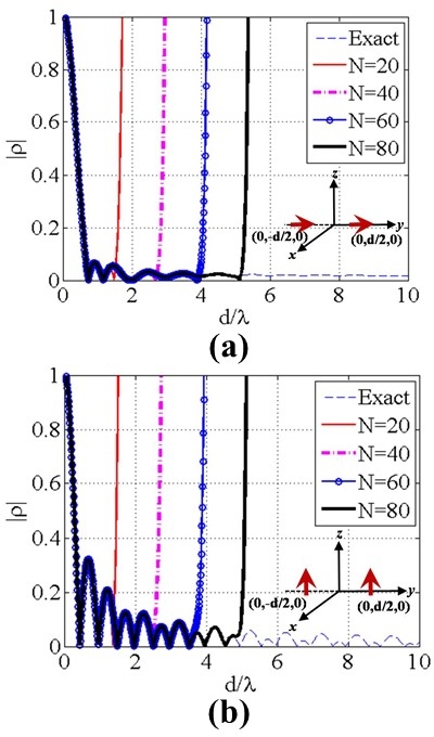 Figure 1
Peer Reviews
No public reviews on file for this paper yet. If you reviewed it on a platform where reviews are public (OpenReview, ICLR, NeurIPS, ICML), you can paste yours below so the community can read it here.
Videos
No videos yet. Explain this paper in a talk, walkthrough, or lecture? Add one.
An Efficient Analytical Evaluation of the Electromagnetic Cross-Correlation Green’s Function in MIMO Systems
Debdeep Sarkar, Member, IEEE, Said Mikki, Senior Member, IEEE, Yahia Antar, Life Fellow, IEEE
Abstract
In this paper, we completely eliminate all numerical integrations needed to compute the far-field envelope cross-correlation (ECC) in multiple-input-multiple-output (MIMO) systems by deriving accurate and efficient analytical expressions for the frequency-domain cross-correlation Green’s functions (CGF), the most fundamental electromagnetic kernel needed for understanding and estimating spatial correlation metrics in multiple-antenna configurations. The analytical CGF is derived for the most general three-dimensional case, which can be used for fast CGF-based correlation matrix calculations in MIMO systems valid for arbitrary locations and relative polarizations of the constituent elements.
Index Terms:
MIMO arrays, Cross-correlation Green’s Function, Infinitesimal Dipole Model (IDM).
11footnotetext: Debdeep Sarkar (Corresponding Author) and Yahia Antar are with the Royal Military College, PO Box 17000, Station Forces Kingston, Ontario, K7K 7B4, Canada (Emails: [email protected]; [email protected]).22footnotetext: Said Mikki is with University of New Haven, West Haven, Connecticut, 300 Boston Post Rd, 06516, USA (Email: [email protected]).33footnotetext: 20XX IEEE. Personal use of this material is permitted. Permission from IEEE must be obtained for all other uses, in any current or future media, including reprinting/republishing this material for advertising or promotional purposes, creating new collective works, for resale or redistribution to servers or lists, or reuse of any copyrighted component of this work in other works.”
I Introduction
Fifth generation (5G) wireless networks aiming at high data-rate ( Gbps) and efficient interference suppression between multiple users in ultra-dense networks (UDNs), deploy large antennas arrays/massive multiple-input-multiple-output (MIMO) systems as key enabling technology [1]-[6]. One crucial aspect of such multiple-antenna systems in MIMO transceivers is the latter’s “spatial correlation matrix”, which accounts for mutual interaction (conventionally, only far-field is taken into account) between the constituent antenna element-pairs [7]-[11]. Despite the pivotal role of this spatial correlation matrix in shaping the overall channel matrix and consequent capacity/interference-suppression issues (see [12]-[15] for details), the impact of pure antenna effects and various core electromagnetic aspects in MIMO channel modelling are often not emphasized adequately.
Traditionally, this antenna spatial correlation performance is determined from a formula involving the radiation patterns of individual elements [10], which makes it very cumbersome to perform antenna current level optimization aiming at a desired diversity performance. To relate the antenna correlation directly to the radiating antenna current distribution (i.e., essentially bypassing altogether the original far-field pattern route), the concept of cross-correlation Green’s functions (CGFs) was first introduced in [16],[17] and later elaborated for antenna design applications [30], [18]. A preliminary step of this CGF-based correlation calculation is to construct a suitable infinitesimal dipole model (IDM) for the radiating MIMO antenna current distribution (see [19]-[28] for detailed theory and applications of IDM). The next step is to employ suitable CGFs in order to compute individual ID-pair interactions systematically and then combine them togethoer to construct the global correlation matrices of the system [16]. Application of CGFs to realize high diversity gain MIMO antenna arrays as well as dual-polarized massive MIMO systems has been reported in recent past [29]-[32]. By efficient integration of the CGFs with finite-difference-time-domain (FDTD) computational paradigm, one can also perform wide-band time-domain correlation analysis for arbitrary antennas [33]-[34]. The CGFs are also extended to deal with radiators involving both electric/magnetic current sources [35]. Possible application of the CGF methodology for near-field stochastic systems [36] and antenna directivity analysis [37] are also being actively explored presently.
However, calculation of the CGF tensor components requires numerical integration involving elevation () and azimuth () angle dependent terms in the argument of complex exponential functions [16], [33]. Therefore, it becomes extremely difficult to efficiently embed these CGFs in fast optimization routines aiming at finding optimum current distributions for desired diversity performance. This necessitates a robust analytical evaluation scheme for the determination of the CGF tensor components and the possibility of achieving this was in fact already suggested in [16]. Although some specialized approximation formulas of the time-domain CGFs were attempted in [38], IDM-synthesis of MIMO antennas strictly requires frequency-domain CGFs, and the analytical evaluation of the latter at a very general level has been so far an open problem. Mitigating this shortcoming in the literature will be the main contribution of the present work.
In this paper, we first employ a series-expansion approach to approximate the complex exponential functions in CGF tensors (some preliminary ideas were briefly suggested [39]). Next, by deploying carefully selected mathematical properties enjoyed by the Beta and Gamma functions, we analytically evaluate the full angular space integration involving oscillatory terms. In this way, analytical expressions of CGF tensors are presented here for the most general three-dimensional case.
II Analytical CGF Determination in One/Two/Three Dimensional Arrays
II-A Review of the CGF Tensor
In standard MIMO literature, the complex correlation coefficient between the far-field patterns and , respectively generated by complex current distributions and , is traditionally calculated by [10]
[TABLE]
where is the solid angle element given by . That is, only the radiation fields appear in the original definition. This makes the process of evaluating and desinging optimum antennas for spatial diversity applications very challenging since the 3D computation of the far-field pattern is demanding. Moreover, the geometrical details of the radiator, e.g., shape, orientations, excitations, do not directly manifest themselves in the far field. For those reasons, in [16] is expressed directly in terms of and as:
[TABLE]
where all integrals are performed over the entire antenna radiating surface (the support of the current distribution functions and . Here, stands for the CGF tensor in uniform propagation environment given by [16]:
[TABLE]
The quantity is the unit dyad, while and denote the spatial dependencies of and , respectively. Moreover, , with ( operating wavelength) and being the radial unit-vector in spherical coordinate system given by
[TABLE]
The nine components (where and ) of the CGF tensor in (3) can be derived after using (4) and elementary dyadic arithmetic rule. The results are expressed as:
[TABLE]
where , with , and and values of are defined as [16], [33]:
[TABLE]
Consequently, the CGF-based technique completely eliminates the requirement of going through the conventional pattern-based route of (1) by focusing instead on the total radiating antenna current distribution, i.e., only current points reflecting the radiator excitation and geometry are needed, and these are considerably smaller in number than the far-field points [16], [33], [34]. Clearly, still all components of the CGF involve two-dimensional angular integration operations over the entire sphere. In general, for every position pair , these integrals must be computed again. Therefore, for large antenna arrays the net number of numerical computations becomes large.
II-B General Idea of CGF Tensor Approximation
While evaluation of via (5) requires computing an angular-space integration of , it was pointed out in [16] that CGF might be computed or at least well-approximated analytically. Various approaches may be pursued here. For example, it is possible to expand the integrand of every integral into orthogonal functions then evaluate angular integrations using exact orthogonality relations. However, the orthogonal expansion itself often requires numerical integrations to obtain the needed Fourier coefficients (the weight of every orthogonal function) and hence it may not lead to efficient algorithm. Moreover, because each of the nine integrals entering into the determination of the full dyad may involve a distinct angular function in the integrand, performing an orthogonal function expansion here becomes cumbersome and very tedious.
Another idea is to simplify (5) by making use of a Bessel’s function utilizing the Jacobi-Anger expansion [42]. However, an alternative approach is proposed in this paper, where we simply utilize the familiar Taylor series expansion of the exponential functions
[TABLE]
after which in (5) can be approximated by truncating into finite number of terms giving
[TABLE]
where,
[TABLE]
The subsequent sections will build fast and robust algorithm for the evaluation of the quantity for various infinitesimal dipole (ID) array configurations (one/two/three dimensional topologies will be considered).
We also note at this juncture that the formal limit in (9) will give the exact value as obtained from (5). However, soon we will discover that opting for is not required in our correlation matrix computation algorithm. The proposed method then provides a tradeoff between exactness and computational efficiency. While the use of makes our evaluation less exact than using complete orthogonal function series expansion, nevertheless the final algorithm turns out to be very efficient for reasonably finite values of , while it avoids the mathematical complexity of the angular spherical function approach.
II-C Analytical CGF Estimation for One-dimensional Linear Dipole Arrays
To begin with, let us consider the linear/one-dimensional array configuration that consists of infinitesimal dipoles (IDs) strictly placed along the -axis, but yet are allowed to have arbitrary polarization and inter-element spacing. Since for this case, we have . Applying this in (11), the reduced expression for is obtained as follows:
[TABLE]
where,
[TABLE]
Now the natural question that arises here is this: how can one decide the proper value in (9) needed to efficiently compute the far-field correlation of given ID pair with acceptable accuracy?
To answer this question, we probe further into , by expressing the inter-element spacing in terms of the operating wavelength . Writing and using , one can put via (9), (11) and (12) in the following form
[TABLE]
At this point, we use the well known Stirling’s formula for , which is very accurate for large values of [40]-[41]:
[TABLE]
This further reduces (13) to:
[TABLE]
Note that, the factor in (15) decreases asymptotically with , and is ignored for the time-being. By careful observation of the next term involving -th power of and using , we provide a rule-of-thumb to determine the necessary for a given value of required to truncate the series in (9) yet while not compromising correlation calculation accuracy:
[TABLE]
For the example , i.e. if the two IDs are placed apart, one should need approximately 85 terms to accurately determine from (9). A numerical verification of this rule-of-thumb formula (16) can be found in Fig. 1(a) and Fig. 1(b), where variations of with respect to inter-element spacing (where ) are shown respectively for a -directed and -directed ID pair, placed along the -axis. One can observe from Fig. 1(a) and Fig. 1(b) that for , the value using (9) quickly deviates from that determined via the exact formula (5). Observing Fig. 1(a) and Fig. 1(b), it can be said that for inter-element spacing , spatial correlation magnitude is sufficiently small (), and may be ignored for practical application purpose. This fact will also come in handy in formulating a general spatial correlation determination algorithm in the subsequent section.
The next challenge is to determine analytically, therefore completely eliminating the need for numerical integration routines, as emphasized before. We demonstrate the derivation for to start with. Using from (II-A) in (12), we obtain:
[TABLE]
Note that, can be either odd or even. For odd values of , the integral with -dependent term vanishes, i.e. we have:
[TABLE]
Therefore, for odd values of . On the other hand, for even values of , we have:
[TABLE]
with and standing for Beta and Gamma functions respectively [42]. Also, when is even, is odd, yielding:
[TABLE]
Therefore, using (17), (19) and (20), we obtain for even values of :
[TABLE]
where,
[TABLE]
is a “general weighing factor” for this one-dimensional ID array scenario, which would soon prove to be readily applicable for the more general three dimensional case. The several relevant formulas used to simplify the integrations are collected in the Appendix.
The rest of the derivations for follows a similar route, and consequently will not be elaborately shown here. With the help of a symbolic computer package (e.g., the symbolic toolbox of MATLAB or Mathematica), further verification of the detailed derived expressions for were conducted by the authors. The following general observations can be drawn from the results:
The following condition holds always true:
[TABLE]
This is very significant, since it literally halves the number of integrations to be solved. 2. 2.
The coefficients for mutually orthogonal ID pairs all vanish, i.e. for all values of :
[TABLE] 3. 3.
The coefficients for the ID pairs orthogonal to the placement axes (i.e. for -directed or -directed ID pairs) are identical, and can be expressed as:
[TABLE]
where .
These analytical results and the various details about the behaviour of various terms indexed by will be fully exploited in what follows to build efficient and robust cross-correlation computation algorithms for massive MIMO.
II-D Analytical CGF Estimation for Two-dimensional Planar Dipole Arrays
In the last section, we considered that placement of IDs is restricted along -axis, i.e. , which significantly simplified the scenario. Next, let us take the case of a two-dimensional/planar array of IDs placed in the -plane. Since here , we have . By deploying the binomial series to expand and following some algebraic manipulations, we get:
[TABLE]
Therefore, following (10), the expression for becomes:
[TABLE]
where,
[TABLE]
To solve for (which will finally lead to ) we need to carefully choose expressions from (II-A) and apply suitable properties of Beta and Gamma functions. We demonstrate the solution for here.
[TABLE]
Note that, the integral with vanishes for odd values of . Similar to the 1D case, we have for even , we have:
[TABLE]
Now, we consider the two scenarios of . When is odd with being even, both the quantities and are odd. Therefore using the fact that cosine function is odd with respect to we have:
[TABLE]
Once again, we have for odd values of . On the other hand, when is even with also being even, is odd while is even. Therefore,
[TABLE]
Using (32) and (30) in (28), we obtain:
[TABLE]
When is substituted in (27) and the expression for is recognized from (22), the expression for becomes:
[TABLE]
At this point, we notice that is actually a sum of two series-summations as follows:
[TABLE]
[TABLE]
After substituting these series summation values in (34), the final expression for reduces to:
[TABLE]
In a similar fashion, the expressions for other for even values of can be derived as follows:
[TABLE]
[TABLE]
[TABLE]
[TABLE]
Note that, the condition for odd values of holds true. Furthermore, (41) suggests that the IDs oriented orthogonal to the plane of arrangement (i.e. -directed IDs) do not have any correlation with the IDs oriented along the plane of arrangement (i.e. -directed or -directed IDs).
II-E Analytical CGF Estimation for Three-Dimensional Dipole Arrays: Generalized Case
Finally we consider the most general case of three-dimensional arrays with no restrictions imposed on the dipole locations, i.e. in general, . Here, it turns out we have to deal with a trinomial expansion or successive binomial expansions of where
[TABLE]
Therefore, the analytical integrations needed to evaluate (see (10)) become slightly more complicated. Performing integration both by-hand using the properties of Beta and Gamma functions as before, we determine the following general formula for for even values of :
[TABLE]
[TABLE]
[TABLE]
[TABLE]
[TABLE]
[TABLE]
where,
[TABLE]
However the results are further validated by use of the symbolic toolbox in MATLAB (see appendix). It is observed that for odd values of , . Also note that, the expressions for one-dimensional and two-dimensional ID arrays can be easily computed back from (43)-(48), substituting and accordingly. Consequently, the results of this subsection (43)-(45) are the most general but we opted for presenting the one- and two-dimensional cases for convenience since the mathematical treatment is considerably more complex in three dimensional arrays while lower-dimensional MIMO systems tend to be more commonly encountered in practice.
Now, similar to our approach for the linear array (or 1D case), it is crucial to predict the maximum number of terms needed to truncate the series in (9). With that objective in mind, we start by carefully examining , where we note that for :
[TABLE]
Using from (49), following the same procedure for all all , and applying the Stirling’s approximation (14), the upper-bound of can be expressed as:
[TABLE]
where . Therefore, when this is used in (9) containing the term where , we would obtain a term , very much similar to (15). Therefore, it can be deduced that the maximum -value for the three-dimensional array situation also follows the same guideline given by (16).
III Conclusion
The present paper analytically estimates the frequency-domain CGF tensor by employing an accurate series expansion, followed by detailed integration of functions involving trigonemetric expressions of elevation () and azimuth () angles. Expressions for coefficients are formulated for the general three-dimensional case (see (43)-(45)), which enables very efficient CGF-tensor calculation by simply using the knowledge of inter-element spacing (, and ) between the ID-pairs, along with their relative polarizations. We systematically demonstrate the effect of number of terms needed to truncate the series used for approximating the CGFs (see (9)), and proposed an effective equation (16) for estimating from spacing between the IDs.
Appendix
While deriving the expressions for the one/two/three dimensional cases, we encountered several definite integrations (over the full - space), involving arbitrary powers of trigonometric functions , , and . To obtained closed form solutions of these integrations, we utilized the well-known Beta functions having the mathematical form [42]
[TABLE]
The connection between the Beta functions and the integrals involving trigonometric functions is established using
[TABLE]
Now, the analytical evaluation of Beta functions is performed by invoking the Gamma functions via the relation [42]
[TABLE]
where,
[TABLE]
Next, we provide solutions for the four general classes of definite integrals involving and , that are encountered during the derivations.
Class-I: Power of odd, Power of even:
[TABLE]
[TABLE]
Class-II: Power of odd, Power of odd:
[TABLE]
Class-III: Power of even, Power of odd:
[TABLE]
Class-IV: Power of even, Power of even:
[TABLE]
The reference list from the paper itself. Each links out to its DOI / PubMed record.
- 1[1] J. R. Hampton, Introduction to MIMO Communications , Cambridge, U.K.: Cambridge Univ. Press, 2014.
- 2[2] Y. Yang, J. Xu, G. Shi, and Cheng-Xiang Wang, 5G Wireless Systems: Simulation and Evaluation Techniques , Springer 2017.
- 3[3] C. X. Wang, J. Bian, J. Sun, W. Zhang and M. Zhang, “A Survey of 5G Channel Measurements and Models,” IEEE Communications Surveys and Tutorials , vol. 20, no. 4, pp. 3142-3168, Fourth Quarter, 2018.
- 4[4] T. L. Marzetta, E. G. Larsson, H. Yang, and H. Q. Ngo, Fundamentals of Massive MIMO , Cambridge, U.K.: Cambridge Univ. Press, 2016.
- 5[5] J. du Preez and S. Sinha, Millimeter-Wave Antennas: Configurations and Applications , Springer, 2018.
- 6[6] A. Chockalingam and B. S. Rajan, Large MIMO Systems , Cambridge, U.K.: Cambridge Univ. Press, 2014.
- 7[7] A. Paulraj and C. Papadias, “Space-time processing for wireless communications,” IEEE Signal Processing Magazine , vol. 14, no. 6, pp. 49-83, 1997.
- 8[8] J. Dmochowski, J. Benesty and S. Affes, “Direction of Arrival Estimation Using the Parameterized Spatial Correlation Matrix,” IEEE Transactions on Audio, Speech and Language Processing , vol. 15, no. 4, 2007.