Covariance-Aided CSI Acquisition with Non-Orthogonal Pilots in Massive MIMO: A Large-System Performance Analysis
Alexis Decurninge, Luis G. Ord\'o\~nez, Maxime Guillaud

TL;DR
This paper analyzes the performance of covariance-aided CSI acquisition in massive MIMO systems, showing how exploiting spatial covariance matrices with non-orthogonal pilots can reduce training overhead.
Contribution
It provides a large-system asymptotic analysis of the mean-square error for covariance-aided CSI acquisition using non-orthogonal pilots, a novel approach in massive MIMO.
Findings
Covariance-aided approach reduces training overhead compared to conventional methods.
New asymptotic MSE expressions are derived for non-orthogonal pilot sequences.
Insights into the benefits of exploiting spatial covariance in massive MIMO systems.
Abstract
Massive multiple-input multiple-output (MIMO) systems use antenna arrays with a large number of antenna elements to serve many different users simultaneously. The large number of antennas in the system makes, however, the channel state information (CSI) acquisition strategy design critical and particularly challenging. Interestingly, in the context of massive MIMO systems, channels exhibit a large degree of spatial correlation which results in strongly rank-deficient spatial covariance matrices at the base station (BS). With the final objective of analyzing the benefits of covariance-aided uplink multi-user CSI acquisition in massive MIMO systems, here we compare the channel estimation mean-square error (MSE) for (i) conventional CSI acquisition, which does not assume any knowledge on the user spatial covariance matrices and uses orthogonal pilot sequences; and (ii) covariance-aided CSI…
Click any figure to enlarge with its caption.
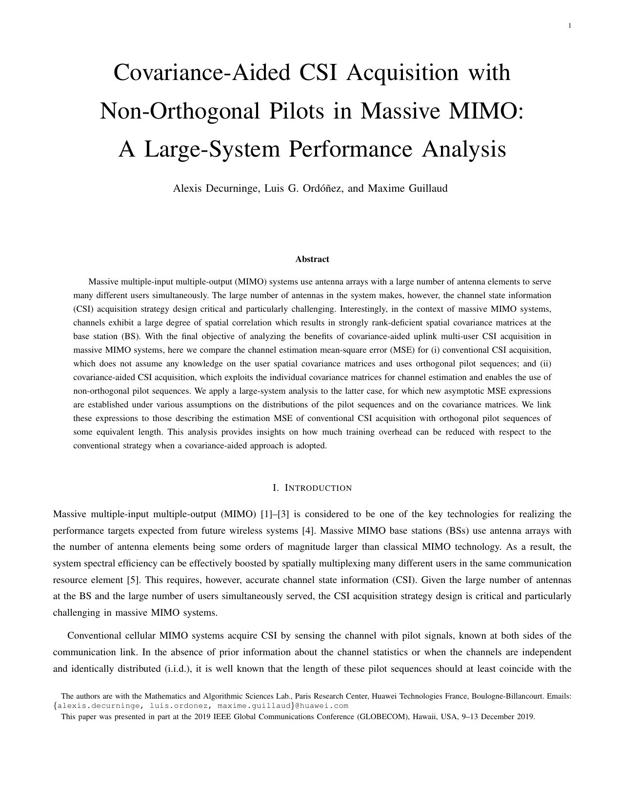 Figure 1
|
Deterministic Equivalent
to the estimation MSE |
Covariance
Matrices |
Pilots | Asymptotic Regime | |
|---|---|---|---|---|
| Thm. 1 |
deterministic
random |
deterministic |
with ratios , where
finite |
|
| Thm. 2 |
,
deterministic |
random |
finite
with ratio , where |
|
| Thm. 3 |
,
deterministic |
random |
with ratios:
with ratio , where , and there exists such that |
|
| Thm. 4 |
deterministic
random |
random |
with ratios:
, where , where , and there exists such that |
Peer Reviews
No public reviews on file for this paper yet. If you reviewed it on a platform where reviews are public (OpenReview, ICLR, NeurIPS, ICML), you can paste yours below so the community can read it here.
Videos
No videos yet. Explain this paper in a talk, walkthrough, or lecture? Add one.
Taxonomy
TopicsAdvanced MIMO Systems Optimization · Advanced Wireless Communication Techniques · Direction-of-Arrival Estimation Techniques
Covariance-Aided CSI Acquisition with Non-Orthogonal Pilots in Massive MIMO:
A Large-System Performance Analysis
Alexis Decurninge, Luis G. Ordóñez, and Maxime Guillaud The authors are with the Mathematics and Algorithmic Sciences Lab., Paris Research Center, Huawei Technologies France, Boulogne-Billancourt. Emails: {alexis.decurninge, luis.ordonez, maxime.guillaud}@huawei.comThis paper was presented in part at the 2019 IEEE Global Communications Conference (GLOBECOM), Hawaii, USA, 9–13 December 2019.
Abstract
Massive multiple-input multiple-output (MIMO) systems use antenna arrays with a large number of antenna elements to serve many different users simultaneously. The large number of antennas in the system makes, however, the channel state information (CSI) acquisition strategy design critical and particularly challenging. Interestingly, in the context of massive MIMO systems, channels exhibit a large degree of spatial correlation which results in strongly rank-deficient spatial covariance matrices at the base station (BS). With the final objective of analyzing the benefits of covariance-aided uplink multi-user CSI acquisition in massive MIMO systems, here we compare the channel estimation mean-square error (MSE) for (i) conventional CSI acquisition, which does not assume any knowledge on the user spatial covariance matrices and uses orthogonal pilot sequences; and (ii) covariance-aided CSI acquisition, which exploits the individual covariance matrices for channel estimation and enables the use of non-orthogonal pilot sequences. We apply a large-system analysis to the latter case, for which new asymptotic MSE expressions are established under various assumptions on the distributions of the pilot sequences and on the covariance matrices. We link these expressions to those describing the estimation MSE of conventional CSI acquisition with orthogonal pilot sequences of some equivalent length. This analysis provides insights on how much training overhead can be reduced with respect to the conventional strategy when a covariance-aided approach is adopted.
I Introduction
Massive multiple-input multiple-output (MIMO) [1, 2, 3] is considered to be one of the key technologies for realizing the performance targets expected from future wireless systems [4]. Massive MIMO base stations (BSs) use antenna arrays with the number of antenna elements being some orders of magnitude larger than classical MIMO technology. As a result, the system spectral efficiency can be effectively boosted by spatially multiplexing many different users in the same communication resource element [5]. This requires, however, accurate channel state information (CSI). Given the large number of antennas at the BS and the large number of users simultaneously served, the CSI acquisition strategy design is critical and particularly challenging in massive MIMO systems.
Conventional cellular MIMO systems acquire CSI by sensing the channel with pilot signals, known at both sides of the communication link. In the absence of prior information about the channel statistics or when the channels are independent and identically distributed (i.i.d.), it is well known that the length of these pilot sequences should at least coincide with the total number of transmit antennas in the system [6] for the channels to be identifiable. Additionally, mutually orthogonal pilot sequences are preferred, since they result in a better channel estimation accuracy with covariance-agnostic channel estimators [6, 7]. For the problem we consider in this paper, i.e., uplink (UL) CSI acquisition in a massive MIMO system serving single-antenna users, these conditions impose the pilot length to be at least equal to the number of users for which the channel is being simultaneously estimated. Depending on the coherence time of the channel or, more exactly, on the channel sensing periodicity, the transmission of long pilots sequences (to guarantee orthogonality) instead of data-bearing symbols can represent a significant loss in UL spectral efficiency.
Interestingly, in the context of massive MIMO systems, channels are far from being i.i.d and, in contrast, they exhibit a large degree of spatial correlation which results in a strongly rank-deficient spatial covariance matrix at the BS, as shown by numerous channel measurements campaigns as well as by theoretical channel models. For instance, experimental data in [8] show that the measured weakest channel singular values are significantly smaller than what would be expected under the Gaussian i.i.d. fading hypothesis [9]. This phenomenon is due to the fact that a small number of specular paths dominate in the propagation scenario, as put in evidence e.g. in [10]. Independent experimental results in [11] confirm a rank-deficient spatial covariance matrix by analyzing the channel correlation and channel matrix condition number observed with a cylindrical array of 112 elements in a mixed line-of-sight and non-line-of-sight scenario. Since the observed correlation is not mitigated by increasing the number of elements in the antenna array, we can conclude that it is a fundamental property of the propagation environment. Furthermore, this rank-deficient property holds irrespective of the massive MIMO array geometry: [8] uses a uniform linear array, [11] a cylindrical array, and [9] a 2D array for the covariance eigenvalue profile analysis. On a more theoretical side, it was shown in [12, 13] that if the support of the angle of arrival distribution is assumed to be bounded, the channel covariance matrix is rank-deficient with a rank depending on the tightness of the support bounds.
Consequently, by exploiting the rank-deficiency property, covariance-aided techniques are likely to be a key ingredient in the design of spectrally efficient massive MIMO systems. Indeed, [14] demonstrates that sharing (perfect) covariance information across different cells results in unbounded spectral efficiencies (as the number of BS antennas increases without bound) under a fairly mild assumption on the linear independence between the user covariance matrices. In the context of CSI acquisition, covariance information has been mainly exploited to propose orthogonal pilot reuse strategies[12, 13, 15, 16] or non-orthogonal pilot designs [17, 18, 19] to mitigate pilot contamination[20, 21, 22], that is, the undesired effect of obtaining a channel estimate that is contaminated by the channels of other users. All these methods rely on the intuition that users can be (partially) separated in space using their individual covariance matrices during the CSI acquisition process and perfectly orthogonal pilot sequences are no longer needed. In the extreme case of all the individual covariance matrices spanning mutually orthogonal subspaces, unit-length pilot sequences are sufficient to guarantee channel identifiability [17]. Unfortunately, it is difficult to know how spatial covariance information helps reducing the training overhead required by orthogonal pilots beyond this limit situation.
This work aims at analyzing the fundamental performance of covariance-aided CSI acquisition with non-orthogonal pilots in the massive MIMO regime, i.e., when the individual spatial covariance matrices are rank-deficient and possibly span non-orthogonal subspaces. With this objective, we focus on a MIMO system acquiring the CSI in the uplink under the assumption that the BS is able to perfectly track the individual spatial covariance matrices of all users with negligible additional pilot sequences (as described e.g. in [23]). We study analytically the channel estimation mean-square error (MSE) for the following cases: (i) conventional CSI acquisition, which does not assume any spatial covariance knowledge and uses orthogonal pilot sequences; and (ii) covariance-aided CSI acquisition, which exploits the individual spatial covariance matrices for channel estimation and possibly uses non-orthogonal pilot sequences. This work is motivated by the difficulty of interpreting the estimation MSE formulas for case (ii) under general covariance matrices and pilot sequences. Specifically, our contribution is as follows:
- •
We derive deterministic equivalents for the covariance-aided estimation MSE under different assumptions (either random or deterministic) for the covariance matrices and the set of pilot sequences. This allows to better understand a general situation beyond the extreme cases when orthogonal pilot sequences are used or when the individual spatial covariance matrices span mutually orthogonal subspaces.
- •
When the covariance matrices and the pilots sequences are assumed to be drawn from certain random distributions, we link the deterministic equivalent obtained for case (ii) to the MSE expression of case (i) with orthogonal pilots of an equivalent length depending on the received SNRs and the ranks of the covariance matrices of all the users in the system. This result is used to answer the question of how much the training overhead can be reduced with respect to orthogonal pilots when covariance-aided CSI acquisition is adopted and at least the performance of conventional CSI acquisition needs to be guaranteed.
- •
In order to obtain the deterministic equivalents for the MSE in the covariance-aided case, we derive new results on random matrix theory, which are of interest in their own. In particular, we extend the well-known trace-lemma, initially stated in [24], to block matrices in Proposition 3 using the so-called block-trace operator [25].
The rest of the paper is organized as follows. In Section II we introduce the channel model and describe in detail the adopted training-based CSI acquisition process. Section III presents the channel estimation MSEs for both the conventional and the covariance-aided CSI acquisition schemes, whereas Section IV contains the main contribution of this paper, that is, the large-system analysis of the covariance-aided MSE for different covariance matrices and non-orthogonal pilots models. Additionally we apply in Section IV the obtained deterministic equivalents to approximately solve the so-called CSI pilot length optimization problem in closed-form. Finally, in Section V we validate our results via numerical simulations.
II Preliminaries
In this paper we consider a massive MIMO system, in which a massive MIMO BS with antennas estimates the UL channels for single-antenna users using pilot sequences of length . The CSI acquisition process can be summarized as follows. First, the users simultaneously transmit their corresponding length- pilot sequences, which are not necessarily orthogonal, over the same communication resource elements (e.g., subcarriers in the case of orthogonal frequency-division multiplexing). Then, the BS collects the observations and estimates the UL channels for the users by means of a linear MMSE (LMMSE) channel estimator. In the following, we discuss the channel model and we describe the CSI acquisition procedure in more detail.
II-A Channel Model
Let us assume that the narrowband channel connecting the -th single-antenna user with the BS antennas, \mathbf{h}_{k}\in\mbox{\mathbb{C}}^{M}, can be expressed as
[TABLE]
where models the small-scale fading process, denotes the pathloss, and is the rank- spatial covariance matrix of user . Here we adopt the widely accepted “windowed” wide-sense stationary (WSS) fading channel model (see [13, 26, 27] for details), which assumes that the small scale fading coefficients in are drawn independently and kept fixed during the channel coherence time , whereas the slow time-varying large-scale fading parameters (second-order statistics), are considered to remain constant over a window . In consequence, the channel can be approximated as WSS inside this window and we can define
[TABLE]
where \mathbf{U}_{k}=(\mathbf{u}_{k,1},\ldots,\mathbf{u}_{k,r_{k}})\in\mbox{\mathbb{C}}^{M\times r_{k}} contains the eigenvectors associated with the non-zero eigenvalues of , , and \mathbf{\Lambda}_{k}=\mathrm{diag}\big{(}\lambda_{k,1},\ldots,\lambda_{k,r_{k}}\big{)}. Additionally, we normalize the covariance matrices to guarantee that
[TABLE]
II-B CSI Acquisition Model
The training-based CSI acquisition strategy can be described as follows. We denote by \mathbf{P}\in\mbox{\mathbb{C}}^{L\times(K+1)} the matrix gathering the length- pilot sequences assigned to the users:
[TABLE]
where \mathbf{p}_{k}=\big{(}p_{k}(1),\ldots,p_{k}(L)\big{)}^{\mathrm{T}} satisfies111Note that this power normalization is more realistic than the assumption that independently of commonly adopted in the pilot design literature.
[TABLE]
Letting all users simultaneously transmit their respective pilot sequence, the signal received by the BS at the -th resource element, \mathbf{y}(\ell)\in\mbox{\mathbb{C}}^{M}, is
[TABLE]
where are the transmit powers and \mathbf{n}(\ell)=\big{(}n_{1}(\ell),\ldots,n_{M}(\ell)\big{)}^{\mathrm{T}}\in\mathbb{C}^{M} denotes the additive white Gaussian noise with i.i.d. circularly symmetric components, for . Grouping the received signal for the resource elements dedicated to training in \mathbf{Y}=\big{(}\mathbf{y}(1),\ldots,\mathbf{y}(L)\big{)}\in\mbox{\mathbb{C}}^{M\times L}, the signal model in (6) can be more compactly expressed as
[TABLE]
with \mathbf{H}=\big{(}\mathbf{h}_{0},\cdots,\mathbf{h}_{K}\big{)}\in\mbox{\mathbb{C}}^{M\times(K+1)}, \mathbf{D}_{\boldsymbol{P}}=\mathrm{diag}\big{(}P_{0},\ldots,P_{K}\big{)}\in\mbox{\mathbb{R}}_{+}^{(K+1)\times(K+1)}, and \mathbf{N}=\big{(}\mathbf{n}(1),\cdots,\mathbf{n}(L)\big{)}\in\mbox{\mathbb{C}}^{M\times L}. We can equivalently write
[TABLE]
where we have defined \mathbf{h}=\mathrm{vec}(\mathbf{H})=\big{(}\mathbf{h}_{0}^{\mathrm{T}},\ldots,\mathbf{h}_{K}^{\mathrm{T}}\big{)}^{\mathrm{T}}, , and .
Given the observation model in (8), the BS estimates the individual channels from the users, adopting a LMMSE approach, which under the channel model in (1) is given by [28, Chap. 12]
[TABLE]
where we have introduced the received signal-to-noise ratios (SNRs), , , and \mathbf{\Sigma}=\mathrm{diag}\big{(}\mathbf{\Sigma}_{0},\ldots,\mathbf{\Sigma}_{K}\big{)}. Observe that the estimator in (9) requires the knowledge of the second-order statistics of the individual channels. When this information is not available, the estimator in (9) is substituted by a mismatched estimator, which has different accuracy depending on how much is assumed to be known from the channel model in (1). In particular, we distinguish between the following cases:
- (i)
Conventional CSI Acquisition Strategy: We assume that the BS either does not have or does not use the individual spatial covariance matrices and, hence, uses . It knows the transmit powers , and the received signal-to-noise ratios (SNRs) including the pathloss information. We also consider that the pilot set gathered in is orthogonal, i.e.,
[TABLE]
which requires the pilot-length to satisfy . Then, the channel estimator in (9) becomes the mismatched LMMSE estimator \hat{\mathbf{h}}^{\mathsf{(i)}}=\big{(}(\mathbf{h}^{\mathsf{(i)}}_{0})^{\mathrm{T}},\ldots,(\mathbf{h}^{\mathsf{(i)}}_{K})^{\mathrm{T}}\big{)}^{\mathrm{T}} with given by
[TABLE]
where . This channel estimation technique coincides with the element-wise MMSE estimator in [3, Sec. 3.4] when the diagonal entries of the individual spatial covariance matrices are assumed to be 1. This case is analyzed in Section III-A.
- (ii)
Covariance-Aided CSI Acquisition Strategy: We assume that the BS exploits the knowledge of the individual spatial covariance matrices , the transmit powers , and the received SNRs , during CSI acquisition, and uses an arbitrary (possibly non-orthogonal) pilot set , i.e., (10) is not satisfied. The channel estimator in that case is directly obtained from (9), that is, \hat{\mathbf{h}}^{\mathsf{(ii)}}=\big{(}(\mathbf{h}^{\mathsf{(ii)}}_{0})^{\mathrm{T}},\ldots,(\mathbf{h}^{\mathsf{(ii)}}_{K})^{\mathrm{T}}\big{)}^{\mathrm{T}} with given by
[TABLE]
This case is investigated in Sections III-B and IV.
II-C CSI identifiability
Let us now present the identifiability conditions on the system parameters: the pilot length and the ranks of the individual covariance matrices , which enable to identify the CSI vector from the observations in (8) in the noiseless case (). Using an equation counting argument, we see that CSI identifiability requires or, equivalently, that
[TABLE]
where , so that the system can be uniquely inverted. Since has rows and columns, a necessary condition for CSI identifiability is
[TABLE]
In particular, if all covariance matrices are full rank, , the CSI is identifiable if and only if , i.e., it is necessary that . On the contrary, if all the covariance matrices span orthogonal subspaces, we necessarily have that and, hence, the CSI is identifiable for . Besides these two extreme cases, it is hard to establish identifiability conditions for general pilot sequences and user covariance matrices and this is exactly what complicates the MSE analysis of covariance-aided CSI acquisition. Still, thanks to the large-system analysis in Section IV, we are able extract meaningful conclusions for the intermediate cases.
III MSE Analysis of CSI Acquisition Strategies
In this section we present the channel estimation MSE expressions for both the conventional and the covariance-aided CSI acquisition schemes. In particular, we characterize the performance of each CSI acquisition strategy by the channel estimation mean-square error (MSE) of a given user, denoted as user [math]. This incurs in no loss of generality and allows us to derive useful insights by considering the other users as interferers.
III-A Conventional CSI Acquisition
Let us first focus on the conventional CSI acquisition strategy, which uses orthogonal pilots and applies the mismatched (covariance-agnostic) LMMSE channel estimator in (11). The channel estimation error covariance matrix in this case is given by
[TABLE]
with , and the individual error covariance matrix for user [math] follows from the first block of in the diagonal of \mathbf{C}_{\mathbf{e}}^{(\mathsf{i})}\big{(}\{\mathbf{\Sigma}_{k}\},\{\mathsf{snr}_{k}\}\big{)}:
[TABLE]
The channel estimation MSE for user [math] can be derived from (16) as presented in the next lemma.
Lemma 1**.**
Let the pilot set contain orthogonal pilot sequences of length , so that (10) holds. Then, the individual MSE of estimating with the estimator in (11) is given by
[TABLE]
III-B Covariance-Aided CSI Acquisition
Let us now analyze the case in which the spatial covariance matrices are exploited in the CSI acquisition process. In consequence, let us assume now that the BS knows the spatial covariance matrices , the transmit powers , and the received SNRs, , and estimates the channel using the LMMSE estimator in (12). Then, the channel estimation error covariance matrix is given by
[TABLE]
and, hence, the individual error covariance matrix for user [math] is
[TABLE]
Finally, the channel estimation MSE for user [math] in the covariance-aided case is
[TABLE]
where we have used the covariance matrix decomposition in (2) and Lemma 3 postponed in Appendix A.
For convenience, let us now introduce the estimation signal-to-interference-plus-noise ratio (SINR) as follows. Recall from (12) that with \mathbf{E}_{0}\triangleq\big{(}\mathsf{snr}_{0}/\sqrt{P_{0}}\big{)}\big{(}\tilde{\mathbf{P}}\tilde{\mathbf{D}}_{\mathsf{snr}}^{1/2}\mathbf{\Sigma}\tilde{\mathbf{D}}_{\mathsf{snr}}^{1/2}\tilde{\mathbf{P}}^{\dagger}+\mathbf{I}_{LM}\big{)}^{-1}\tilde{\mathbf{P}}_{0}\mathbf{\Sigma}_{0} and the received signal as given in (8). Thanks to the linearity of the estimator, we can identify the useful signal as the contribution originated from the transmission of by user [math], i.e., and denote the rest as interference-plus-noise, i.e., \mathbf{E}_{0}^{\dagger}\big{(}\mathbf{y}-\sqrt{P_{0}}\mathbf{E}_{0}^{\dagger}\tilde{\mathbf{P}}_{0}\mathbf{h}_{0}\big{)}. Accordingly, we define the estimation SINR measured in the subspace spanned by each eigenvector of as the ratio of the expectation (with respect to the noise) of the two quantities, i.e.,
[TABLE]
where we used again Lemma 3. Identifying terms, we can now rewrite the MSE expression in (22) as
[TABLE]
It is interesting to observe (e.g., in (23)) that \mathsf{sinr}_{0,i}^{(\mathsf{ii})}\big{(}\mathbf{P},\{\mathbf{\Sigma}_{k}\},\{\mathsf{snr}_{k}\}\big{)}\leq L\mathsf{snr}_{0}\lambda_{0,i}, where the upper bound is achieved for , when the interference from the users is completely canceled by LMMSE channel estimator. In that case the MSE in the following lemma results.
Lemma 2**.**
Let one or both following conditions hold:
- (a)
(Orthogonal pilot condition). Pilot sequence is orthogonal to the rest of pilot sequences, i.e.,
[TABLE]
- (b)
(Orthogonal covariance subspaces). The -dimensional subspace spanned by the covariance matrix of user [math] is orthogonal to the subspace spanned by the covariance matrices of the interfering users, i.e.,
[TABLE]
Then, \mathsf{sinr}_{0,i}^{(\mathsf{ii})}\big{(}\mathbf{P},\{\mathbf{\Sigma}_{k}\},\{\mathsf{snr}_{k}\}\big{)}=L\mathsf{snr}_{0}\lambda_{0,i} and the individual MSE of estimating with the estimator in (12) is
[TABLE]
where are the non-zero eigenvalues of as introduced in (2).
Observing that is concave in for any , we can apply Jensen’s inequality to see that
[TABLE]
with equality when . We can conclude that, under the conditions of Lemma 2, covariance-aided CSI acquisition strictly outperforms the conventional strategy with orthogonal pilots in a massive MIMO system, that is, \mathsf{mse}^{(\mathsf{ii})}_{0}\big{(}\mathbf{\Sigma}_{0},\mathsf{snr}_{0}\big{)}<\mathsf{mse}^{(\mathsf{i})}_{0}\big{(}\mathsf{snr}_{0}\big{)}, whenever the eigenvalues are not all equal and, in particular, when the spatial covariance matrix of user [math] is not full-rank (). This can be easily interpreted as follows. Both the conventional and the covariance-aided CSI strategies under the conditions in Lemma 2 effectively remove any interference caused by the pilots of the remaining users, so that they become purely noise-limited. The covariance-aided channel estimator in (12) additionally removes all the noise outside the subspace spanned by and this reduces the noise power at least by a factor of , as confirmed by (29).
IV Large-System Analysis of Covariance-Aided CSI Acquisition
Given the difficulty of interpreting the effect of the pilot sequences and the spatial covariance matrices on the channel estimation MSE for the covariance-aided CSI acquisition strategy as given in (22), in this section we adopt a large-scale analysis approach. Indeed, we study \mathsf{mse}^{(\mathsf{ii})}_{0}\big{(}\mathbf{P},\{\mathbf{\Sigma}_{k}\},\{\mathsf{snr}_{k}\}\big{)} asymptotically in with given fixed ratios under different assumptions on and \mathbf{P}\in\mbox{\mathbb{C}}^{L\times(K+1)} and derive the corresponding deterministic equivalents as summarized in Table 3. Deterministic equivalents provide asymptotically tight deterministic approximations for the MSE, which allow us to decouple the effects of the non-orthogonality of the pilots and the non-orthogonality of the covariance matrices.
IV-A Deterministic Equivalent for Random Covariance Matrices and Deterministic Pilots
Let us assume in this section that the pilot length and the number of interfering users are finite and that the individual covariance matrix of user [math], , and the pilots sequences are deterministic. Furthermore, the individual spatial covariance matrices of the interfering users are assumed to be drawn from a random distribution.
Besides the rank-deficiency, little information is available about the distribution of realistic spatial covariance matrices in massive MIMO, as few experimental works have concentrated specifically on that point (it would require to measure the channel with different array geometries and over different scenarios). Therefore, we adopt the maximum entropy principle [29], and observe that among all the distributions over rank- positive semidefinite matrices of a given size and trace, the Wishart distribution with degrees of freedom and column covariance matrix proportional to the identity is the one that has maximum differential entropy [30, Section 18.2.2.3]. Accordingly, we assume the following (general) random model for the individual spatial covariance matrices.
Assumption A1** (Random covariance model).**
The individual covariance matrices of the interfering users are assumed to be random according to:
[TABLE]
where is the rank of with probability and the entries of are i.i.d. with zero-mean, unit variance, and have finite eighth order moment. Observe that the covariance matrix normalization in (3) is now satisfied in expectation.
Note that Assumption A1 is in fact more general than the maximum entropy covariance matrix assumption. The (entropy maximizing) Wishart distribution is obtained by adding the Gaussianity assumption to A1.
Then, the deterministic equivalent of the MSE of user [math] as given in the next theorem follows.
Theorem 1**.**
Assume that the individual covariance matrices of the interfering users, , follow Assumption A1. Let denote the non-zero eigenvalues of and define
[TABLE]
where
[TABLE]
and the constants are given by the unique nonnegative solutions to the following fixed point equations:
[TABLE]
Then, as and grow large with ratios such that , we have that
[TABLE]
Proof. The proof is mainly based on an application of [31, Thm. 1]. See Appendix B-A.
The result in Theorem 1 is useful to see the effect of using non-orthogonal pilots on the CSI acquisition accuracy. Note that the constant measures the level of interference created by the pilot sequence of user when estimating the channel of user [math] (the larger , the lower the interference). In particular, if the pilots are orthogonal (see condition (a) in Lemma 2), it holds that and the deterministic equivalent in (31) becomes the MSE given in Lemma 2 for the interference-free case.
IV-B Deterministic Equivalent for Deterministic Covariance Matrices and Random Pilots
Let us now assume that all the covariance matrices are deterministic and consider the following random model for the pilot sequences.
Assumption A2** (Random pilot model).**
The random length- pilot sequences are of the form
[TABLE]
with \mathbf{p}_{0},\ldots,\mathbf{p}_{K}\in\mbox{\mathbb{C}}^{L} being independent random vectors with i.i.d. entries of zero-mean, unit variance, and have finite eighth order moment. Observe that the normalization in (5) is now satisfied in expectation.
Furthermore, we assume that the pilot length is sufficient to estimate the subspace spanned by the covariance matrices of all users as formalized next.
Assumption A3** (Pilot length).**
There exists such that
[TABLE]
with \mathbf{U}_{k}\in\mbox{\mathbb{C}}^{M\times r_{k}} containing the eigenvectors associated with the non-zero eigenvalues of .
Indeed, Assumption A3 is related to the system identifiability discussed in Section II-C. If (36) holds, one immediate consequence is that
[TABLE]
which is a necessary condition for asymptotic identifiability (see (14)).
For convenience, let us introduce the block version of the trace operator for block matrices (see [25] for details) before presenting the deterministic equivalent of the MSE error of user [math] as in the next theorem.
Definition 1**.**
Consider a matrix composed of blocks of size , i.e.
[TABLE]
The block-trace of is defined as444Note that this definition is highly dependent on the size of the blocks . We omit, however, the reference to in the notation for the sake of simplicity.
[TABLE]
Theorem 2**.**
Assume that all pilot sequences are random pilots satisfying Assumption A2 and the pilot-length is such that Assumption A3 holds. Let denote the non-zero eigenvalues of and the corresponding eigenvectors and define
[TABLE]
where is the unique positive definite matrix solution to the following fixed point equation
[TABLE]
where the block-trace operator is introduced in Definition 1. Then, as and grow large with ratio such that and whenever there exists such that
[TABLE]
we have that
[TABLE]
Proof. The idea of the proof is to generalize the result of Bai and Silverstein [32] to block-matrices in order to provide a deterministic equivalent for . The main step consists in using the equivalent of a rank-1 perturbation for block matrices and proving that the fixed point mapping underlying (41) is satisfied by and that it is indeed a contraction. As a key ingredient, we generalize the trace lemma to block-matrices with convenient random matrix concentration inequalities in Proposition 3 of Appendix A. See the detailed proof of Theorem 2 in Appendix B-B.
The result in Theorem 2 is useful to understand the effect of the relative orthogonality between the subspace spanned by the covariance matrix of user 0, , and the subspace spanned by the covariance matrices of the interfering users, as captured by the estimation SINR term in (40). In particular, when the subspace spanned by the covariance matrix of user [math] is orthogonal to the subspace spanned by the other users, i.e., \mathbf{u}_{0,i}^{\dagger}\Big{(}\sum_{k=1}^{K}\mathbf{U}_{k}\mathbf{U}_{k}^{\dagger}\Big{)}\mathbf{u}_{0,i}=0 for (see condition (b) in Lemma 2), it follows from (41) that the deterministic equivalent in (40) becomes the MSE given in Lemma 2. The reason is that the projection into the subspace of user [math] in the channel estimator in (12) already cancels all interference from the other users and orthogonal pilots are no longer needed. Moreover, using the fixed point equation in (41), the SINR can be upper bounded using the inequality
[TABLE]
where in (45) we use that and that ,555Let be Hermitian matrices. We say that , if is positive semidefinite. and (46) follows from using the Taylor expansion of \big{(}\frac{1}{L}\sum_{k=1}^{K}\mathbf{U}_{k}\mathbf{U}_{k}^{\dagger}+\mathbf{I}_{M}\big{)}^{-1} under the assumption in (36). Therefore, the larger the projection of on the interferer covariance matrix, the lower the SINR.
In order to extend the results of Theorem 2 for the case , we need to ensure that the convergence in (44) holds uniformly in . This is done in the following theorem.
Theorem 3**.**
Assume that all pilot sequences are random pilots satisfying Assumption A2 and the pilot-length is such that Assumption A3 holds uniformly in . Assume that pilot is uniformly bounded, i.e., there exists such that for any it holds a.s.666This assumption is always satisfied in practice, since the maximum transmit power is always limited. If, furthermore, in (43) is independent from and there exists such that , the convergence of \mathsf{mse}_{0}^{(\mathsf{ii})}\big{(}\mathbf{P},\{\mathbf{\Sigma}_{k}\},\{\mathsf{snr}_{k}\}\big{)} to the deterministic equivalent \xi_{0}^{(\mathsf{ii})}\big{(}\{\mathbf{\Sigma}_{k}\},\{\mathsf{snr}_{k}\};\mathbf{\Gamma}_{L}\big{)} introduced in Theorem 2 is uniform in .
Proof. See Appendix B-C.
Finally, recall that the deterministic equivalent in Theorems 2 (and 3) only holds under some technical condition given in (43) on matrix defined in (42). For completeness we provide in the following proposition two alternative sufficient conditions on the system parameters for guaranteeing the required result.
Proposition 1**.**
Let be defined as in (42), and let the pilot sequence satisfy Assumption A2. Then, there exists such that a.s., whenever one of the following conditions hold:
- (a)
(Summable received SNRs condition). The covariance matrices have uniformly bounded spectral norm and
[TABLE]
- (b)
(Strong subspace identifiability condition). There exists a constant such that
[TABLE]
where \mathbf{U}=\mathrm{diag}\big{(}\mathbf{U}_{0},\mathbf{U}_{1},\dots,\mathbf{U}_{K}\big{)}\in\mbox{\mathbb{C}}^{(K+1)M\times\sum_{k=0}^{K}r_{k}} gathers the eigenvectors of the individual covariance matrices of the users as defined in (2).
Moreover, if (a) holds or if in (b) is independent of , then is also independent of .
Proof. See Appendix B-D.
Observe that the conditions in (a) imply that the power of the interference perceived by user [math] from the other users (which is proportional to ) decreases fast enough, so that the interference level is controlled independently of the particular covariance eigenspaces. Alternatively, condition (b) ensures, without imposing any restriction on the power of the interfering users, that random pilots are good enough for CSI acquisition given the relative orthogonality between the covariance eigenspaces of all users in the system. In fact, (48) is slightly stronger than the channel identifiability condition, which consists in assuming that (see Section II-C). Note that if , [24, Thm. 1.1] guarantees the existence of some constant such that a.s., so that condition (b) in (48) is satisfied in that case.
IV-C Deterministic Equivalent for Random Covariance Matrices and Random Pilots
Let us now focus on the case in which the covariance matrices follow the random model in Assumption A1 and the pilot sequences follow the random model in Assumption A2. To this end, we particularize the results in Section IV-B for random covariance matrices. In the following proposition we give a deterministic equivalent in Frobenius norm for the fixed point matrix in Theorem 2 when .
Proposition 2**.**
Assume that the individual covariance matrices of the interfering users satisfy Assumption A1. Let be the solution of the fixed point equation in (41) and be the unique solution to the following the fixed point equation
[TABLE]
Further assume that Assumption A3 holds uniformly in and define and . Then, as and grow large with ratio , and and grow large with ratios satisfying for , it holds that
[TABLE]
Then, when and , we have that
[TABLE]
Proof. See Appendix B-E.
We are now in the position to present in the next theorem the deterministic equivalent for the MSE of user [math] when the individual covariance matrices of the interfering users and all the pilot sequences are random and as , and grow large with some fixed ratios.
Theorem 4**.**
Assume that the individual covariance matrices of the interfering users satisfy Assumption A1 and that all length- pilot sequences are random pilots satisfying Assumption A2. Let denote the non-zero eigenvalues of and define
[TABLE]
with being the unique solution to the fixed point equation in (49). Then, under the conditions of Theorem 3 and in the asymptotic regime of Proposition 2, we have that
[TABLE]
Proof. See Appendix B-F.
Observe that the deterministic equivalent for the MSE of user [math] in (52) has a very similar expression to the MSE given in Lemma 2. More precisely, the LMMSE estimator with non-orthogonal pilots of length in the large-system regime becomes equivalent to the LMMSE estimator with orthogonal pilots of length see Lemma , where is the solution of (49). Thus, the effect of pilot contamination can be understood as an effective reduction of the estimation SINRs (see definition in (24)) from to , where satisfies the bounds in (50), or, following the discussion in [3, Sec. 3.2] as an effective reduction of the pilot processing gain. Accordingly, we can define the equivalent pilot processing gain/length of random non-orthogonal pilots as .
It is very interesting to investigate under which conditions on the system parameters, more exactly, on the received SNRs and the covariance ranks of the interfering users, these limiting values are attained.
Corollary 1**.**
Define
[TABLE]
Then, under the conditions of Theorem 4, it holds that
[TABLE]
where constant takes the following values:
- (a)
, whenever
[TABLE]
- (b)
* with , whenever*
[TABLE]
Proof. See Appendix B-G.
The conditions in Corollary 1 can be interpreted as sufficient conditions for the system to be either (a) interference-free or (b) pilot-contaminated. Recall that the SNR of user is defined as , where denotes the pathloss. As an example, let us consider that the cell size increases with the number of users and that the users are uniformly distributed over the cell. Then, under a suitable ordering of the users according to the pathloss, there exists some constants and such that , and the conditions in Corollary 1.(a) are satisfied. Hence, we are in the noise-limited scenario and the deterministic equivalent in (52) takes the form of the MSE expression in Lemma 2 for the interference-free case. To the contrary, when the cell size is fixed and the users are uniformly distributed in the cell, there exists some constant such that for . Thus, the conditions in Corollary 1.(b) are fulfilled and the LMMSE estimator does not completely remove interference. In that case, the estimation SINRs gets reduced by a factor of due to the effect of pilot contamination.
IV-D Covariance-Aided CSI Acquisition for Training Overhead Reduction
Let us now illustrate how the previous large-system analysis can be used to quantify the benefits of exploiting the knowledge of the user covariance matrices during CSI acquisition in order to reduce the training overhead beyond the extreme cases of mutually orthogonal pilots and/or covariance matrices. This can be more formally stated as follows.
Problem Formulation** (Pilot length optimization).**
Given a massive MIMO system with BS antennas serving users, we seek the minimum pilot length which guarantees for the covariance-aided CSI acquisition in (12) (case (ii)) at least the same average channel estimation performance obtained by the conventional CSI acquisition scheme in (11) with orthogonal pilots (case (i)) of length , that is, the minimum pilot length such that
[TABLE]
where and \mathsf{mse}_{0}^{\mathsf{(ii)}}\big{(}\mathbf{P},\{\mathbf{\Sigma}_{k}\},\{\mathsf{snr}_{k}\}\big{)} are defined in (17) and (22), respectively.
The previous pilot length optimization problem is difficult to solve based on the MSE expression depending of the exact covariance matrices and pilots given in (22). However, it can be approximated in closed form using the deterministic equivalent in Corollary 1.(b) as follows. We upper-bound the deterministic equivalent using Jensen’s inequality as in (29):
[TABLE]
so that the performance guarantee condition in (58) can be simply approximated in the large-system limit as
[TABLE]
which implies that can be approximated by given by
[TABLE]
The length in (61) can be interpreted as follows. The first term, , corresponds to the noise reduction obtained from the projection into the -dimensional subspace spanned by the covariance matrix of user [math] performed by the covariance-aided channel estimator in (12). The second term, , accounts for the loss due the interference of the other users as it is explicit in (22). The result suggests moreover that non-orthogonal pilots are useful only if
[TABLE]
Indeed, if it is not the case, the approximated minimum length is necessarily greater than , meaning that the use of orthogonal pilots will result in better channel estimation accuracy even if the individual covariance matrices are exploited. This can be explained by the fact that orthogonal pilots naturally completely remove interference between users while the interference induced by non-orthogonal pilots cannot be not compensated by the covariance matrix knowledge if (62) does not hold.
To the contrary, whenever (62) is satisfied, covariance-aided CSI acquisition allows to reduce the pilot length with respect to conventional CSI acquisition with orthogonal pilots of length by a factor . This ratio can be approximated by satisfying
[TABLE]
The accuracy of the approximation of by and that of by is numerically investigated in Section V.
V Numerical Evaluation
In this section we illustrate numerically the accuracy of the deterministic equivalents presented in Theorems 1-4 and Corollary 1. For doing so, we consider the following the random pilots and covariance matrix models.
Non-Orthogonal Pilots Model**.**
Given the number of users , we generate the pilot sequences \mathbf{p}_{k}=\big{(}p_{k}(1),\ldots,p_{k}(L)\big{)}^{\mathrm{T}} of length for as
[TABLE]
where are i.i.d. random variables uniformly distributed in (this model satisfies Assumption A2) and we generate the covariance matrices using one of the following models.
Covariance Matrix Model 1** (Maximum Entropy).**
Under the maximum entropy principle, the individual spatial covariance matrices are modeled as
[TABLE]
where denotes the rank, the entries of \mathbf{X}_{k}\in\mbox{\mathbb{C}}^{M\times r_{k}} are i.i.d. complex Gaussian zero-mean, unit variance random variables. This model satisfies Assumption A1.
Alternatively, we also consider a one-ring correlation model [13],[3, Sec. 2.6], which assumes that a user located at azimuth angle is surrounded by a cluster of scatterers creating multipath components with angles of arrival uniformly distributed in , where denotes the angular spread. In particular we generate the random spatial covariance matrices as follows.
Covariance Matrix Model 2** (One-Ring with UCA).**
Assume that the BS is equipped with uniform circular array (UCA) with antenna elements with half-wavelength spacing [33]. Under the one-ring model, the individual spatial covariance matrices are obtained as
[TABLE]
where , the azimuth angle is uniformly distributed in , the angular spread is set to .
Observe that this model does not satisfy Assumptions A1 since the ranks are random and cannot be explicitly controlled. We illustrate the difference by plotting the respective average normalized rank versus for both models in Figure 1.
First, in Figure 2a we plot the exact MSE for the covariance-aided CSI acquisition strategy (computed using (22)) and the approximations obtained from the deterministic equivalents in Theorems 1, 2, and 4 averaged over 100 realizations of the random pilots and covariance matrices. For each value of the BS antenna number , we set the number of users to , with , we generate the individual covariance matrices according to the maximum entropy model in (65) with and pathloss , and we allocate pilots of length following the model in (64). All the obtained deterministic equivalents provide a very good accuracy in approximating the actual MSE and this accuracy increases with the number of antennas as expected. This observation is further confirmed in Figure 2b, where we plot the normalized approximation error incurred by the different deterministic equivalents in order to measure the convergence of the approximation in the large-system limit and defined as
[TABLE]
where denotes the considered deterministic equivalent.
In this simulation setup, the effect of using non-orthogonal pilots is more important in the CSI estimation MSE than the relative orthogonality of the user covariance matrices. Indeed, we observe a higher accuracy achieved by the deterministic equivalent from Theorem 1, where the pilots are assumed to be deterministic and, hence, the actual pilot set is used to compute \xi_{0}^{(\mathsf{ii})}\big{(}\mathbf{P},\mathbf{\Sigma}_{0},\{\mathsf{snr}_{k}\}\big{)}. Furthermore, when the pilots are assumed to be random as done in Theorems 2 and 4, there is no appreciable accuracy improvement from using the exact covariance matrices (as in Theorem 2) with respect to modeling them as random (as in Theorem 4). In both figures, we have omitted the deterministic equivalent in Corollary 1, since under case (b) , it provides the same result as using the fixed point equation for in Proposition 2.
Let us now consider the one-ring correlation model with a BS equipped with a UCA as defined in Covariance Matrix Model 2 with unit pathloss for all users. For each covariance matrix, we compute its rank by using the Matlab function, defining then the rank as the number of eigenvalues whose ratio with the strongest eigenvalue is above the numerical precision (see Figure 1). We repeat the previous simulations and plot the results in Figure 3. Conversely to the maximum entropy model, the one-ring UCA covariance matrix model does not satisfy Assumption A1 and, hence, Theorems 1 and 4 do not hold in this case. Still, we can see in Figure 3 that the corresponding deterministic equivalents provide a fairly good approximation of the actual MSE but, as expected, Theorem 2 results in a higher accuracy, since it explicitly takes into account all individual covariance matrices.
Finally, in order to quantify the benefits of exploiting the knowledge of the user covariance matrices during CSI acquisition, we focus on the CSI training overhead reduction problem stated in Section IV-D. For each value of the BS antenna number , we set the number of users to , with , and we compute (using exhaustive search) the minimum pilot length required by covariance-aided CSI acquisition using random non-orthogonal pilots following the model in (64), which guarantees the same MSE as the conventional CSI acquisition strategy with orthogonal pilots of length . In Figures 4.(a) and 5.(a) we compare with the approximated minimum length L^{\mathsf{(ii)}}=\big{\lceil}(K+1)\tau_{M,0}+K\bar{\tau}_{M}\big{\rceil} for both the maximum entropy model with and for the one-ring UCA model with an angular spread of , respectively, averaged over 100 random realizations of the pilots and the covariance matrices. In both cases gives a very accurate approximation of \mathrm{E}\big{\{}L^{\star}\big{\}} which improves with increasing number of BS antennas. This is further confirmed in Figures 4.(b) and 5.(b), where we plot the average pilot reduction with respect to orthogonal pilots, defined as \Delta=L^{\mathsf{(i)}}/\mathrm{E}\big{\{}L\big{\}}=(K+1)/\mathrm{E}\big{\{}L\big{\}}, where either denotes or . In the case of maximum entropy covariance matrices, for which we can explicitly control the rank so that , we also include the large-system pilot-length reduction in (63), . This confirms the benefits of using covariance-aided CSI acquisition for significantly reducing the training overhead in massive MIMO systems.
VI Conclusions
We have applied a large-system analysis to characterize the performance of covariance-aided multi-user CSI estimation in the uplink of a massive MIMO system. Deterministic equivalents of the achieved estimation MSE were obtained under several assumptions related to the stochastic nature of the spatial covariance matrices and/or the pilot sequences. When the covariance matrices and the pilots sequences are assumed to be drawn from some i.i.d. random distributions, our results indicate that the performance of covariance-aided CSI acquisition can be interpreted as that of a system using orthogonal pilot sequences of certain equivalent pilot length, for which a closed-form expression enables an intuitive interpretation of the achieved MSE. Numerical results demonstrate that the covariance-based strategy allows to significantly reduce the training overhead with respect to conventional CSI acquisition. Finally, we contributed to random matrix analysis by extending the trace-lemma from [24] to block matrices.
Appendix A Preliminary Results
Lemma 3** (Woodbury identity).**
Let be respectively , , and complex matrices such that are invertible. Then
[TABLE]
Consider also \mathbf{x}\in\mbox{\mathbb{C}}^{N}, c\in\mbox{\mathbb{C}} for which is invertible. Then,
[TABLE]
Lemma 4** (Resolvent identity).**
Let and be two invertible complex matrices of size . Then,
[TABLE]
Lemma 5** ([24]).**
Let with \mathbf{A}_{N}\in\mbox{\mathbb{C}}^{N\times N} be a series of random matrices with uniformly bounded spectral norm on . Let with \mathbf{x}_{N}\in\mbox{\mathbb{C}}^{N}, be random vectors of i.i.d. entries with zero mean, unit variance, and finite eighth order moment, independent of . Then,
[TABLE]
Lemma 6** ([24, Lem. 2.7]).**
Under the conditions of Lemma 5, if for all and , \mathrm{E}\big{\{}|x_{M,k}|^{m}\big{\}}\leq\nu_{m}, then for all ,
[TABLE]
for some constant depending only on .
Lemma 7** ([30, Thm. 3.7]).**
Let with \mathbf{A}_{N}\in\mbox{\mathbb{C}}^{N\times N} be a series of random matrices with uniformly bounded spectral norm on . Let and , \mathbf{x}_{N}\in\mbox{\mathbb{C}}^{N} and \mathbf{y}_{N}\in\mbox{\mathbb{C}}^{N}, two series of random vectors with i.i.d. entries such that have zero mean, unit variance, and finite fourth order moment, independent of . Then,
[TABLE]
Lemma 8**.**
Let be two Hermitian matrices such that is positive semidefinite. Then,
[TABLE]
Proof.
Let denote the eigenvalues of and the corresponding eigenvectors. Then,
[TABLE]
where the last inequality holds since is positive semidefinite. ∎
Lemma 9**.**
Let be three series of matrices of size , and , respectively. Then, for
[TABLE]
and
[TABLE]
Proof.
Define matrices , of size , and the block diagonal matrix of size . Then, using Cauchy-Schwarz inequality, it holds
[TABLE]
Additionally, we prove the second part using Lemma 8
[TABLE]
∎
Let us now provide a blockified version generalizing the convergence of the trace lemma (see Lemma 5) for block-matrices with a convergence in spectral norm on blocks.
Proposition 3**.**
Let with \mathbf{A}^{(i,j)}_{M}\in\mbox{\mathbb{C}}^{M\times M} and \mathbf{A}^{(i,j)}_{M}=\big{(}\mathbf{A}^{(j,i)}_{M}\big{)}^{\dagger}, for , be a series of matrices. Let with \mathbf{A}_{M,L}\in\mbox{\mathbb{C}}^{ML\times ML} be a series of Hermitian matrices with uniformly bounded spectral norm gathering the blocks as
[TABLE]
Let with \mathbf{x}_{L}\in\mbox{\mathbb{C}}^{L}, be random vectors of i.i.d. entries with zero mean, variance , and finite eighth order moment, independent of , and let . Then, considering the block-trace operator defined in (1),
[TABLE]
Assume furthermore that the entries of \mathbf{x}_{L}=\big{(}x_{1},\ldots,x_{L}\big{)}^{\mathrm{T}} are bounded almost surely, i.e., there exists such that a.s. for . Then, if for some , it holds that
[TABLE]
Proof.
We divide the proof in two parts using different concentration inequalities. First, we prove (i) the non-uniform convergence result in (84) and, then, (ii) the uniform convergence in so that (85) holds.
Proof of (i).
Similarly to the proof of the trace lemma in [24], we need to find an integer such that
[TABLE]
where is a constant independent of , such that . Let us first introduce the matrix \mathbf{\Delta}_{M}=\frac{1}{L}\big{(}\mathbf{X}_{M,L}^{\dagger}\mathbf{A}_{M,L}\mathbf{X}_{M,L}-\mathrm{blktr}[\mathbf{A}_{M,L}]\big{)} with elements given by
[TABLE]
which can be rewritten as
[TABLE]
by introducing the matrices with elements given by \big{[}\bar{\mathbf{A}}_{L}^{(n,m)}]_{i,j}=[\mathbf{A}_{M}^{(i,j)}]_{n,m}. Then, from Lemma 6, we know that for ,
[TABLE]
with being a constant depending only on . Furthermore, using that \big{\|}\mathbf{\Delta}_{M}\big{\|}\leq\big{\|}\mathbf{\Delta}_{M}\big{\|}_{F} , we can bound \mathrm{E}\big{\{}\big{\|}\mathbf{\Delta}_{M}\big{\|}^{q}\big{\}} for any as
[TABLE]
Then, substituting (89) back in (90), it follows for that
[TABLE]
Using that , we finally have that
[TABLE]
and by considering the case we conclude the first part of the proof. ∎
Proof of (ii).
We decompose the convergence result into two parts:
[TABLE]
and show first that
[TABLE]
Let for , which satisfies a.s., given the assumption that a.s. Therefore, for each we have that a.s. Then, from the matrix Bernstein inequality (see [34, Th. 6.1]), it holds
[TABLE]
Since is finite by assumption and is summable, we can apply Borel-Cantelli lemma [35, Thm. 4.3] and conclude that (94) holds.
Now we focus on the second term in (93) and show that
[TABLE]
by applying the results in [36] to the Hermitian matrix process
[TABLE]
For doing so, we first check the conditions of [36, Th. 1.2]. The matrix process is indeed a martingale since , where denotes the expectation with respect to given (see [36]). Furthermore, the sequence is uniformly bounded as follows
[TABLE]
Moreover, we have that
[TABLE]
and we define
[TABLE]
satisfying the inequality
[TABLE]
Finally, we are ready to apply matrix Freedman’s inequality for [36, Th. 1.2] and obtain for some that
[TABLE]
where we have used (103).
Next we want to apply the matrix Bernstein inequality in [34, Th. 1.6] to bound the second term in (107). Let us fix . Then, for any , we have that \mathbb{E}\big{\{}x_{i}\mathbf{A}_{M}^{(i,\ell)}\big{\}}=0, , and
[TABLE]
where \big{[}\mathbf{A}\big{]}^{(\ell,\ell)} denotes the -th block of matrix . Similarly, it can be shown that
[TABLE]
and we can finally apply [34, Th. 1.6]:
[TABLE]
Since there exists such that , we take and so that and by introducing the constants and , and substituting (110) back in (107), it yields
[TABLE]
Since is finite and and are summable, we can apply Borel-Cantelli lemma [35, Thm. 4.3] and conclude that (96) holds. ∎
∎
Appendix B Proofs
B-A Proof of Theorem 1
Proof.
Under the user covariance matrix model in (30), we can rewrite the MSE of user 0 using (20) together with (21) as
[TABLE]
with
[TABLE]
so that
[TABLE]
Then, since for such that , it holds that , , and have uniformly bounded spectral norm with respect to , we can directly apply [31, Thm. 1] and obtain the convergence result in (34) with
[TABLE]
and the constants given by the following fixed point equations
[TABLE]
Finally, for as defined in (32), we simplify \xi_{0}^{(\mathsf{ii})}\big{(}\mathbf{P},\mathbf{\Sigma}_{0}\big{)} and the fixed point equations by applying Lemma 3:
[TABLE]
and
[TABLE]
This completes the proof. ∎
B-B Proof of Theorem 2
Proof.
The idea behind the proof of Theorem 2 is to blockify the result of Bai and Silverstein [32]. To this end, we first rewrite \mathsf{mse}_{0}^{(\mathsf{ii})}\big{(}\mathbf{P},\{\mathbf{\Sigma}_{k}\}\big{)} in (22) using the Woodbury identity in Lemma 3 and
[TABLE]
where \tilde{\mathbf{P}}_{(0)}=\big{(}\tilde{\mathbf{P}}_{1},\ldots,\tilde{\mathbf{P}}_{K}\big{)} with and \mathbf{\Psi}_{(0)}=\mathrm{diag}\big{(}\mathbf{\Psi}_{1},\ldots,\mathbf{\Psi}_{K}\big{)} with gathers all interfering users, i.e., (without user 0). Then, for \xi_{0}^{(\mathsf{ii})}\big{(}\{\mathbf{\Sigma}_{k}\},\{\mathsf{snr}_{k}\};\mathbf{\Gamma}_{L}\big{)} in (40) rewritten as
[TABLE]
and for
[TABLE]
it holds that
[TABLE]
where the inequality comes from Lemma 8. Observing that
[TABLE]
we can apply Lemma 4 to obtain
[TABLE]
In consequence, proving the theorem reduces to showing that (i)
[TABLE]
if , which is the case under Assumption A3 in (36). Indeed, let us define and use the fixed point equation for in (41) to state that
[TABLE]
where \mathbf{U}_{k}\in\mbox{\mathbb{C}}^{M\times r_{k}} contains the eigenvectors associated with the non-zero eigenvalues \mathbf{\Lambda}_{k}=\mathrm{diag}\big{(}\lambda_{k,1},\ldots,\lambda_{k,r_{k}}\big{)} of . Hence, we can conclude that
[TABLE]
which implies .
Proof of (i).
Let us first introduce the following definitions
[TABLE]
with . Then, we can establish that
[TABLE]
Furthermore, from the blockified version of the trace lemma given in Proposition 3 we know that
[TABLE]
Thus, in order to prove (132), it only remains to show that
[TABLE]
For doing so, we use Lemma 4 to observe that
[TABLE]
where
[TABLE]
Then, using the fact that and , we can show (140) by proving that (ii)
[TABLE]
and that (iii) there exists independent from such that
[TABLE]
∎
Proof of (ii).
Let us first rewrite as
[TABLE]
where the second equality follows from Lemma 4. Using that
[TABLE]
with \bar{\mathbf{A}}_{(k)}\triangleq\frac{1}{L}\tilde{\mathbf{P}}_{k}^{\dagger}\big{(}\tilde{\mathbf{P}}_{(0)}\mathbf{\Psi}_{(0)}\tilde{\mathbf{P}}_{(0)}^{\dagger}-\tilde{\mathbf{P}}_{k}\mathbf{\Psi}_{k}\tilde{\mathbf{P}}_{k}^{\dagger}+\mathbf{I}_{ML}\big{)}^{-1}\tilde{\mathbf{P}}_{k} and applying Lemma 3 several times and Lemma 4 again, we have that
[TABLE]
Given that and , it holds that
[TABLE]
where satisfies
[TABLE]
with \mathbf{A}_{(k)}\triangleq\frac{1}{L}\mathrm{blktr}\big{(}(\tilde{\mathbf{P}}_{(0)}\mathbf{\Psi}_{(0)}\tilde{\mathbf{P}}_{(0)}^{\dagger}-\tilde{\mathbf{P}}_{k}\mathbf{\Psi}_{k}\tilde{\mathbf{P}}_{k}^{\dagger}+\mathbf{I}_{ML})^{-1}\big{)}.
For the first term in the right-hand side of (153) we follow the same idea as in [32]. More exactly, we use the inequality (92) in the proof of Proposition 3 in order to state that there exists a constant such that
[TABLE]
and, then, we apply Boole’s inequality [35, eq. (2.10)] and Markov’s inequality [35, eq. (5.31)] to obtain that for any
[TABLE]
Since is summable, we can conclude by the Borel-Cantelli lemma [35, Thm. 4.3] that \max_{k}\big{\|}\mathbf{A}_{(k)}-\bar{\mathbf{A}}_{(k)}\big{\|}\xrightarrow{\mathrm{a.s.}}0 as .
For the second term in the right-hand side of (153), we use Lemma 3 to get
[TABLE]
with . Therefore, given that , we can upper bound the spectral norm as follows
[TABLE]
And this, together with (153) and (155), allows us to conclude that statement (ii) in (144) holds. ∎
Proof of (iii).
Recall that is solution to the fixed point equation with as defined in (137). Then, applying Lemma 4, we have that
[TABLE]
whose spectral norm can be bounded using Lemma 9. Indeed, let us introduce for some Hermitian matrix
[TABLE]
and write
[TABLE]
We can further bound (162) using again Lemma 9 and the fact that is positive definite and :
[TABLE]
Recall that by assumption of the theorem there exists such that and this proves that there exists such that
[TABLE]
for large enough. We can similarly prove that \big{\|}\sum_{k=1}^{K}\mathbf{M}_{k}(\mathbf{S}_{L})^{2}\big{\|}\leq\frac{1}{L}, and hence, statement (iii) in (145) holds.
Finally, it only remains to show that is the unique fixed point of . First observe that the mapping is continuous and is defined from into where
[TABLE]
which is a compact convex set and, therefore, admits a fixed point. Let us suppose that there exist two fixed points . Observe now that is invertible for any positive semidefinite matrix and, hence, any fixed point of is also invertible. In consequence, we necessarily have that and . Then, using inequality (162) with and gives us
[TABLE]
which for only holds if . However, this implies that and this contradicts the fact that both fixed points are positive definite. Then, the fixed point of is necessarily unique which completes the proof of Theorem 2. ∎
B-C Proof of Theorem 3
Proof.
Considering that constants and do not depend on and under the existence of some such that and the assumption that is uniformly bounded, we can prove the convergence result in Theorem 2 uniformly in using similar arguments as in the previous proof. In particular, we need to use (95) and (111) in order to show that \big{\|}\mathbf{A}_{(k)}-\bar{\mathbf{A}}_{(k)}\big{\|}\xrightarrow{\mathrm{a.s.}}0 as uniformly in and ensures that goes to [math] as in (159). Furthermore, the fact that does not depend on makes in the proof of (iii) also independent of . This completes the proof of the uniform convergence in Theorem 3. ∎
∎
B-D Proof of Proposition 1
Proof.
We need to prove that there exists a constant such that a.s. for \mathbf{A}_{L}=\frac{1}{L}\mathrm{blktr}\big{[}(\tilde{\mathbf{P}}_{(0)}\mathbf{\Psi}_{(0)}\tilde{\mathbf{P}}_{(0)}^{\dagger}+\mathbf{I}_{ML})^{-1}\big{]}, where \tilde{\mathbf{P}}_{(0)}=\big{(}\tilde{\mathbf{P}}_{1},\ldots,\tilde{\mathbf{P}}_{K}\big{)} with and \mathbf{\Psi}_{(0)}=\mathrm{diag}\big{(}\mathbf{\Psi}_{1},\ldots,\mathbf{\Psi}_{K}\big{)} with , when either the conditions (a) or (b) in the proposition are satisfied.
Let us define , , , and , so that
[TABLE]
Then, including user [math], we can state that
[TABLE]
where \mathbf{\Psi}=\mathrm{diag}\big{(}\mathbf{\Psi}_{0},\mathbf{\Psi}_{(0)}\big{)}=\mathrm{diag}\big{(}\mathbf{\Psi}_{0},\ldots,\mathbf{\Psi}_{K}\big{)}, Introducing \mathbf{Z}_{(\ell)}=\tilde{\mathbf{Y}}_{\ell}^{\dagger}\mathbf{\Psi}\big{(}\mathbf{I}_{M(K+1)}+\tilde{\mathbf{Y}}_{(\ell)}\tilde{\mathbf{Y}}_{(\ell)}^{\dagger}\mathbf{\Psi}\big{)}^{-1}\tilde{\mathbf{Y}}_{\ell} and using the Woodbury identity in Lemma 3, it holds that
[TABLE]
where we used the convexity of . Now, for , , and , it holds that and we can write
[TABLE]
Furthermore, under assumption (a) in (47), it holds that
[TABLE]
Therefore, we have
[TABLE]
where we have used that and the assumptions in (a). This combined with (172) finishes the first part of the proof.
Introducing \mathbf{B}_{(\ell)}=\tilde{\mathbf{Y}}_{\ell}^{\dagger}\mathbf{\Psi}\big{(}\mathbf{I}_{M(K+1)}+\tilde{\mathbf{Y}}\tilde{\mathbf{Y}}^{\dagger}\mathbf{\Psi}\big{)}^{-1}\tilde{\mathbf{Y}}_{\ell} and using Lemma 3 leads to . Thus, we get that
[TABLE]
where we have used that and the assumption in (b). This combined with (172) finishes the second part of the proof. ∎
B-E Proof of Proposition 2
Proof.
Let be the unique solution to the fixed point equation in (41) and let be the unique solution to the fixed point equation in (49). Then, we need to show that
[TABLE]
Let us introduce , , and and express the fixed point equation in (41) as with as defined in (137). Then, observe that the assumption that \lim\sup_{L,K}\Big{\|}\frac{1}{L}\sum_{k=1}^{K}\mathbf{U}_{k}\mathbf{U}_{k}^{\dagger}\Big{\|}<1 uniformly in made in the statement proposition implies, following the inequality in (135), that for any . In consequence, we have that uniformly in . Moreover, so that it holds \big{\|}\mathbf{S}_{L}-\bar{\mathbf{S}}_{L}\big{\|}_{F}\leq\big{\|}\mathbf{S}_{L}^{-1/2}(\mathbf{S}_{L}-\bar{\mathbf{S}}_{L})\big{\|}_{F}, where
[TABLE]
We focus first on the second term of the right-hand side of (180). Following a similar approach to the one in part (iii) in the proof of Theorem 2, we can control the term \big{\|}\mathbf{S}_{L}^{-1/2}\big{(}\mathbf{T}_{L}(\mathbf{S}_{L})-\mathbf{T}_{L}(\bar{\mathbf{S}}_{L})\big{)}\big{\|}_{F} as follows:
[TABLE]
where (181) comes from applying Lemma 4 twice. The term in (183) can be further bounded as
[TABLE]
noting that and \big{\|}\mathbf{S}_{L}-\bar{\mathbf{S}}_{L}\big{\|}\leq 2. The term in (182) satisfies
[TABLE]
where we have used Lemma 9 with defined as in (161) and, hence, \big{\|}\sum_{k=1}^{K}\mathbf{M}_{k}(\mathbf{S}_{L})^{2}\big{\|}\leq\frac{1}{L}. On the other hand, it holds that
[TABLE]
and, since satisfies (50), we conclude that
[TABLE]
Finally, combining (186) together with (189), we can substitute back in (180) and obtain that
[TABLE]
In consequence, since from (50) we know that is uniformly bounded, in order to complete the proof it remains to show that
[TABLE]
With this objective, let us first bound as
[TABLE]
where we have used that and , and in the last inequality we have applied the fixed point equation of in (49) and we have defined
[TABLE]
Now we introduce \mathbf{\Delta}_{k}=\mathbf{\Psi}_{k}\big{(}\mathbf{\Psi}_{k}+\tfrac{\gamma_{L}+1}{L}\mathbf{I}_{M}\big{)}^{-1}-\ell_{k}\big{(}-\tfrac{\gamma_{L}+1}{L}\big{)}\mathbf{I}_{M}, which satisfies
[TABLE]
Since the spectral norm of is almost surely upper bounded by , as . For the second term, , we can use the independence between and and bound the following function:
[TABLE]
Indeed, given the independence between and , we can treat as a deterministic matrix with respect to . Equivalently, in the following we take the expectations with respect to the distribution of . Recall that, under the covariance matrix model in (30), with vectors of i.i.d. entries of zero-mean and unit variance. Then, using Lemma 3, we get
[TABLE]
where . Similarly to [31], we want first to upper bound defined as
[TABLE]
with being the Stieltjes transform of the Marcenko-Pastur distribution [30]
[TABLE]
Observing that
[TABLE]
it holds that
[TABLE]
and, therefore, we can write
[TABLE]
Let us now decompose , with
[TABLE]
Using the equality in (205), the term can be bounded as
[TABLE]
Similarly, for the term we get
[TABLE]
Given that almost surely and , we can substitute the bounds in (213) and (214) back in equation (208) and obtain that
[TABLE]
Then, we can use that
[TABLE]
and set in (215) so that we can bound the right hand side of (216) as
[TABLE]
Finally, we are in the position to bound function in (200) using (215) together with (217). Indeed, there exists constants and independent from such that
[TABLE]
Let us first focus on the term in (218). Defining
[TABLE]
and, using Hölder’s inequality [35, eq. (5.35)] on the sum over , we have that
[TABLE]
where the last inequality can be obtained as follows. From Lemma 6 we know that there exists a constant for any such that
[TABLE]
On the other hand, it holds
[TABLE]
which, combined with (223) and applying again Hölder’s inequality, gives
[TABLE]
and this proves the bound in (222). Finally, we resort to Hölder’s inequality on the sum over to obtain
[TABLE]
Since have finite eight-order moment and , we apply (227) for , which results in
[TABLE]
with and .
Recall now the bound for in (218) and (219). Since we can use the previous procedure also for the second term, we can conclude that
[TABLE]
for some constants and . Given that since , and , we now can use Markov’s inequality [35, eq. (5.31)] to establish that
[TABLE]
Noting that is summable, we can finally call Borel-Cantelli lemma [35, Thm. 4.3] to see that
[TABLE]
Plugging this result back in (197), shows (193) and thus completes the proof.
∎
B-F Proof of Theorem 4
Proof.
Observe first that, under assumptions of the theorem, the convergence of the deterministic equivalent in Theorem 2 holds uniformly in . Hence, in order to prove Theorem 4, we just need to show that
[TABLE]
where \xi_{0}^{(\mathsf{ii})}\big{(}\{\mathbf{\Sigma}_{k}\},\{\mathsf{snr}_{k}\};\mathbf{\Gamma}_{L}\big{)} is the deterministic equivalent in Theorem 2. We use Lemma 4 and write
[TABLE]
for and . Then, it holds that
[TABLE]
using the Cauchy-Schwarz inequality. We can now conclude the proof by applying Proposition 2. ∎
B-G Proof of Corollary 1
Proof of (a).
Under the conditions of Theorem 4 and the condition in (56), we need to show that
[TABLE]
where is the unique fixed-point of the function defined as
[TABLE]
Observe that is positive and satisfies
[TABLE]
which, under the condition in (56) and using that , proves (236). ∎
Proof of (b).
Under the conditions of Theorem 4, and the condition in (57), we need to show that
[TABLE]
where and is the unique solution of the fixed-point equation in (49), which can be rewritten as
[TABLE]
Therefore, is the unique fixed point of the function defined as
[TABLE]
Since the sequence satisfies for any , we can extract a subsequence converging to some . Furthermore, for any such that , we can use that whenever and obtain
[TABLE]
and this converges to zero under the condition in (57), considering that . Finally, taking the limit in (241) gives which shows that is the limit of any subsequence and, hence, proves (239). ∎
The reference list from the paper itself. Each links out to its DOI / PubMed record.
- 1[1] F. Rusek, D. Persson, B. K. Lau, E. G. Larsson, T. L. Marzetta, O. Edfors, and F. Tufvesson, “Scaling up MIMO: Opportunities and challenges with very large arrays,” IEEE Signal Processing Magazine , vol. 30, no. 1, pp. 40–60, Jan 2013.
- 2[2] E. G. Larsson, F. Tufvesson, O. Edfors, and T. L. Marzetta, “Massive MIMO for next generation wireless systems,” IEEE Communications Magazine , vol. 52, no. 2, pp. 186–195, Feb 2014.
- 3[3] E. Björnson, J. Hoydis, and L. Sanguinetti, “Massive MIMO networks: Spectral, energy, and hardware efficiency,” Foundations and Trends in Signal Processing , vol. 11, no. 3-4, pp. 154–655, 2017. [Online]. Available: http://dx.doi.org/10.1561/2000000093 · doi ↗
- 4[4] F. Boccardi, R. W. Heath, A. Lozano, T. L. Marzetta, and P. Popovski, “Five disruptive technology directions for 5G,” IEEE Communications Magazine , vol. 52, no. 2, pp. 74–80, Feb 2014.
- 5[5] J. Hoydis, S. ten Brink, and M. Debbah, “Massive MIMO in the UL/DL of cellular networks: How many antennas do we need?” IEEE Journal on Selected Areas in Communications , vol. 31, no. 2, pp. 160–171, Feb 2013.
- 6[6] B. Hassibi and B. M. Hochwald, “How much training is needed in multiple-antenna wireless links?” IEEE Transactions on Information Theory , vol. 49, no. 4, pp. 951–963, Apr 2003.
- 7[7] Yuze Zhang, M. P. Fitz, and S. B. Gelfand, “A performance analysis and design of equalization with pilot aided channel estimation,” in Proc. IEEE Vehicular Technology Conference. Technology in Motion , vol. 2, May 1997, pp. 720–724.
- 8[8] S. Payami and F. Tufvesson, “Channel measurements and analysis for very large array systems at 2.6 G Hz,” in Proc. European Conference on Antennas and Propagation (EUCAP) , Mar. 2012, pp. 433–437.