Offshore Wind Turbines will encounter very low Atmospheric Turbulence
Nicola Bodini, Julie K. Lundquist, Anthony Kirincich

TL;DR
This study analyzes 13 months of lidar data to show that offshore turbulence dissipation rates are significantly lower than onshore, affecting wind farm wake behavior and energy modeling accuracy.
Contribution
It provides the first detailed assessment of offshore turbulence dissipation variability using lidar observations, highlighting its impact on wind farm wake modeling.
Findings
Offshore turbulence dissipation rate is 100 times smaller than onshore.
Turbulence shows a subtle diurnal cycle with seasonal variation.
Weaker turbulence offshore leads to stronger, longer-lasting wind farm wakes.
Abstract
The rapid growth of offshore wind energy requires accurate modeling of the wind resource, which can be depleted by wind farm wakes. Turbulence dissipation rate governs the accuracy of model predictions of hub-height wind speed and the development and erosion of wakes. Here we assess the variability of turbulence kinetic energy and dissipation rate using 13 months of observations from a profiling lidar deployed on a platform off the Massachusetts coast. Offshore, turbulence dissipation rate is 2 orders of magnitude smaller than onshore, with a subtle diurnal cycle. Wind direction largely influences the annual cycle of turbulence, with larger values in winter when the wind flows from the land, and smaller values in summer, when the wind is mainly from open ocean. Because of the weak turbulence, wind plant wakes will be stronger and persist farther downwind in summer.
Click any figure to enlarge with its caption.
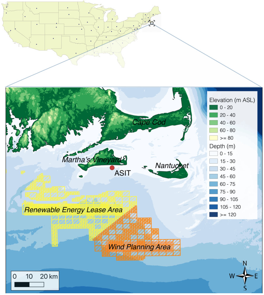 Figure 1
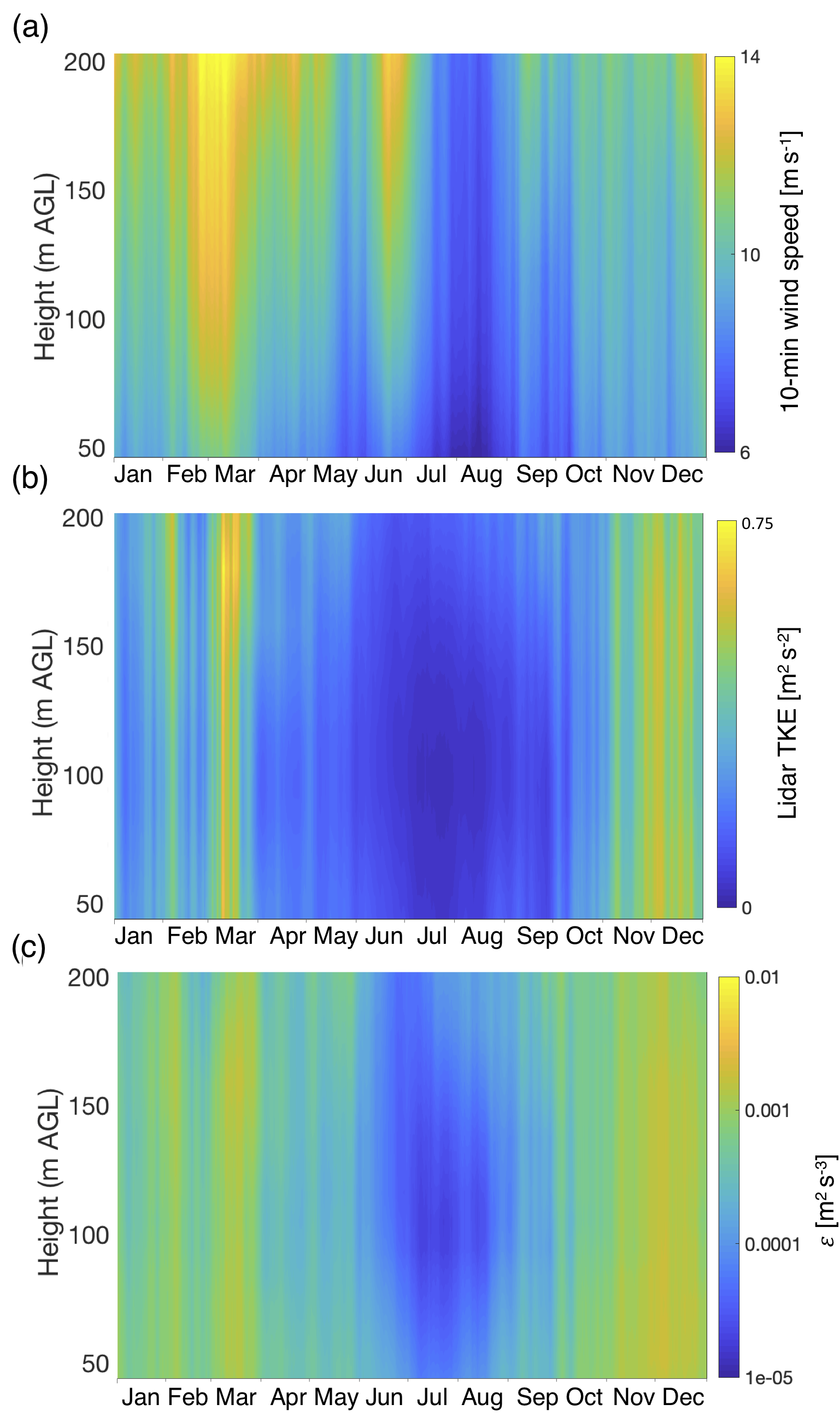 Figure 2
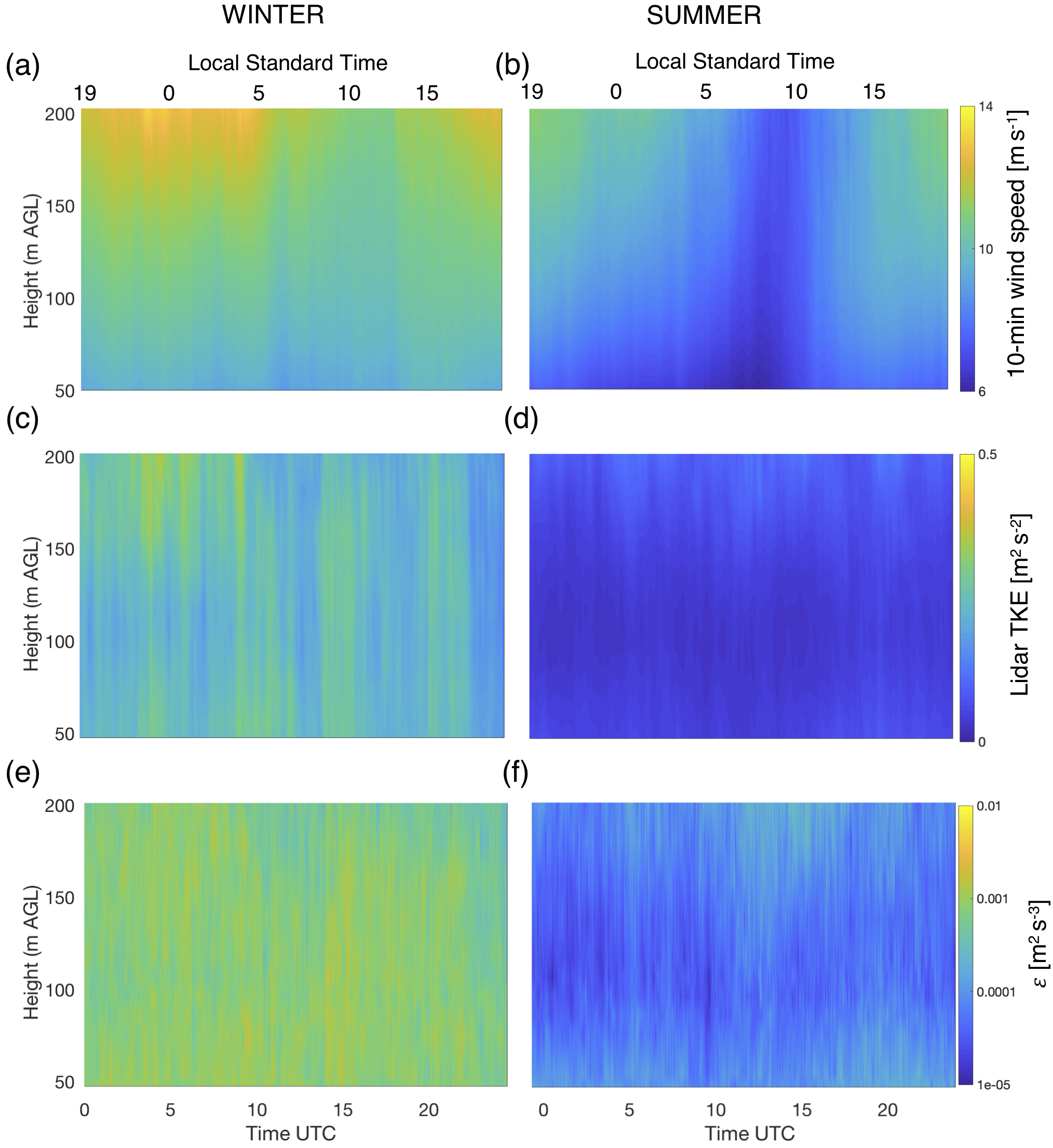 Figure 3
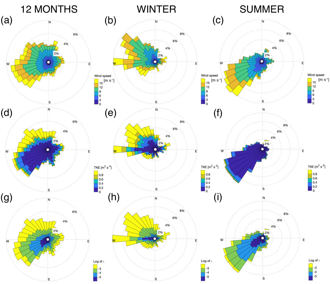 Figure 4
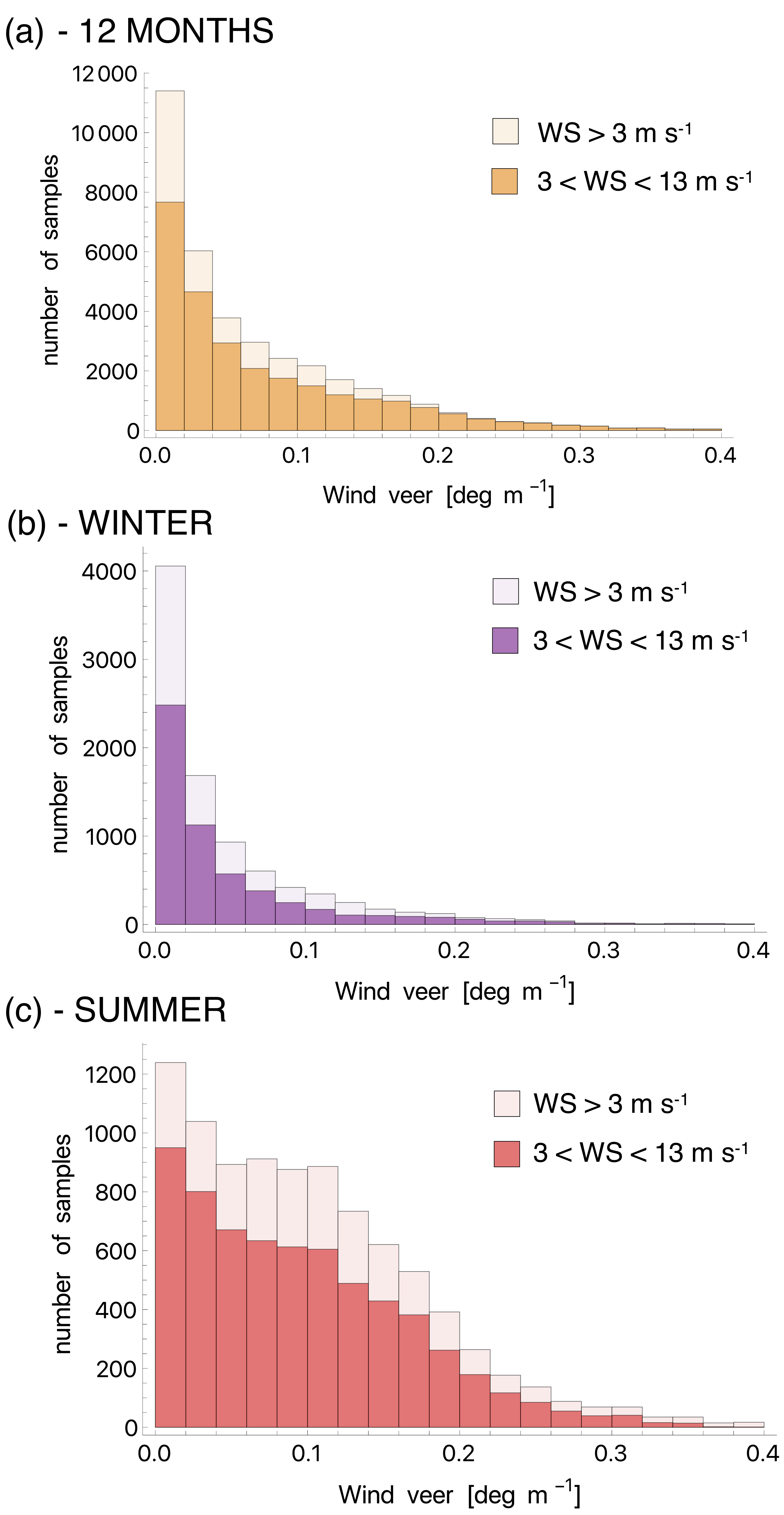 Figure 5
Peer Reviews
No public reviews on file for this paper yet. If you reviewed it on a platform where reviews are public (OpenReview, ICLR, NeurIPS, ICML), you can paste yours below so the community can read it here.
Videos
No videos yet. Explain this paper in a talk, walkthrough, or lecture? Add one.
Offshore Wind Turbines will encounter very low Atmospheric Turbulence
Abstract
The rapid growth of offshore wind energy requires accurate modeling of the wind resource, which can be depleted by wind farm wakes. Turbulence dissipation rate () governs the accuracy of model predictions of hub-height wind speed and the development and erosion of wakes. Here we assess the variability of turbulence kinetic energy and using 13 months of observations from a profiling lidar deployed on a platform off the Massachusetts coast. Offshore, is 2 orders of magnitude smaller than onshore, with a subtle diurnal cycle. Wind direction largely influences the annual cycle of turbulence, with larger values in winter when the wind flows from the land, and smaller values in summer, when the wind is mainly from open ocean. Because of the weak turbulence, wind plant wakes will be stronger and persist farther downwind in summer.
\draftfalse\journalname
Geophysical Research Letters
Department of Atmospheric and Oceanic Sciences, University of Colorado Boulder, Boulder, Colorado, USA National Renewable Energy Laboratory, Golden, Colorado, USA Woods Hole Oceanographic Institution, Woods Hole, Massachusetts, USA
\correspondingauthor
Nicola [email protected]
{keypoints}
strength and persistence of wind plant wakes depends on turbulence dissipation rate
turbulence dissipation rate offshore is small with a weak diurnal cycle
dissipation rate is larger when flow is from the land, which tends to be in wintertime at this site
1 Introduction
Wind energy continues to expand as one of the cleanest energy technologies, with its zero carbon emissions [Boyle (\APACyear2004)] and zero operational water consumption [Macknick \BOthers. (\APACyear2012)]. The faster and steadier winds which blow over the low-friction surface of the ocean [Landberg (\APACyear2015)] represent a valuable source of clean energy, especially given that the cost of offshore wind energy is decreasing faster than expected [Stiesdal (\APACyear2016)]. Many favorable locations for offshore wind farm development are close to coastal areas with large energy needs [Manwell \BOthers. (\APACyear2010)], minimizing the need for long-distance transmission [Wiser \BOthers. (\APACyear2015)].
Currently, most of the existing offshore wind farms are located in Northern Europe, where they account for a capacity of about 15 GW, with a planned increase to about 74 GW by 2030 [van Hoof (\APACyear2017)]. In the United States, only a single 30 MW commercial offshore wind farm [Deepwater Wind (\APACyear2016)] has been built. However, the U.S. offshore technical resource potential is estimated to be nearly double the nation’s current electricity use [Musial \BOthers. (\APACyear2016)]. Many offshore wind projects are currently being planned, mostly concentrated along the Eastern Seaboard. The State of Massachusetts plans to procure 1,600 MW of installed offshore wind, representing about 11% of its overall needs, by 2027 [Musial \BOthers. (\APACyear2017)], with beneficial impacts on the State’s economy and employment [Massachusetts Clean Energy Center \BOthers. (\APACyear2018)].
As offshore wind energy development grows, accurate forecasting of the available wind resource in the offshore environment is required. Recent studies [Yang \BOthers. (\APACyear2017), Berg \BOthers. (\APACyear2018)] have shown that the hub-height wind speed predicted by the Weather Research and Forecasting (WRF) model [Skamarock \BOthers. (\APACyear2005)] is highly sensitive to the parametrization of turbulence dissipation rate (), which is responsible for up to 50% of the variance in hub-height wind speed. Current parametrizations of assume a local balance between production and dissipation of turbulence within a grid cell. However, this assumption does not hold when using models at a fine horizontal resolution [Nakanishi \BBA Niino (\APACyear2006), Krishnamurthy \BOthers. (\APACyear2011), Hong \BBA Dudhia (\APACyear2012)]. Therefore, improved representations of in models are crucially needed to enhance the accuracy of wind energy forecasting.
Turbulence also plays a key role in the development and subsequent erosion of wind turbine and wind farm wakes, whose spatial extent has been observed to be particularly long offshore [Platis \BOthers. (\APACyear2018), Siedersleben, Platis\BCBL \BOthers. (\APACyear2018), Siedersleben, Lundquist\BCBL \BOthers. (\APACyear2018)], with observed wakes extending beyond 45 km in some cases. An accurate model representation of the turbulence dissipation rate would allow for a better layout optimization of offshore wind farms, which would in turn reduce the large costs related to wind farm wakes [Nygaard (\APACyear2014)] deriving from the uncoordinated development of wind projects [Lundquist \BOthers. (\APACyear2019)]. Therefore, an assessment of the variability of from observations in the offshore atmospheric boundary layer is an essential first step towards reducing uncertainty in offshore wind energy forecasting and optimizing energy production.
Various techniques to retrieve turbulence dissipation rates from sonic anemometers [Champagne \BOthers. (\APACyear1977), Oncley \BOthers. (\APACyear1996)], high-frequency hot-wire anemometers suspended on tethered lifting systems [Frehlich \BOthers. (\APACyear2006), Lundquist \BBA Bariteau (\APACyear2015)] or flown on aircrafts [Fairall \BOthers. (\APACyear1980)] or UAVs [Lawrence \BBA Balsley (\APACyear2013)] have been developed. The ease of deployment and extended measurement range of remote sensing instruments have also fueled research to derive methods to retrieve from lidars [Frehlich (\APACyear1994), Banakh \BOthers. (\APACyear1996), O’Connor \BOthers. (\APACyear2010), Wulfmeyer \BOthers. (\APACyear2016)] and radars [Shaw \BBA LeMone (\APACyear2003), McCaffrey \BOthers. (\APACyear2017)]. The extension and application of these techniques has led to a systematic assessment of the variability of in both flat [Bodini \BOthers. (\APACyear2018)] and complex terrain [Bodini \BOthers. (\APACyear2019)]. However, to the authors’ knowledge, no comprehensive analysis of the variability of turbulence dissipation rate in offshore environment has been completed.
Here, we assess the temporal variability of turbulence dissipation rate retrieved from 13 months of observations from a wind-profiling lidar deployed on an offshore platform. In Section 2 we describe the site off the Massachusetts coast, and the method used to retrieve . Section 3 presents the daily and seasonal variability of and its relation to wind direction and land influence. In Section 4 we summarize and conclude our analysis.
2 Data and Methods
2.1 The Massachusetts MetOcean Initiative
A ”MetOcean Initiative” [Filippelli \BOthers. (\APACyear2015)] funded by the Massachusetts Clean Energy Center has collected continuous observations of the atmospheric boundary layer at the Woods Hole Oceanographic Institution’s (WHOI) Air-Sea Interaction Tower (ASIT) since October 2016. The ASIT is a cabled, fixed platform located approximately 3 km south of Martha’s Vineyard in 17 m of water (Figure 1) and proximate to the Rhode Island and Massachusetts Wind Energy Areas, which represent the US’s largest region under development for offshore wind energy extraction. At the site, a suite of wind resource monitoring equipment was used to augment the existing sensors deployed by WHOI’s Martha’s Vineyard Coastal Observatory (MVCO), including a pair of cup anemometers above the top of the tower at 26 m above mean sea level (ASL), a wind vane at 23 m ASL, and a WINDUCUBE version (v2) profiling lidar on the main platform, at 13 m ASL. All metocean data collected by WHOI for the project was validated by AWS Truepower.
The v2 lidar measures line-of-sight velocity along the 4 cardinal directions with a nominal zenith angle of 28*∘*, with an additional line-of-sight velocity measurement along the vertical. The lidar was positioned on a platform extending away from the ASIT mast into the direction of prevailing winds (to the southwest) and rotated such that none of the measurement beams of the lidar were affected by the tower structure. Approximately 5 s are needed to complete the five-beam cycle. The lidar took measurements at 10 heights: 53, 60, 80, 90, 100, 120, 140, 160, 180, and 200 meters above sea level. Thus, the lidar-measured winds were above the level of, and not affected by the tower structure, nor were they expected to exhibit any signal of wave motion.
Here, the first 13 months of observations, from 7 October 2016 through 29 October 2017, have been analyzed. Periods during which precipitation was recorded at WHOI’s shore lab on the southern coast of Martha’s Vineyard have been excluded from the analysis.
2.2 Turbulence dissipation rate from profiling lidars
Turbulence dissipation rate can be estimated from the variance of the line-of-sight velocity measured by profiling lidars following the approach described in \citeAo2010method and refined in \citeAbodini2018estimation, with the assumption of locally homogeneous and isotropic turbulence. This approach derives by integrating the turbulence spectrum within the inertial subrange. To do so, the maximum length scale (and thus the sample size) to include in the calculation must be accurately chosen [Tonttila \BOthers. (\APACyear2015), Bodini \BOthers. (\APACyear2018)]. Here we use a local regression of the spectrum of the line-of-sight velocity to estimate the extension of the inertial subrange, as described and tested in \citeAbodini2019variability. The distribution of sample size values we obtain is between 20 s (5th percentile) and 300 s (95th percentile). is then calculated as
[TABLE]
where 0.52 is the one-dimensional Kolmogorov constant [Paquin \BBA Pond (\APACyear1971), Sreenivasan (\APACyear1995)], , with the horizontal wind speed and the dwell time, and , where is the size of the line-of-sight velocity sample determined from the local regression of the experimental spectra. The variance is calculated by subtracting a contribution due to the instrumental noise from the variance (averaged across the lidar beams) of line-of-sight velocity : , where is defined as in equation 2 in \citeApearson2009analysis. More details of this method are available in \citeAbodini2018estimation,bodini2019variability.
3 Results
Turbulence dissipation occurs in an environment determined by wind speed, whose annual cycle at the site is shown in Figure 2a (data have been smoothed with a 30-day running mean).
Wind speed is generally strong during winter, with average values above 10 m s*-1* at wind-turbine-hub-heights throughout the season, while summer shows smaller values, with minima in August, when the average wind speeds were less than 10 m s*-1* at every observed height. Turbulence quantities also exhibit an annual cycle. We calculate turbulence kinetic energy (TKE) as
[TABLE]
where the variances of the wind components are calculated over 2-min intervals. As noted by \citeAsathe2011can, lidars cannot fully resolve the wind variances, as a sonic anemometer would, given the lidars’ limited temporal frequency. However, since data from a sonic anemometer are not available in this case, we calculate TKE using data from the lidar, and will refer to it as lidar TKE [Rhodes \BBA Lundquist (\APACyear2013), Kumer \BOthers. (\APACyear2016)]. The annual cycle of lidar TKE (Figure 2b) reveals a clear pattern, with extremely small values during the summer, and larger values in winter, with little dependence on height. The annual variability of turbulence dissipation (Figure 2c) follows a similar pattern, and reaches maximum in fall and winter, with minima in the summer. Monthly average values of have a large correlation with monthly average lidar TKE (): when the kinetic energy of turbulence is on average large, large values of are usually needed to dissipate this energy. Monthly average wind speed has a slightly smaller correlation with (), with some considerable discrepancies (e.g. June). The annual cycle of at this offshore location differs from what was measured in similar campaigns onshore, where the annual cycle of is mainly driven by the seasonal cycle of convection, with larger turbulence in summer due to increased convection, and more quiescent conditions in winter due to higher stratification [Bodini \BOthers. (\APACyear2019)].
The annual variability of wind speed and turbulent properties at the site has a considerable impact on the average diurnal climatologies of these variables in different seasons (Figure 3).
Wind speed tends to increase during the late afternoon and at night, while in daytime conditions lower average wind speeds occur, with weaker shear, as also found by \citeAarcher2016predominance. On average, summer months (Figure 3b) show a larger diurnal cycle of wind speed compared to winter (Figure 3a). In contrast to this diurnal cycle in wind speed, the diurnal cycle of lidar TKE (Figure 3c and d) is subtle, with a small variability with height. The average diurnal cycles of offshore (Figure 3e and f) show similar patterns to lidar TKE, with differences greater than one order of magnitude between winter and summer. In summer, shows local minima at 100 m ASL, and increased values at 200 m ASL, especially in the local morning. In contrast, in winter shows a minimum in the morning at 200 m ASL. The average differences throughout the day in are smaller than one order of magnitude, whereas the diurnal cycle of onshore, in both flat [Bodini \BOthers. (\APACyear2018)] and complex [Bodini \BOthers. (\APACyear2019)] terrain, shows a larger amplitude, with differences of at least one order of magnitude between larger values during daytime and smaller values in nighttime quiescent conditions. Moreover, the average values of are smaller (in some cases of over an order of magnitude) than onshore [Bodini \BOthers. (\APACyear2018), Bodini \BOthers. (\APACyear2019)].
The summer minimum in lidar TKE and turbulence dissipation rate occurs because of wind regimes. North-westerly, westerly and south-westerly winds dominate at the ASIT site (Figure 4a). The wind direction dictates turbulence properties: north-westerly winds generally lead to large values of lidar TKE and . In contrast, south-westerly winds generally cause low turbulence regimes (panels d, g).
This relationship between wind direction and turbulence can be explained by considering the location of the ASIT platform (Figure 1). When the wind comes from the north-west, the flow interacts with the land before reaching the offshore platform. This land wake effect generates turbulence, both in terms of lidar TKE and . On the contrary, southwesterly winds come from the open ocean, where lower friction causes smaller values of lidar TKE and turbulence dissipation rates. In the summer (June, July, August), the winds consist of almost exclusively south-westerly winds (Figure 4c), associated with lidar TKE generally smaller than 0.2 m2 s*-2* (at 100 m ASL, Figure 4f) and turbulence dissipation rarely exceeding 10*-3* m2 s*-3* (Figure 4i). On the contrary, during the winter, northwesterly winds dominate (Figure 4b), with larger TKE (Figure 4c) and (Figure 4h). The annual cycle of turbulence dissipation rate offshore is more influenced by the wind-land interaction rather than the seasonal cycle itself.
An annual cycle also emerges in wind veer, another important atmospheric variable which affects the structure of wind turbine wakes [Bodini \BOthers. (\APACyear2017), Abkar \BOthers. (\APACyear2018), Churchfield \BBA Sirnivas (\APACyear2018)]. We calculate wind veer as the difference in 2-minute average wind direction, retrieved from the lidar, between 40 m and 200 m ASL, which represent typical vertical limits for the rotor of modern offshore wind turbine models. We present the observations as change in wind direction per meter of height (∘ m*-1*) to normalize the results in terms of the vertical separation between the measurements. Histograms of wind veer are shown in Figure 5, where we also highlight wind veer values which were measured with an average wind speed between 3 m s*-1* and 13 m s*-1*, which correspond to region 2, the area of the power curve where power is more sensitive to wind speed [Manwell \BOthers. (\APACyear2010)], of the Siemens Gamesa 7.0 MW turbine.
Wind veer often assumes large values between the considered vertical limits, with an average value of 0.07*∘* m*-1* (0.08*∘* m*-1* for region 2 wind speeds) when considering the whole period of observations (panel a). However, important differences between the seasons emerge. In winter months (panel b), the average wind veer wind observed (0.05*∘* m*-1*, 0.04*∘* m*-1* for regime 2 wind speeds) is only half of the summer average (0.10*∘* m*-1*, 0.09*∘* m*-1* for regime 2 wind speeds). The summertime offshore wind veer conditions are similar to the nighttime stable conditions found onshore in \citeAwalter2009speed. Veer is of particular interest with respect to wind turbine wake propagation [Bodini \BOthers. (\APACyear2017), Churchfield \BBA Sirnivas (\APACyear2018)], and wakes impact power production the most at wind speeds in region 2. The coupling of the strong veer in summertime conditions with low dissipation will result in long-propagating but skewed wakes, impacting power production and turbulent loads on downwind turbines.
4 Discussion and Conclusions
Offshore wind plant wakes can extend tens of km downwind [Platis \BOthers. (\APACyear2018), Siedersleben, Platis\BCBL \BOthers. (\APACyear2018), Siedersleben, Lundquist\BCBL \BOthers. (\APACyear2018)] in low-turbulence, stably-stratified conditions. These wakes undermine offshore power production [Nygaard (\APACyear2014)]. Because wind plant wake propagation is influenced by turbulence variability [Lundquist \BOthers. (\APACyear2019)], we assess the turbulence dissipation rate () from a year-long dataset of offshore wind lidar deployment.
We have retrieved from 13 months of observations from a profiling lidar located on an offshore platform 3 km south of Martha’s Vineyard, off the coast of Massachusetts. Offshore has, on average, smaller values compared to those found in comparable studies onshore, with a weak diurnal cycle. The small average values of are conducive to strong and long-lived wind plant wakes such as those wakes observed in stable stratification in the North Sea [Platis \BOthers. (\APACyear2018), Siedersleben, Platis\BCBL \BOthers. (\APACyear2018), Siedersleben, Lundquist\BCBL \BOthers. (\APACyear2018)]. Moreover, this extended persistence of wakes will be noticeable throughout the diurnal cycle, given the absence of strong turbulence dissipation even in convective daytime conditions. The seasonal cycle of is largely influenced by the dominant wind directions at the site. When the wind comes from the land, the interaction between the wind flow and the onshore topography increases the TKE (which has a large positive correlation with ) observed offshore and, consequently, turbulence dissipation. Therefore, the study of the optimal layout of offshore wind farms needs to consider the different turbulence regimes associated with the dominant wind patterns at each site, to possibly take advantage of the faster wake erosion connected to larger dissipation values caused by land wake effects.
While the offshore wind resource is considerable, and the daily timing of wind speed increases due to sea breeze effects in the summer are particularly valuable for integrating wind energy into power grids, these results suggest that flow from the south and southwest that would lead to increased wind speeds would also have reduced turbulence, leading to stronger and more persistent wind plant wakes. Moreover, wakes in the summer would be affected by wind veer greater than 14*∘* between the vertical limits of typical current commercial offshore wind turbines, and even larger values can be expected when considering wind gusts [Worsnop \BOthers. (\APACyear2017)]. This large wind veer can impact the effectiveness of wake steering solutions [Fleming \BOthers. (\APACyear2017), Fleming \BOthers. (\APACyear2019)] to minimize the wake energy loss.
Moreover, as the current wind farm lease areas are more than 25 km offshore of the platform where the profiling lidar was deployed, even the stronger turbulence conditions observed in the winter could represent an extreme upper bound on the boundary layer turbulence in the lease areas. The increased turbulence produced by the flow interaction with the land would likely dissipate as it flows offshore. As offshore wind plants in this region are developed, consideration of the likely persistence of wind plant wakes will be required to accurately predict the wind resource as well as the effect of skewed wakes on turbine operations and maintenance costs.
Given the complexity of the dependencies between and other atmospheric variables, as well as the importance of the interaction with the site-specific topography, the potential of sophisticated machine learning techniques could be tested to improve the model parametrizations of , as already successfully done with other atmospheric phenomena [Sharma \BOthers. (\APACyear2011), Xingjian \BOthers. (\APACyear2015), Alemany \BOthers. (\APACyear2018), Gentine \BOthers. (\APACyear2018)].
Acknowledgements.
Collection of the underlying wind data that provides the basis for this analysis was funded by the Massachusetts Clean Energy Center through agreements with the Woods Hole Oceanographic Institution and AWS Truepower. The authors appreciate the efforts of the MVCO/ASIT marine technicians at WHOI and AWS staff who helped collect the data. This analysis was supported by the National Science Foundation CAREER Award (AGS-1554055) to JKL and NB, and by internal funds from the Woods Hole Oceanographic Institution for AK. The lidar observations used here are available by contacting Dr. Kirincich directly ([email protected]).
The reference list from the paper itself. Each links out to its DOI / PubMed record.
- 1Abkar \B Others . ( \APA Cyear 2018) \APA Cinsertmetastar abkar 2018 analytical {APA Crefauthors} Abkar, M., Sørensen, J. \BCBL \BBA Porté-Agel, F. \APA Cref Year Month Day 2018. \BBOQ \APA Crefatitle An Analytical Model for the Effect of Vertical Wind Veer on Wind Turbine Wakes An analytical model for the effect of vertical wind veer on wind turbine wakes. \BBCQ \APA Cjournal Vol Num Pages Energies 1171838. \Print Back Refs \Current Bib
- 2Alemany \B Others . ( \APA Cyear 2018) \APA Cinsertmetastar alemany 2018 predicting {APA Crefauthors} Alemany, S., Beltran, J., Perez, A. \BCBL \BBA Ganzfried, S. \APA Cref Year Month Day 2018. \BBOQ \APA Crefatitle Predicting Hurricane Trajectories using a Recurrent Neural Network Predicting hurricane trajectories using a recurrent neural network. \BBCQ \APA Cjournal Vol Num Pages ar Xiv preprint ar Xiv:1802.02548. \Print Back Refs \Current Bib
- 3Archer \B Others . ( \APA Cyear 2016) \APA Cinsertmetastar archer 2016 predominance {APA Crefauthors} Archer, C \BPBI L., Colle, B \BPBI A., Veron, D \BPBI L., Veron, F. \BCBL \BBA Sienkiewicz, M \BPBI J. \APA Cref Year Month Day 2016. \BBOQ \APA Crefatitle On the predominance of unstable atmospheric conditions in the marine boundary layer offshore of the US northeastern coast On the predominance of unstable atmospheric conditions in the marine boundary layer offshore of the us northeastern
- 4Banakh \B Others . ( \APA Cyear 1996) \APA Cinsertmetastar banakh 1996 measurement {APA Crefauthors} Banakh, V., Werner, C., Köpp, F. \BCBL \BBA Smalikho, I. \APA Cref Year Month Day 1996. \BBOQ \APA Crefatitle Measurement of the turbulent energy dissipation rate with a scanning Doppler lidar Measurement of the turbulent energy dissipation rate with a scanning doppler lidar. \BBCQ \APA Cjournal Vol Num Pages ATMOSPHERIC AND OCEANIC OPTICS C/C OF OPTIKA ATMOSFERY I OKEANA 9849–853. \Print Ba
- 5Berg \B Others . ( \APA Cyear 2018) \APA Cinsertmetastar berg 2018 sensitivity {APA Crefauthors} Berg, L \BPBI K., Liu, Y., Yang, B., Qian, Y., Olson, J., Pekour, M. \BDBL Hou, Z. \APA Cref Year Month Day 2018. \BBOQ \APA Crefatitle Sensitivity of Turbine-Height Wind Speeds to Parameters in the Planetary Boundary-Layer Parametrization Used in the Weather Research and Forecasting Model: Extension to Wintertime Conditions Sensitivity of turbine-height wind speeds to parameters in the planetary b
- 6Bodini \B Others . ( \APA Cyear 2019) \APA Cinsertmetastar bodini 2019 variability {APA Crefauthors} Bodini, N., Lundquist, J \BPBI K., Krishnamurthy, R., Pekour, M. \BCBL \BBA Berg, L \BPBI K. \APA Cref Year Month Day 2019. \BBOQ \APA Crefatitle Spatial and temporal variability of turbulence dissipation rate in complex terrain Spatial and temporal variability of turbulence dissipation rate in complex terrain. \BBCQ \APA Cjournal Vol Num Pages Atmospheric Chemistry and Physics Discussionsi
- 7Bodini \B Others . ( \APA Cyear 2018) \APA Cinsertmetastar bodini 2018 estimation {APA Crefauthors} Bodini, N., Lundquist, J \BPBI K. \BCBL \BBA Newsom, R \BPBI K. \APA Cref Year Month Day 2018. \BBOQ \APA Crefatitle Estimation of turbulence dissipation rate and its variability from sonic anemometer and wind Doppler lidar during the XPIA field campaign Estimation of turbulence dissipation rate and its variability from sonic anemometer and wind doppler lidar during the XPIA field campaign. \
- 8Bodini \B Others . ( \APA Cyear 2017) \APA Cinsertmetastar bodini 2017 three {APA Crefauthors} Bodini, N., Zardi, D. \BCBL \BBA Lundquist, J \BPBI K. \APA Cref Year Month Day 2017. \BBOQ \APA Crefatitle Three-dimensional structure of wind turbine wakes as measured by scanning lidar Three-dimensional structure of wind turbine wakes as measured by scanning lidar. \BBCQ \APA Cjournal Vol Num Pages Atmospheric Measurement Techniques 108. \Print Back Refs \Current Bib