Matrix denoising for weighted loss functions and heterogeneous signals
William Leeb

TL;DR
This paper develops optimal spectral denoisers for low-rank matrix estimation under weighted loss functions, addressing challenges of heterogeneity, missing data, and heteroscedastic noise, to improve denoising performance.
Contribution
It introduces a framework for deriving optimal spectral denoisers for weighted loss functions and combines them to exploit heterogeneity in signals for enhanced estimation.
Findings
Derived optimal spectral denoisers for weighted loss functions.
Constructed a new denoiser leveraging heterogeneity to improve accuracy.
Addressed analysis challenges of non-orthogonally-invariant weighted losses.
Abstract
We consider the problem of estimating a low-rank matrix from a noisy observed matrix. Previous work has shown that the optimal method depends crucially on the choice of loss function. In this paper, we use a family of weighted loss functions, which arise naturally for problems such as submatrix denoising, denoising with heteroscedastic noise, and denoising with missing data. However, weighted loss functions are challenging to analyze because they are not orthogonally-invariant. We derive optimal spectral denoisers for these weighted loss functions. By combining different weights, we then use these optimal denoisers to construct a new denoiser that exploits heterogeneity in the signal matrix to boost estimation with unweighted loss.
Click any figure to enlarge with its caption.
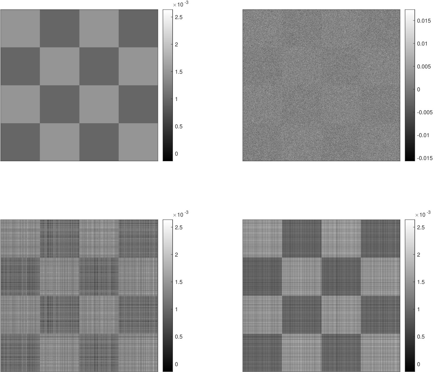 Figure 1
 Figure 2
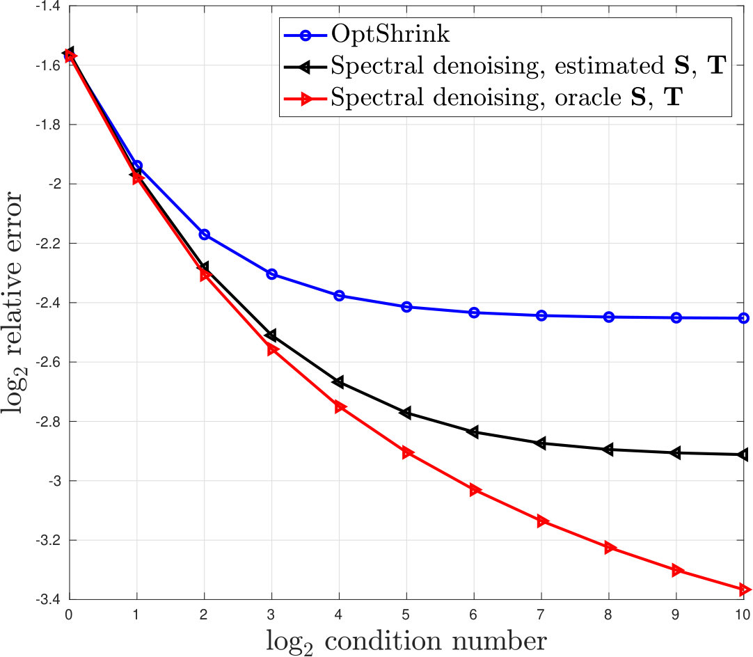 Figure 3
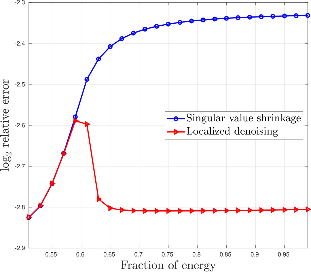 Figure 4
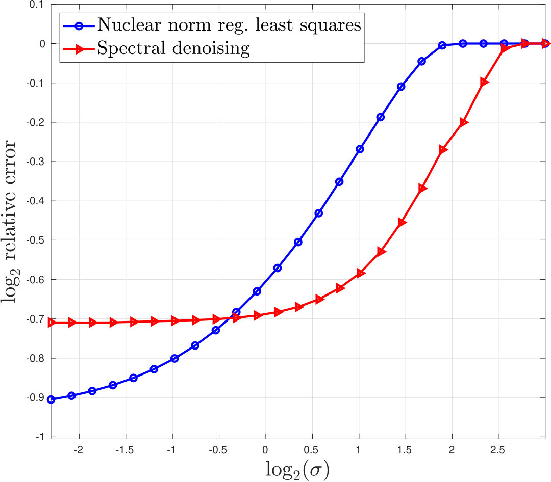 Figure 5
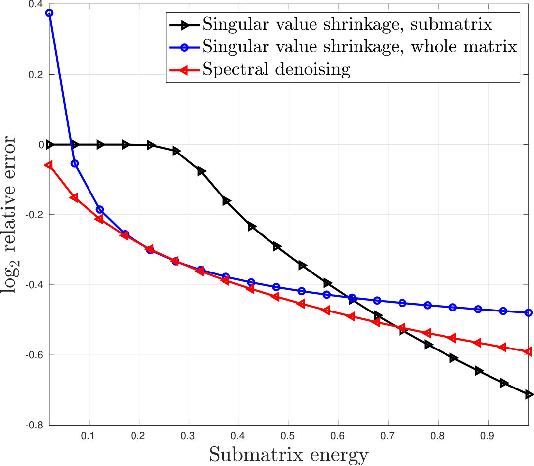 Figure 6
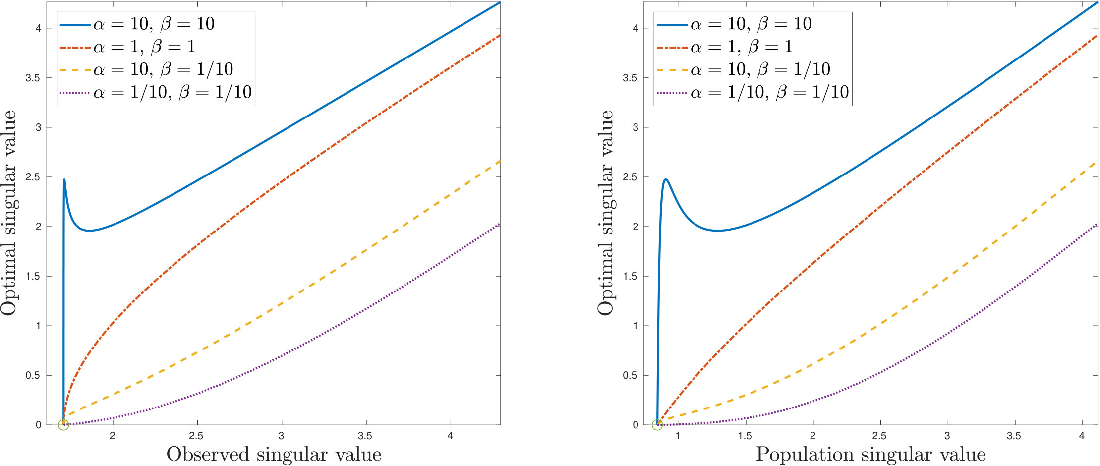 Figure 7
| Mean relative error, | ||||
|---|---|---|---|---|
| Gaussian | Rademacher | t, df=10 | t, df=3 | |
| 2.956e-02 | 3.057e-02 | 2.928e-02 | 3.284e-01 | |
| 2.050e-02 | 2.127e-02 | 2.042e-02 | 4.208e-01 | |
| 1.459e-02 | 1.514e-02 | 1.466e-02 | 5.280e-01 | |
| 1.033e-02 | 1.019e-02 | 1.030e-02 | 6.535e-01 | |
| 7.459e-03 | 7.693e-03 | 7.495e-03 | 7.640e-01 | |
| Mean relative error, | ||||
|---|---|---|---|---|
| Gaussian | Rademacher | t, df=10 | t, df=3 | |
| 1.991e-02 | 2.039e-02 | 1.975e-02 | 1.757e-01 | |
| 1.414e-02 | 1.437e-02 | 1.412e-02 | 2.219e-01 | |
| 9.917e-03 | 1.015e-02 | 1.001e-02 | 2.788e-01 | |
| 7.027e-03 | 6.875e-03 | 7.005e-03 | 3.455e-01 | |
| 5.040e-03 | 5.224e-03 | 5.087e-03 | 4.141e-01 | |
| Mean relative error | |||
|---|---|---|---|
| Noise type | Oracle | K-N | Naive |
| Gaussian | 4.010e-01 | 4.010e-01 | 4.012e-01 |
| Rademacher | 4.012e-01 | 4.012e-01 | 4.013e-01 |
| t, df=10 | 4.022e-01 | 4.022e-01 | 4.024e-01 |
| t, df=5 | 4.047e-01 | 4.086e-01 | 4.099e-01 |
| t, df=4 | 4.337e-01 | 4.484e-01 | 4.539e-01 |
| t, df=3 | 6.606e-01 | 7.459e-01 | 7.611e-01 |
| t, df=2.5 | 1.026e+00 | 1.287e+00 | 1.300e+00 |
| Mean rank | |||
|---|---|---|---|
| Noise type | Oracle | K-N | Naive |
| Gaussian | 2.000e+00 | 2.000e+00 | 2.084e+00 |
| Rademacher | 2.000e+00 | 2.000e+00 | 2.037e+00 |
| t, df=10 | 2.000e+00 | 2.000e+00 | 2.094e+00 |
| t, df=5 | 2.000e+00 | 2.128e+00 | 2.443e+00 |
| t, df=4 | 2.000e+00 | 2.858e+00 | 3.577e+00 |
| t, df=3 | 2.000e+00 | 7.875e+00 | 8.967e+00 |
| t, df=2.5 | 2.000e+00 | 1.643e+01 | 1.716e+01 |
Peer Reviews
No public reviews on file for this paper yet. If you reviewed it on a platform where reviews are public (OpenReview, ICLR, NeurIPS, ICML), you can paste yours below so the community can read it here.
Videos
No videos yet. Explain this paper in a talk, walkthrough, or lecture? Add one.
Matrix denoising for weighted loss functions and
heterogeneous signals
William Leeb School of Mathematics, University of Minnesota, Twin Cities. Minneapolis, MN.
Abstract
We consider the problem of estimating a low-rank matrix from a noisy observed matrix. Previous work has shown that the optimal method depends crucially on the choice of loss function. In this paper, we use a family of weighted loss functions, which arise naturally for problems such as submatrix denoising, denoising with heteroscedastic noise, and denoising with missing data. However, weighted loss functions are challenging to analyze because they are not orthogonally-invariant. We derive optimal spectral denoisers for these weighted loss functions. By combining different weights, we then use these optimal denoisers to construct a new denoiser that exploits heterogeneity in the signal matrix to boost estimation with unweighted loss.
1 Introduction
This paper is concerned with estimating a low-rank signal matrix from an observed matrix , where is a full-rank matrix of noise. We consider two distinct aspects of the matrix denoising problem. First, we study methods designed for a broader family of loss functions, known as weighted loss functions, than considered in earlier works. Second, we design a new denoiser for unweighted loss that improves upon previous work by exploiting heterogeneity in the target matrix’s singular vectors. Like many works on matrix denoising, our methods are designed for an asymptotic regime where the number of rows and columns of grow infinitely large, and where the energy in the noise swamps the energy in the signal. This setting is often referred to as the spiked model [4, 3, 5, 47, 29, 8].
The methods introduced in this paper extend singular value shrinkage [51, 20, 19, 43, 18, 38], which modifies ’s singular values to mitigate the effects of noise. Our method of spectral denoising agrees with singular value shrinkage with unweighted loss, but performs better with weighted loss. While weighted loss functions arise in a number of applications which we describe, they are challenging as they are not orthogonally-invariant. To derive optimal spectral denoisers for weighted loss, we extend the asymptotic theory of the spiked model, building on work from [40].
Our new method of localized denoising is designed for unweighted loss. Unlike singular value shrinkage, however, localized denoising exploits heterogeneity in ’s singular vectors; when certain blocks of coordinates of are known to contain more of the signal’s energy than others, localized denoising outperforms shrinkage. At the same time, localized denoising’s asymptotic performance is never worse than shrinkage’s, and so localized denoising inherits shrinkage’s well-known optimality properties.
1.1 Main ideas
In the high-noise, high-dimensional spiked model, the energy of the noise is unbounded as , while the energy of is fixed. Consistent estimation of from is therefore not possible, so the “best” denoiser depends on the choice of loss function. The weighted loss functions we use arise in a variety of applications, described in Section 6; the new method of spectral denoising is adapted to each of these. Table 1 lists these algorithms and their locations in the paper.
The optimal spectral denoiser for weighted loss solves a least-squares problem parameterized by weighted inner products between the singular vectors of and . Though formulas for unweighted inner products are well-known [47, 8], the results we need require a new analysis extending our earlier work in [40]. While we leave the details to Theorem 3.2, the key idea is that a singular vector of may be written as a combination of its projection onto the corresponding singular vector of and a residual unit vector , . Here, and are known from the classical theory of the spiked model [47]. Because the noise is orthogonally invariant, the are uniformly random in the subspace orthogonal to ’s singular vectors. Consequently, inner products of the form have predictable behavior when the dimension is large [21, 57, 49].
1.2 Illustrative example
The method of localized denoising, introduced in Section 5, uses the optimal spectral denoiser for weighted loss to construct a matrix denoiser for unweighted loss. The matrix is broken into submatrices, each of which is denoised by applying the optimal spectral denoiser with weights projecting onto that submatrix’s coordinates. In Figure 1, we illustrate the performance of localized denoising on the MIT logo, which is a -by- matrix with rank . The logo is corrupted by iid Gaussian noise with standard deviation , being the smallest singular value of the clean image. We apply optimal singular value shrinkage and localized denoising, the latter by breaking the rows into equispaced segments and the columns into equispaced segments. The relative error of localized denoising is approximately ; the relative error of singular value shrinkage is approximately , which is significantly larger. The improvement from localized denoising is due to the signal matrix’s heterogeneity along the rows and columns. However, the row and column subdivisions are not chosen to extract any specific structure in the image, and localized denoising does not appear to be very sensitive to the choice of subdivisions; similar results may be obtained with other subdivisions as well.
1.3 Outline of the paper
Section 2 contains the problem statement and key definitions. Section 3 presents the new asymptotic results. Section 4 derives the optimal spectral denoiser for weighted loss. Section 5 introduces localized denoising. Section 6 describes three applications of weighted loss functions. Section 7 reports on numerical experiments. Section 8 concludes by discussing potential applications.
2 Preliminaries
2.1 The observation model
We observe a -by- data matrix , consisting of a low-rank signal matrix and a full-rank isotropic Gaussian noise matrix . We write as where the and are orthonormal vectors in and , respectively, and . The entries of the noise matrix are iid . We write as where the and are orthonormal vectors in and , respectively, and .
We let be one of a sequence of matrices with columns, and be one of a sequence of matrices with columns. In Section 2.3, these matrices will be used to define the loss function for estimating . In order to have a well-defined asymptotic theory when , we assume that certain quantities defined in terms of , , and the singular vectors of have definite, finite limits. We define:
[TABLE]
For , we assume that the weighted inner products between the population singular vectors converge almost surely in the large , large limits:
[TABLE]
For , we will let and .
We assume that these limits exist and are finite and positive. We also assume that the operator norms of the matrices and remain bounded as ; that is, for all and , where does not depend on or . These conditions are the only assumptions we make on the matrices and .
We will parametrize the problem size by the number of columns , and let the number of rows grow with . Specifically, we will assume that the limit
[TABLE]
is well-defined and finite. In all statements where , it will be implicitly assumed as well that and . We assume that the number of population components and the singular values stay fixed with and .
Remark 1**.**
All quantities that depend on and , such as and , are actually elements of a sequence indexed by and/or . However, for notational simplicity, we drop the explicit dependence on and unless it is needed for clarity.
Remark 2**.**
There are counterexamples to the existence of the limits in (1) and (2). For example, one may take to be the first standard unit vector when is even, and the constant vector when is odd; and take . The limit defining will not exist in this case, as odd terms in the sequence converge to , and even terms converge to [math]. By contrast, the examples in Section 7 satisfy the asymptotic conditions.
Remark 3**.**
The values , , , and from equations (1) and (2) are used to characterize the weighted inner products between singular vectors of and ; see Theorem 3.2. These weighted inner products are needed to evaluate optimal spectral denoisers for weighted loss, as described in Section 4.
2.2 Heterogeneity, genericity, and weighted orthogonality
One of the aspects of the theory of matrix denoising we will explore is the role of the signal matrix ’s singular vectors, and . To that end, we introduce two definitions we will be using throughout the paper. We say that a unit vector is generic with respect to an -by- positive-semidefinite matrix if where “” indicates that the difference between the two sides vanishes almost surely as (to be precise, and are elements of a sequence of vectors and matrices, respectively, indexed by ; but following the convention described in Remark 1 we will drop the explicit dependence on ).
By contrast, we say that is heterogeneous if it is not generic. This means that the energy of the vector is not uniformly distributed across its coordinates in the eigenbasis of . Indeed, if is the eigendecomposition of , then
[TABLE]
If the energy of were equally spread out across the , then , and so .
Given a collection of vectors , we will say that they satisfy the weighted orthogonality condition (or are weighted orthogonal) with respect to a positive-semidefinite matrix if
[TABLE]
whenever . In other words, the are asymptotically orthogonal with respect to the weighted inner product defined by .
Remark 4**.**
From the Hanson-Wright inequality [21, 57, 49], random unit vectors from suitably regular distributions are generic, with respect to any with bounded operator norm. Furthermore, the weighted orthogonality condition will also hold for independent random unit vectors from a suitable distribution (see [7]).
2.3 Spectral denoisers and weighted loss functions
For the top empirical singular vectors and of , define the matrices and . Consider the class of estimators defined by
[TABLE]
Each matrix in has the same singular subspaces as the observed matrix , though not necessarily the same singular vectors. We call the family of spectral denoisers.
We consider estimating the low-rank signal matrix with respect to the weighted Frobenius loss defined by
[TABLE]
where denotes the matrix Frobenius norm, and and are matrices satisfying the conditions in Section 2.1. This type of loss function is used when the user pays different prices for errors in different rows and columns.
We now define the precise estimation problem we will consider. For any deterministic -by- matrix , we define the asymptotic error
[TABLE]
Our goal is then to find the matrix to minimize this loss, and show how may be consistently estimated from the observed matrix . That is, we define
[TABLE]
and define .
Remark 5**.**
For any deterministic , the asymptotic loss (8) exists and is finite almost surely, even though the matrices and are growing in size. It will be shown in Section 4 that since and each have rank at most , depends only on ; the entries of ; and the weighted inner products between the top singular vectors of and . It will follow from Theorem 3.2 that these inner products converge almost surely to finite limits, and consequently that the asymptotic loss (8) is well-defined almost surely.
3 Asymptotic theory for the spiked model
In this section, we derive the limits of inner products between the weighted population and empirical vectors. We define the cosines between the unweighted empirical and population vectors:
[TABLE]
Next we define weighted inner products between the population and empirical vectors:
[TABLE]
These are inner products with weight matrices and , respectively. We also define the weighted inner products between the empirical singular vectors:
[TABLE]
We let and , and similarly for the other terms.
Remark 6**.**
From Theorem 3.2 below, the limits (11) and (12) exist almost surely and are finite so long as the assumptions on and from Section 2.1 hold.
The first result provides formulas for and , and relates the singular values of to those of . It is well-known in the literature (see e.g. [47, 8]).
Proposition 3.1**.**
For , the singular value of converges almost surely as to , defined by:
[TABLE]
For , the limits (10) defining and almost surely exist and are given by the following expressions:
[TABLE]
and
[TABLE]
Remark 7**.**
While the signs of and are arbitrary, their product satisfies . We may therefore assume that and (see, e.g., [43]).
Theorem 3.2**.**
Suppose . Then the limits (11) and (12) almost surely exist and are equal to the following expressions:
[TABLE]
[TABLE]
[TABLE]
[TABLE]
The proof of Theorem 3.2 may be found in Section A.
Remark 8**.**
While the signs of inner products between singular vectors are arbitrary, Theorem 3.2 states that once the signs of and are fixed, the signs of , , and are determined.
4 Optimal spectral denoising
In this section, we derive the asymptotically optimal spectral denoiser with respect to the weighted loss (8), and show how to consistently estimate it from . We define the -by- weighted inner product matrices , , , , , and , and the vector of population singular values.
Theorem 4.1**.**
The optimal choice of is given by with weighted AMSE almost surely equal to
[TABLE]
The proof of Theorem 4.1 may be found in Section B.
The matrices , , , , , and and the singular values may be estimated using Proposition 3.1 and Theorem 3.2. First, from Proposition 3.1, we can estimate , and , so long as , i.e. if :
[TABLE]
Remark 9**.**
From Remark 7, we can take both and to be positive.
The values and are directly estimable, as they are the weighted inner products between the empirical singular vectors. We then estimate and , assuming :
[TABLE]
When , we take and (so long as and both exceed , i.e. and both exceed ). Finally, for all , we take and . The method is summarized in Algorithm 1.
4.1 Diagonal denoisers
In this section, we consider a subset of spectral denoisers, in which the matrix is required to be diagonal. More precisely, we search for a vector of real numbers, so that the estimator
[TABLE]
minimizes the AMSE .
Remark 10**.**
Optimal diagonal denoising cannot have better asymptotic performance than optimal spectral denoising, as the diagonal denoiser is a spectral denoiser. However, Theorem 4.2 below shows that under weighted orthogonality, the methods coincide; and the simplicity of makes it easier to analyze, which will be exploited in the proofs of Theorem 5.2 and Proposition 6.1 and the analysis of Section 4.2.
Theorem 4.2**.**
Suppose that either are weighted orthogonal with respect to , or are weighted orthogonal with respect to . Suppose too that , . Then the singular values , , of are:
[TABLE]
where , and are given by (21), and and are given by (22). The weighted AMSE is almost surely equal to
[TABLE]
If and are both weighted orthogonal with respect to and , respectively, then .
The proof of Theorem 4.2 is found in Section C.
4.2 Behavior of the optimal singular values
In this section, we assume either that ; or that are weighted orthogonal with respect to and are weighted orthogonal with respect to . In either case, the optimal spectral denoiser coincides with the optimal diagonal denoiser, and both are given by Theorem 4.2. Though this setting is quite restrictive, it permits us to exploit formula (24) for the optimal singular values to gain insight into the behavior of the optimal spectral denoiser. Propositions 4.3 and 4.4 describe the behavior of the optimal singular value in this setting. Because each depends only on the information specific to component , we will drop the subscript from the notation.
Proposition 4.3**.**
If either or , then . Conversely, for any fixed value of , there are sufficiently large values of and for which .
Proposition 4.4**.**
If or , then is an increasing function of .
The proofs of Propositions 4.3 and 4.4 may be found in Section D and Section E, respectively.
Remark 11**.**
From [51, 20, 43], the optimal singular value for unweighted Frobenius loss is , which is smaller than the observed singular value . Proposition 4.3 shows that with weighted loss, such shrinkage only occurs for small or .
The conclusion of Proposition 4.4 need not hold if and . In Figure 2 we plot the optimal , both as a function of the observed singular value and the population singular value , for various values of and (and ). The non-monotonicity is apparent when .
5 Localized denoising
In this section, we introduce a new procedure called localized denoising for estimating with unweighted Frobenius loss. As we will show, localized denoising is asymptotically never worse than optimal singular value shrinkage [20, 51], defined by where . Since singular value shrinkage is optimal for unweighted loss both in the minimax sense and when averaging over a uniform prior on and [18, 51], localized denoising inherits these same optimality properties. Furthermore, localized denoising can outperform singular value shrinkage when the singular vectors of are heterogeneous.
5.1 Definition of localized denoising
To define localized denoising, we expand the identity matrices and into sums of pairwise orthogonal projections and , where and are fixed. We require that and for ; and similarly for the .
We let denote the optimal spectral denoiser with respect to the weight matrices and . We then define the locally-denoised matrix:
[TABLE]
We summarize the localized denoising procedure in Algorithm 2.
5.2 Performance of localized denoising
The following results compare the behavior of the localized denoiser to the optimal singular value shrinker .
Theorem 5.1**.**
* almost surely as .*
Theorem 5.2**.**
Suppose that either are weighted orthogonal with respect to all , or are weighted orthogonal with respect to all . Then almost surely as , where , and if some is heterogeneous with respect to some or some is heterogeneous with respect to some .
In other words, unless all the are generic with respect to all of the and all the are generic with respect to all of the , localized denoising will outperform singular value shrinkage asymptotically. The proofs of Theorems 5.1 and 5.2 are found in Section F and Section G, respectively.
Remark 12**.**
The weighted orthogonality condition of Theorem 5.2 will hold if the columns of are drawn iid from a sufficiently well-behaved distribution in .
Remark 13**.**
To apply Theorem 5.2, the user must select projection matrices and with respect to which the singular vectors of are heterogeneous. Datasets are often drawn from different experimental regimes in genetic microarray experiments [27, 41, 50], single-cell RNA processing [52, 55], and medical imaging [35]. In these settings, it is known a priori that signal components will likely be heterogeneous across the different subpopulations, and localized shrinkage is a natural tool.
Remark 14**.**
Theorem 5.1 guarantees that even if the projection matrices and are not chosen judiciously (see Remark 13), the asymptotic performance of localized denoising is never worse than singular value shrinkage. In practice, localized denoising requires estimating more parameters than does shrinkage, and if and are sizeable relative to and its performance might be worse due to finite sample fluctations in these parameter estimates, especially when the singular vectors of do not exhibit strong heterogeneity with respect to the projections. For such an example, see Section 7.1, and specifically Remark 21. Though a detailed analysis of this topic is beyond the scope of the present work, in practice the user can compare these trade-offs via simulation to determine if localized denoising is appropriate for their problem size and the expected level of heterogeneity with respect to the projections.
6 Applications of weighted denoising
In this section, we describe three applications of weighted loss functions: submatrix denoising, denoising with heteroscedastic noise, and denoising with missing data. In these problems, we estimate a low-rank matrix with respect to unweighted Frobenius loss. However, an intermediate step of the estimation procedure requires the use of a weighted loss function.
6.1 Submatrix denoising
We suppose we observe a data matrix , but our goal is to estimate only a -by- submatrix of , where and . Denoting by the coordinate selection operator for the rows of the submatrix, and the coordinate selection operator for the columns of the submatrix, we may write the target submatrix as .
One approach is to estimate the entire matrix with respect to the weighted loss This loss only penalizes errors in the rows and columns of . If denotes the optimal spectral denoiser minimizing , we define our estimator . The method is summarized in Algorithm 3.
Another natural approach is to simply ignore the rows and columns outside of , and denoise directly by optimal singular value shrinkage to the matrix (defining ). We let denote this estimator.
In the following result, we make the same assumptions on and from Section 2.1. Note that , and .
Proposition 6.1**.**
Suppose are weighted orthogonal with respect to , and are weighted orthogonal with respect to . Suppose and for . Then where the strict inequality holds almost surely in the limit .
The proof of Proposition 6.1 is found in Section H.
Remark 15**.**
If and are generic with respect to and , respectively, then and . Proposition 6.1 requires the much weaker condition that and (note that and ). Informally, even if the fraction of the signal’s energy contained in is disproportionately large, it still pays to denoise using the entire observed matrix , rather than the submatrix alone.
It will follow from the proof of Proposition 6.1 that if and , then the singular vectors of are better approximated by computing the singular vectors of and projecting onto the images of and , respectively, rather than computing the singular vectors of the submatrix itself. More precisely, we will show that and are the singular vectors of , and that the vectors and are better correlated with and , respectively, then are the singular vectors of .
6.2 Doubly-heteroscedastic noise
We consider estimating a low-rank matrix from an observed matrix , where is a noise matrix of the form , has iid entries with distribution , and and are positive-definite matrices. We assume the eigenvalues of and remain in an interval for all and , where and are fixed independently of and . We refer to the matrix as doubly-heteroscedastic noise.
Remark 16**.**
This noise model generalizes two previous models of heteroscedastic noise in the context of principal component analysis [22, 23, 24, 58, 40]. In both, the matrix consists of random, iid signal vectors of the form where , are orthonormal vectors, and the are iid random variables with variance and mean [math]. The model from [58] and [40] takes , in which case the observations are of the form , where . By contrast, the papers [22, 23, 24] take , in which case the observations are of the form . The doubly-heteroscedastic noise model takes , which generalizes both these models.
We consider the following three-step procedure. First, we whiten the noise, replacing by defined by We may write , where and has iid entries. Next, we apply a denoiser to to estimate ; we denote this by , for tailored to removing white noise. Finally, we unwhiten to obtain our final estimate of .
The Frobenius loss between and may be written as follows:
[TABLE]
which is a weighted loss between and , with weights and . The denoiser should be chosen to minimize this weighted Frobenius loss. The procedure is summarized in Algorithm 4, where is taken to be optimal spectral denoising,
Remark 17**.**
The procedure of whitening, denoising, and unwhitening has been employed in recent papers on the spiked model; see, for instance, [42, 40, 16]. In particular, [40] shows several advantages of working with the whitened matrix when the noise is one-sided, such as improved estimation of the singular vectors of . By contrast, the paper [24] shows that whitening is suboptimal in certain settings.
6.2.1 Estimating and
The signal/noise decomposition is obviously not well-defined unless the user possesses some additional knowledge about the noise matrix . While a detailed treatment of this problem is outside the scope of this paper, we observe that in the large , large asymptotic limit, the matrices and may be replaced by estimators and consistent in operator norm; that is, almost surely
[TABLE]
Remark 18**.**
The matrices and may be replaced by, respectively, and for any . Without loss of generality, we may therefore assume that .
The next result describes a simple method for estimating and consistently in operator norm when both are diagonal and the singular vectors of are delocalized.
Proposition 6.2**.**
Suppose , and . For and , define the estimators
[TABLE]
and and let and . Then and are consistent estimators of and , respectively; that is, (28) holds almost surely.
The proof of Proposition 6.2 may be found in Section I.
Remark 19**.**
The values in (29) are the sample standard deviations of the rows of . Normalizing by is then an instance of standardization of the rows, a commonly used method in principal component analysis [30].
Remark 20**.**
The estimates and capture the variation of both the noise and the signal. Proposition 6.2 states that if the signal is delocalized, then in the large , large limit its contribution becomes negligible. However, for finite and , and will still see the effects of the signal, and may not be good estimates of and . The experiment in Section 7.3 compares the use of the true and to their estimates.
6.2.2 Whitening increases the SNR for generic signal matrices
We show that the whitening transformation increases a natural signal-to-noise ratio of the observed matrix. We will assume throughout this section that the (respectively, ) are generic with respect to (respectively, ), and that they satisfy the pairwise orthogonality condition with respect to (respectively ). Writing the SVD of as we define the signal-to-noise ratio (SNR) for component of :
[TABLE]
which is the ratio of the squared operator norm of the component of and the squared operator norm of the noise.
Whitening turns into , with where , , and . The SNR after whitening is then:
[TABLE]
Define
[TABLE]
Note that from Jensen’s inequality, , and if either or is not a multiple of the identity. The following result extends an analogous finding from [40]:
Proposition 6.3**.**
Suppose are generic and weighted orthogonal with respect to , and are generic and weighted orthogonal with respect to . Then , almost surely as . In particular, is larger than if either or is not a multiple of the identity.
In other words, the SNR increases after whitening the noise by at least a factor of ; energy is transferred from the noise component to the signal component. The proof of Proposition 6.3, which extends an analogous result in [40], is in Section J.
6.3 Matrices with missing/unobserved values
We consider the setting where is a low-rank target matrix we wish to recover and is a matrix of iid Gaussian entries, but rather than observe , we observe only some subset of the entries. The problem of estimating a matrix from a subset of its entries is known as matrix completion [48, 32, 25, 13, 14, 12, 13, 33, 31, 11, 16, 34, 44, 53].
In this section, we will adopt a heterogeneous, rank 1 sampling model, as in [14]. We suppose that the rows and columns are sampled independently, with row sampled with probability , and column sampled with probability ; that is, entry of is sampled with probability . We observe the vector of sampled entries, where is the subsampling operator.
Following the approach from [16], we consider the backprojected matrix , in which the unobserved entries are replaced by [math]’s. We write . We show that asymptotically, behaves like the matrix . More precisely, we have the following result:
Proposition 6.4**.**
Suppose . Then in the limit , almost surely.
The proof of Proposition 6.4 may be found in Section K. It is a straightforward generalization of the analogous one-sided result in [16].
Let . Writing , we have , where is if entry is sampled, and [math] otherwise. Then has variance . Consequently, we can whiten the noise by applying and ; Proposition 6.3 suggests this will improve estimation of the matrix. To that end, we define where , and . Then is a random matrix where each entry has mean zero and variance .
From Proposition 6.4, asymptotically the matrix behaves like , and so denoising estimates of . To estimate we should perform denoising to with respect to the weighted loss function with weight matrices and . We then apply and to the resulting matrix, to obtain an estimator of itself. The method is summarized in Algorithm 5, where is the optimal spectral denoiser.
7 Numerical results
In this section, we report on numerical simulations demonstrating the performance of the algorithms from this paper.
7.1 Localized denoising
We evaluate the performance of localized denoising (Algorithm 2). We generate a “checkerboard” signal matrix of size -by-, , shown in the top left panel of Figure 4. Each light square has the same value, as does each dark square. For a specified number , the total energy of the light squares is of the total energy of . The Frobenius norm of is normalized to be . Whenever , is rank ; when , has constant value and is rank . We add a matrix of Gaussian noise, whose entries have standard deviation .
We estimate from using two methods: singular value shrinkage [20, 51] and localized denoising. Localized denoising is applied with row projection matrices , , that project onto equispaced blocks of rows, and column projection matrices , , that project onto equispaced blocks of columns. For each , the experiment is repeated times; the mean errors are plotted in Figure 3.
As increases, localized denoising outperforms singular value shrinkage more dramatically. This is because localized denoising uses a priori knowledge of ’s block structure, which becomes more pronounced as grows. Figure 4 shows an example of images of the true matrix , the noisy matrix , and the two denoised matrices, when . In this example, the relative error of localized denoising is approximately , whereas the shrinkage error is .
Remark 21**.**
The error curves in Figure 3 both appear nearly identical when , after which localized denoising begins to outperform singular value shrinkage. This is because for small values of the smallest singular value of is not detectable, and so both methods treat the matrix as a constant, rank matrix. Though not apparent from the plot, when the performance of singular value shrinkage is slightly better than localized denoising, due to finite sample fluctuations (see Remark 14). For example, when , the mean relative error of localized denoising is approximately , while that of shrinkage is approximately .
7.2 Submatrix denoising
We evaluate the performance of spectral denoising for estimating a submatrix contained within a larger matrix (Algorithm 3). We generate a rank 1 signal matrix of size -by-, , , with singular values , where . For a specified , the left singular vector of is piecewise constant on the two sets of coordinates and ; the values are such that the energy of on coordinates is equal to . Similarly, the right singular vector of is piecewise constant on the two sets of coordinates and , with values such that the energy of on is also equal to . Denoting by the -by- upper-left submatrix of , .
The noise matrix has Gaussian entries with variance . We denoise the submatrix using Algorithm 3; optimal singular value shrinkage [20, 51] on alone (“submatrix shrinkage”); and optimal singular value shrinkage on followed by projection onto the rows and columns of (“global shrinkage”). For each , the experiment is repeated for draws. Figure 5 plots the mean relative errors.
Optimal spectral denoising outperforms global shrinkage for all , since singular value shrinkage is an instance of spectral denoising and hence will not do better than the optimal spectral denoiser. Optimal spectral denoising and global shrinkage perform nearly identically when , since in this regime the singular vectors of are constant, and hence generic with respect to the weight matrices.
For small , the relative error of global shrinkage exceeds , since the submatrix’s energy is very small compared to the rest of the matrix. By contrast, optimal spectral denoising with weights and highlights the rows and columns in .
Optimal spectral denoising outperforms submatrix shrinkage except when is close to . This is consistent with Proposition 6.1, which states that unless the energy of ’s singular vectors are highly concentrated in the rows and columns of , optimal spectral denoising will outperform singular value shrinkage on the submatrix.
Finally, optimal singular value shrinkage on the submatrix has relative error when is small. This is because singular value shrinkage on the submatrix only computes the SVD of , not ; when the energy in the submatrix is too weak (i.e. is too small), no signal will be detected in the submatrix alone. By contrast, the singular values of the full matrix always reveal the presence of signal.
7.3 Doubly-heteroscedastic noise
We examine the performance of Algorithm 4. We generate a -by- signal matrix , , , of rank , with singular values , , where is the smallest singular detectable value of , evaluated using the method in [39]. Both the left and right singular vectors of are random orthonormal vectors in and , respectively.
For specified , we generate row and column diagonal covariance matrices and , each with eigenvalues linearly spaced between and . The noise matrix is , where has iid Gaussian entries with variance . We apply three denoising schemes: Algorithm 4 with the true and ; Algorithm 4 with and estimated using the method described in Proposition 6.2; and OptShrink [43]. The experiment is repeated times for each value of .
Figure 6 shows the mean relative errors of each method as a function of . For this model of and , the condition number is an increasing function of the parameter from Section 6.2.2. Consequently, Proposition 6.3 suggests that whitening will improve the matrix SNR, and that the improvement should increase as grows. This is precisely what Figure 6 demonstrates; optimal spectral denoising with whitening by and does indeed outperform OptShrink, and the performance gap grows with . Using the estimated covariances, the performance is degraded but still outperforms OptShrink when is large.
7.4 Missing data
We test spectral denoising for missing data (Algorithm 5) by comparing it to nuclear-norm regularized least-squares [11], which estimates by:
[TABLE]
Here, denotes the nuclear norm; is the projection operator onto the observed samples; and and are the diagonal matrices of sampling probabilities for rows and columns, respectively. We weight the nuclear norm by the square root of the sampling probabilities, as suggested in [14]. Following [11], we choose the parameter so that when is pure noise, is set to zero. It follows from the KKT conditions [10] that this is equivalent to which is approximated by . We solve (33) using the algorithm in [26].
We generate a rank signal matrix of size -by-, , , with singular values , , . Both the left and right singular vectors of are uniformly random. We add to a Gaussian noise matrix , where each entry has variance for a specified value of . is then subsampled with row and column sampling probabilities each equispaced between and . For each value of , the experiment is repeated 50 times. Figure 7 displays the mean relative errors. When is large, spectral denoising is superior, whereas in the small regime nuclear-norm regularized least-squares is better.
7.5 Non-Gaussian noise
The optimal spectral denoiser requires estimation of the weighted inner product matrices , , and . The formulas for the entries of these matrices provided by Theorem 3.2 assumes that the noise matrix is Gaussian. However, it is of interest whether the same formulas may be applied to non-Gaussian noise. To partially address this question, we compare the finite sample accuracy of the formulas in Theorem 3.2 for different noise distributions.
For each , we generate of size -by-, where . The signal has rank , with singular values and ; is uniformly equal to , and is on entries , and on entries . and are generated similarly, with in place of . The noise matrix has iid entries of variance , drawn from a specified distribution: Gaussian, Rademacher, t10 or t3, where the t distributions are normalized to have variance .
The -by- weight matrix is diagonal with diagonal entries equal to , and the remaining entries [math]. We evaluate the true matrix and use formulas (16) and (18) to predict and . For each draw, we compute the actual inner product matrices and using the left singular vectors and of . Due to the ambiguity in signs, we make all entries of the matrices positive. We then compute the relative errors and .
For each noise type and each value of , , the experiment is repeated 1000 times. The average and maximum relative errors are recorded in Table 2 for , and in Table 3 for . Both the average and maximum errors for Gaussian noise very nearly match those for the Rademacher and t10 distributions. However, the errors for the heavier tailed t3 distribution are much larger, indicating that the theory breaks down for this noise model. The errors for the Gaussian, Rademacher, and t10 distributions appear to decay approximately like ; this is the rate we expect from [6] and Theorem 2.19 in [8]. The errors for the t3 distribution do not exhibit such decay with increasing , indicating that the model does not match.
7.6 Rank estimation
In this section, we explore estimation of the rank of from the observed matrix , a topic that has received considerable attention [36, 37, 17, 15, 46, 45]. The naive estimator is defined by
[TABLE]
this simply counts the number of ’s singular values exceeding , the asymptotically largest singular value of the noise matrix . It is known that may overestimate the rank; see, e.g., [28]. The rank estimator of Kritchman and Nadler from [36], denoted by , is designed to prevent attributing noisy singular values to signal. We compare the performance of and for different noise distributions in terms of the accuracy of estimating and the effect on the denoising error.
For and , we generate a -by- signal matrix with rank and singular values and . The left singular vector is uniformly equal to , and is on entries , and on entries . The right singular vectors and are generated the same way, with in place of . The noise matrix had iid entries of variance , drawn from one a specified distribution, namely: Gaussian, Rademacher, or the t distributions with , , , and degrees of freedom, where the t distributions are normalized to have variance . The -by- weight matrix is diagonal with diagonal entries linearly spaced between and . The -by- weight matrix is also diagonal, with diagonal entries linearly spaced between and . In each run, we apply Algorithm 1 with the oracle , the naive from (34), and from [36], with confidence level111The code for computing was taken from Boaz Nadler’s website: www.wisdom.weizmann.ac.il/~nadler/Rank_Estimation/rank_estimation.html. For each noise distribution, the experiment is repeated times. In Tables 4 and 5 we record the relative errors and the estimated ranks.
For the Gaussian, Rademacher, and t10 distributions, the Kritchman-Nadler estimate is typically closer to the true rank, , than is the naive estimate . However, the average and maximum errors are close regardless of the rank estimator used, since even when , the third singular value of is so close to the detection edge that the estimates of the cosines and are nearly [math]. With the t5 distribution, both and are more likely to overestimate the true rank. While the average errors are close to those for the Gaussian, Rademacher, and t10 distributions, the maximum errors are much larger, indicating that while this noise distribution’s “typical” behavior may be close to the thinner tailed ones, a small number of extreme draws of can result in very poor performance. For the t distributions with , , and degrees of freedom, both and drastically overestimate the rank, and the resulting relative errors are enormous.
8 Conclusion
This paper has introduced a family of spectral denoisers for low-rank matrix estimation, which generalizes singular value shrinkage. We have derived optimal spectral denoisers for weighted loss functions, and discussed applications. By judiciously combining these denoisers for different weights we contructed the method of localized denoising, which outperforms singular value shrinkage under heterogeneity. While this paper has focused on theoretical and algorithmic development, in future work we plan to apply the methods to problems where related but suboptimal methods have previously been employed. This includes the problems of denoising and deconvolution of images from cryoelectron microscopy [9]; 3-D reconstruction of heterogeneous molecules from noisy images [1]; and denoising XFEL images [42, 59].
Acknowledgements
I thank Elad Romanov and Amit Singer for stimulating discussions related to this work, Edgar Dobriban for valuable feedback on an earlier version of this manuscript, and the reviewers for their helpful comments. I acknowledge support from the NSF BIGDATA award IIS 1837992 and BSF award 2018230.
Appendix A Proof of Theorem 3.2
The proof of Theorem 3.2 is similar to the analysis found in [40], in that it rests on the same decomposition of the empirical singular vectors and into the signal and residual components. If and are vectors of the same dimension, we will write as a short-hand for almost surely as . The statements are symmetric in the left and right singular vectors, so for compactness we will only prove them for the left ones. The proofs for the other side are identical.
Because the noise matrix has an isotropic distribution, we can write:
[TABLE]
where is a unit vector that is uniformly random over the sphere in the subspace orthogonal to (see [47]). Because is uniformly random, it is asymptotically orthogonal to any independent unit vector ; that is,
[TABLE]
Furthermore, satisfies the normalized trace formula, namely if is any matrix with bounded operator norm, then
[TABLE]
We refer the reader to [7, 21, 57, 49] for details. We will use (36) and (37) repeatedly. Furthermore, when it follows from Lemma A.2 in [40] that
[TABLE]
Applying to each side of (35), we have:
[TABLE]
The proofs of the identities in Theorem 3.2 now follow by manipulating the asymptotic equation (39) appropriately, in conjunction with (36), (37) and (38).
We first show the formulas for . We take inner products of each side of (39) with :
[TABLE]
where we have used (36).
To derive the formula for , we take the squared norm of each side of (39):
[TABLE]
The first asymptotic equivalence follows from (36), and the second from (37).
Finally, we derive the formula for , . From (39), we have
[TABLE]
From (36) and (38), the terms involving and vanish, and we are left with
[TABLE]
This completes the proof of Theorem 3.2.
Appendix B Proof of Theorem 4.1
The target matrix may be written
[TABLE]
and our estimate is of the form
[TABLE]
where , , , , and .
Define , , , and . We may then write the weighted loss as follows:
[TABLE]
which is the unweighted Frobenius loss between and . Continuing, we have:
[TABLE]
Defining the operator by , the pseudoinverse of is given by . Consequently, the choice of that minimizes is given by:
[TABLE]
The error may then be evaluated by substituting this expression for into (B), completing the proof.
Appendix C Proof of Theorem 4.2
Under weighted orthogonality, whenever , and so when as well. Consequently, the matrices , , , , , and are diagonal. The optimal is given by:
[TABLE]
which is also diagonal, with diagonal entries
[TABLE]
which is the desired expression.
Appendix D Proof of Proposition 4.3
Suppose a coordinate has signal strength (we drop the subscript as we are only considering one component). We may assume without loss of generality (and by rescaling and ) that . Consequently, the optimal singular value is equal to:
[TABLE]
By taking and sufficiently large, this value can be made arbitrarily close to
[TABLE]
That is, the optimal singular value will be greater than the observed singular value in this parameter regime.
On the other hand, if , we have:
[TABLE]
which shows that . A nearly identical proof works if . This completes the proof.
Appendix E Proof of Proposition 4.4
Without loss of generality, we will assume . We consider the functions and . Define the functions and by
[TABLE]
and
[TABLE]
Then we may write the optimal singular value as a function as follows:
[TABLE]
Let us assume that ; the proof for will be nearly identical. We wish to show that , for . We have
[TABLE]
and since , we must show that the right side is positive. It is straightforward to verify that
[TABLE]
from which it follows that
[TABLE]
Similarly, we can show
[TABLE]
Consequently, it is enough to show
[TABLE]
Direction computation shows
[TABLE]
and
[TABLE]
Substituting (62) and (63) into the left side of (61) and multiplying by , we get:
[TABLE]
which is the desired result.
Appendix F Proof of Theorem 5.1
We denote by the singular values of , and . We may then write
[TABLE]
This is a spectral denoiser (in the set ), and hence its weighted loss with weights and cannot be less than that of the optimal spectral denoiser . That is,
[TABLE]
Because the and are pairwise orthogonal projections which sum to the identity, the total Frobenius loss can be decomposed:
[TABLE]
which is the desired inequality.
Appendix G Proof of Theorem 5.2
For , , and , let , , , and . Then
[TABLE]
Let be the optimal diagonal denoiser with weights and . Because of the weighted orthogonality condition, Theorem 4.2 states that the AMSE for is
[TABLE]
Since minimizes the weighted error with weights and , we have:
[TABLE]
On the other hand, the error obtained by is equal to
[TABLE]
Comparing (G) and (71), the result will follow if we can show that for each ,
[TABLE]
where the inequality is strict so long as one of or is not generic with respect to some or ; or equivalently, either for some , or for some . Because
[TABLE]
it is enough to show that
[TABLE]
with the inequality being strict so long as for some .
For each , let . Then
[TABLE]
The function is convex. Since , Jensen’s inequality implies
[TABLE]
which is the desired inequality. The inequality will be strict so long as is not constantly equal to over , or equivalently if for some . This is the desired result.
Appendix H Proof of Proposition 6.1
Since has only columns, to ensure that the scaling of the noise matches that of the standard spiked model, we must multiply it by . We define and . Then follows a standard spiked model with signal matrix .
For , we let and denote the singular vectors of ; and denote the singular vectors of ; and denote the singular vectors of (and ); and and denote the singular vectors of (and ). We let denote the singular values of . We also let be the aspect ratio of the submatrix.
If are the singular values of the full -by- signal matrix , then we may write the rescaled submatrix as
[TABLE]
Because the and are assumed to by pairwise orthogonal, (77) is the SVD of . Consequently:
[TABLE]
We define the cosines
[TABLE]
Following Remark 7, we may assume that the singular vectors have been chosen so that both and are non-negative. Then the AMSE obtained by first applying optimal singular value shrinkage to , and then rescaling by , is
[TABLE]
We now turn to the weighted estimator . From the weighted orthogonality condition, , the optimal diagonal denoiser. From Theorem 4.2, the AMSE of may be written
[TABLE]
Comparing (80) and (81), the result will be proven if we can show
[TABLE]
and
[TABLE]
By the symmetry in the problem, it is enough to prove (82). Because we are working with each singular component separately, we will drop the subscript . From Proposition 3.1, the formula for is given by
[TABLE]
If , then (82) is trivial. Consequently, we assume . Because and , this is equivalent to the condition
[TABLE]
Defining , we may consequently assume that
[TABLE]
We may rewrite in terms of as follows:
[TABLE]
From the formula
[TABLE]
we may rewrite the right side of (82) as
[TABLE]
Comparing (87) to (89), the inequality (82) is equivalent to showing
[TABLE]
Because each side is affine linear in , and , it is enough to verify (90) at and . When , the left side of (90) is [math], whereas the right side is non-negative because and , verifying the inequality in this case. When , the difference between the right side and left side of (90), divided by , is equal to
[TABLE]
Since and , this expression is positive, verifying (90) and completing the proof.
Appendix I Proof of Proposition 6.2
From a standard Bernstein-type inequality for subexponential random variables (e.g. Proposition 5.16 from [56]), for every we have:
[TABLE]
for constants . Since , the right hand side is summable in ; it follows from the Borel-Cantelli Lemma that almost surely as . From the delocalization of ’s singular vectors, . Since , we then have
[TABLE]
Consequently, almost surely, as desired. Similar reasoning also shows that almost surely as . A nearly identical argument applied to the numerator of then shows almost surely, completing the proof.
Appendix J Proof of Proposition 6.3
To prove Proposition 6.3,we begin by deriving a lower bound on the operator norm of the noise matrix . We let and be unit vectors so that . Then
[TABLE]
Next, we take unit vectors and so that . Then we have
[TABLE]
Since the distribution of is orthogonally-invariant, the distributions of and are uniform over the unit spheres in and , respectively. Consequently, and . Therefore,
[TABLE]
where the inequality holds almost surely in the large , large limit. Note that (see, e.g., [2]), though we do not need to use this fact.
Furthermore, we also have
[TABLE]
Consequently,
[TABLE]
completing the proof.
Appendix K Proof of Proposition 6.4
Let be if entry is sampled, and [math] otherwise. Then . Let ; then , where denotes the Hadamard product. Let and . The matrix is a random matrix with mean zero, whose entries are uniformly bounded. It follows from Corollary 2.3.5 of [54] that a.s. as , for some constant .
We may write , and consequently . Since , it is enough to show that
[TABLE]
almost surely, for each .
Suppose and are two unit vectors. Then
[TABLE]
almost surely as .
Now, since is a unit vector,
[TABLE]
and similarly,
[TABLE]
Since , the result follows.
The reference list from the paper itself. Each links out to its DOI / PubMed record.
- 1[1] Joakim Andén and Amit Singer. Structural variability from noisy tomographic projections. SIAM Journal on Imaging Sciences , 11(2):1441–1492, 2018.
- 2[2] Zhidong Bai and Jack W. Silverstein. Spectral analysis of large dimensional random matrices . Springer Series in Statistics. Springer, 2009.
- 3[3] Zhidong Bai and Jian-feng Yao. Central limit theorems for eigenvalues in a spiked population model. Annales de l’Institut Henri Poincaré, Probabilités et Statistiques , 44(3):447–474, 2008.
- 4[4] Zhidong Bai and Jian-feng Yao. On sample eigenvalues in a generalized spiked population model. Journal of Multivariate Analysis , 106:167–177, 2012.
- 5[5] Jinho Baik and Jack W. Silverstein. Eigenvalues of large sample covariance matrices of spiked population models. Journal of Multivariate Analysis , 97(6):1382–1408, 2006.
- 6[6] Zhigang Bao, Xiucai Ding, and Ke Wang. Singular vector and singular subspace distribution for the matrix denoising model. ar Xiv preprint ar Xiv:1809.10476 , 2018.
- 7[7] Florent Benaych-Georges, Alice Guionnet, and Myléne Maida. Fluctuations of the extreme eigenvalues of finite rank deformations of random matrices. Electronic Journal of Probability , 16:1621–1662, 2011.
- 8[8] Florent Benaych-Georges and Raj Rao Nadakuditi. The singular values and vectors of low rank perturbations of large rectangular random matrices. Journal of Multivariate Analysis , 111:120–135, 2012.