Benchmarking theory with an improved measurement of the ionization and dissociation energies of H$_2$
Nicolas H\"olsch, Maximilian Beyer, Edcel J. Salumbides, Kjeld S. E., Eikema, Wim Ubachs, Christian Jungen, Fr\'ed\'eric Merkt

TL;DR
This paper presents a highly precise measurement of the H$_2$ dissociation energy, aligning experimental results with advanced theoretical calculations, thereby resolving previous discrepancies and contributing to fundamental physics debates.
Contribution
The study provides the most accurate experimental measurement of H$_2$ dissociation energy to date, reducing uncertainty and confirming theoretical predictions including relativistic and quantum electrodynamics effects.
Findings
Measured dissociation energy with three times smaller uncertainty.
Achieved agreement between experiment and high-level theory.
Resolved a discrepancy impacting proton charge radius debates.
Abstract
The dissociation energy of H represents a benchmark quantity to test the accuracy of first-principles calculations. We present a new measurement of the energy interval between the EF state and the 54p1 Rydberg state of H. When combined with previously determined intervals, this new measurement leads to an improved value of the dissociation energy of ortho-H that has, for the first time, reached a level of uncertainty that is three times smaller than the contribution of about 1 MHz resulting from the finite size of the proton. The new result of 35999.582834(11) cm is in remarkable agreement with the theoretical result of 35999.582820(26) cm obtained in calculations including high-order relativistic and quantum electrodynamics corrections, as reported in the companion article (M. Puchalski, J. Komasa, P. Czachorowski and K.…
Click any figure to enlarge with its caption.
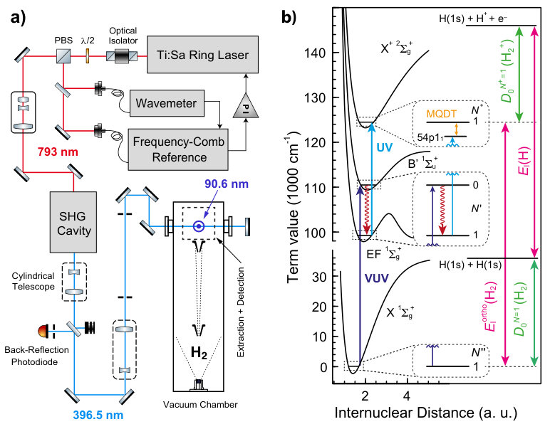 Figure 1
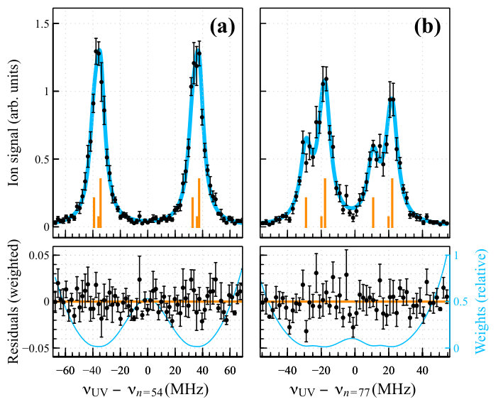 Figure 2
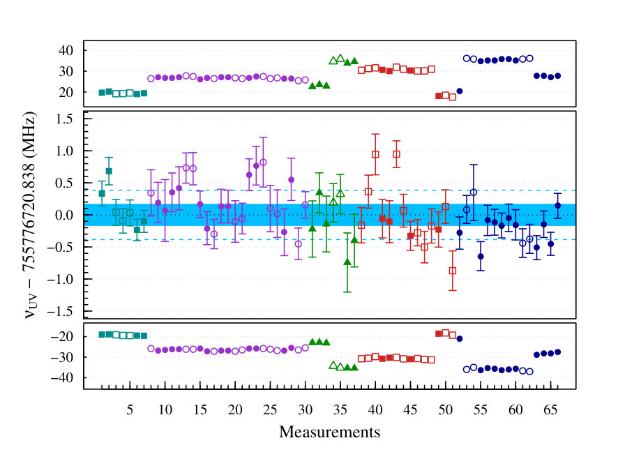 Figure 3
| Transition | ||
|---|---|---|
| Measured frequency | 755 776 720.84(18) MHz | |
| Correction | Uncertainty | |
| DC Stark shift | 10 kHz | |
| AC Stark shift | 5 kHz | |
| Zeeman shift | 10 kHz | |
| Pressure shift | 1 kHz | |
| 1st-order Doppler shift | 200 kHz | |
| 2nd-order Doppler shift | +8 kHz | 1 kHz |
| Line-shape model | 100 kHz | |
| Hfs of EF(0,1) | 100 kHz 333Estimated by multichannel quantum-defect theory in calculations of the type described in Ref. Osterwalder et al. (2004) | |
| Photon-recoil shift | -634 kHz | |
| Systematic uncertainty | 250 kHz | |
| Final frequency | 755 776 720.21(18) | |
| Energy level interval | Value (cm-1) | Uncertainty | Reference | |
|---|---|---|---|---|
| (1) | EF – X | (73 kHz) | Altmann et al. (2018)444Note that the first two columns of Table II of reference Altmann et al. (2018) unfortunately contain errors. The listed intervals in the first column add up to the ionization energy of ortho-H2 instead of the dissociation energy of para-H2, and the values given in the second column of the same table for the binding energy of the 54p11 Rydberg state and the dissociation energy of para-H2 must be corrected to 37.509013(10) cm-1 and 36 118.069 62(37) cm-1, respectively. | |
| (2) | 54p – EF | (300 kHz) | ||
| (3) | X – 54p | (150 kHz) | Sprecher et al. (2014) | |
| (4) | (H2) = (1)+(2)+(3) | (340 kHz) | ||
| (5) | (H) | (18 kHz) | Korobov et al. (2017) | |
| (6) | X – X | (25 Hz) | Korobov (2018) | |
| (7) | (H) = (5)-(6) | (18 kHz) | ||
| (8) | (H) | (3 kHz) | Mohr et al. (2016) | |
| (9) | (H2) = (4)+(7)-(8) | (340 kHz) |
Peer Reviews
No public reviews on file for this paper yet. If you reviewed it on a platform where reviews are public (OpenReview, ICLR, NeurIPS, ICML), you can paste yours below so the community can read it here.
Videos
No videos yet. Explain this paper in a talk, walkthrough, or lecture? Add one.
Benchmarking theory with an improved measurement of the ionization and dissociation energies of H2
Nicolas Hölsch1, Maximilian Beyer1111Present address: Department of Physics, Yale University, New Haven, CT 06511, USA, Edcel J. Salumbides2, Kjeld S. E. Eikema2, Wim Ubachs2, Christian Jungen3 and Frédéric Merkt1,2222Corresponding author; [email protected]
1 Laboratorium für Physikalische Chemie, ETH-Zürich, 8093 Zürich, Switzerland
2 LaserLaB, Department of Physics and Astronomy, Vrije Universiteit, De Boelelaan 1081, 1081 HV Amsterdam, The Netherlands
3 Department of Physics and Astronomy, University College London, UK
(March 17, 2024)
Abstract
The dissociation energy of H2 represents a benchmark quantity to test the accuracy of first-principles calculations. We present a new measurement of the energy interval between the EF state and the 54p11 Rydberg state of H2. When combined with previously determined intervals, this new measurement leads to an improved value of the dissociation energy of ortho-H2 that has, for the first time, reached a level of uncertainty that is three times smaller than the contribution of about 1 MHz resulting from the finite size of the proton. The new result of 35 999.582 834(11) cm*-1* is in remarkable agreement with the theoretical result of 35 999.582 820(26) cm*-1* obtained in calculations including high-order relativistic and quantum electrodynamics corrections, as reported in the companion article (M. Puchalski, J. Komasa, P. Czachorowski and K. Pachucki, submitted). This agreement resolves a recent discrepancy between experiment and theory that had hindered a possible use of the dissociation energy of H2 in the context of the current controversy on the charge radius of the proton.
The dissociation energy of molecular hydrogen, (H2), has been used as a benchmark quantity for first-principles quantum-mechanical calculations of molecular structure for more than a century. H2 consists of two protons and two electrons and is the simplest molecule displaying all aspects of chemical binding. Whereas early calculations were concerned with explaining the nature of the chemical bond Bohr (1913); Heitler and London (1927); James and Coolidge (1933), the emphasis later shifted towards higher accuracy of the energy-level structure, requiring the consideration of nonadiabatic, relativistic and radiative contributions Kolos and Roothaan (1960); Kołos and Wolniewicz (1963, 1968); Wolniewicz (1995); Bubin and Adamowicz (2003); Piszczatowski et al. (2009); E. Mátyus and M. Reiher (2012); Puchalski et al. (2017).
These theoretical developments were accompanied and regularly challenged by experimental determinations of (H2) Langmuir (1912); Witmer (1926); Beutler (1934); Herzberg and Monfils (1961); Herzberg (1969); Stwalley (1970); Eyler and Melikechi (1993); Liu et al. (2009); Cheng et al. (2018). Periods of agreement between theory and experiment have alternated with periods of disagreement and debate. The reciprocal stimulation of theoretical and experimental work on the determination of (H2) has been a source of innovation. With its ups and downs and the related controversies, it has long reached epistemological significance Primas and Müller-Herold (1984); Stoicheff (2001).
In 2009, the experimental (36 118.0696(4) cm*-1*) and theoretical (36 118.0695(10) cm*-1*) values of (H2) reached unprecedented agreement at the level of the combined uncertainties of 30 MHz Liu et al. (2009); Piszczatowski et al. (2009), apparently validating the treatment of the lowest-order () QED correction and the one-loop term of the correction, including several QED contributions that had not been considered for molecules until then. The insight that (H2) is a sensitive probe of the proton charge radius Komasa et al. (2011); Puchalski et al. (2016) stimulated further work.
On the theoretical side, Pachucki, Komasa and coworkers have improved their calculations based on nonadiabatic perturbation theory Pachucki and Komasa (2014, 2015, 2016); Puchalski et al. (2016, 2017), significantly revised the 2009 result, and came to the unexpected conclusion that the excellent agreement of theoretical predictions with experimental (H2) values reached in 2009 was accidental, because of an underestimation of the contribution of nonadiabatic effects to the relativistic correction (see also Refs. Wang and Yan (2018); Puchalski et al. (2018)). In the companion article, Puchalski et al. report on the theoretical progress, with a determination of the leading relativistic correction using the full nonadiabatic wave function M. Puchalski and J. Komasa and P. Czachorowski and K. Pachucki (2018).
Recent experimental work has focused on the determination of the ionization energy of ortho-H2, from which the dissociation energy of ortho-H2, , is obtained using (see Fig. 1b)
[TABLE]
and the very accurately known values of the ionization energy of the H atom ( Mohr et al. (2016)) and of the dissociation energy of ortho-H, Korobov et al. (2017); Korobov (2018). is itself determined as the sum of energy intervals between the X ground state and a selected low- Rydberg states, between this low- Rydberg state and a selected high- p Rydberg state, and the binding energy of the selected high- Rydberg state (see Ref. Sprecher et al. (2011) for details). In the 2009 determination, the selected low- and high- Rydberg states were the EF and the 54p11 Rydberg state. To check the 2009 experimental result, (H2) was first determined by measuring the energy intervals between the X (0,1) and GK states and between the GK(1,1) state and the 56p11 Rydberg state Cheng et al. (2018), after reevaluation of the binding energy of the p11 Rydberg states Sprecher et al. (2014).
In this Letter, we describe a new determination of through the EF(0,1) state with an absolute accuracy improved by a factor of 30 over the 2009 result. The new measurement is also 2.3 times more accurate than, and fully independent of, the measurement via the GK state mentioned above. The accuracy of the 2009 result was limited by the uncertainties arising from (1) the frequency chirps and spectral bandwidths of the pulsed lasers used to record spectra of the EF(0,1) - X(0,1) and 54p11 - EF(0,1) transitions, (2) ac-Stark shifts affecting the Doppler-free two-photon spectra of the EF(0,1) - X(0,1) transition, (3) dc-Stark shifts of the 54p11 - EF(0,1) transition resulting from ions generated in the measurement volume when preparing the EF(0,1) state by two-photon one-color excitation from the X(0,1) ground state, and (4) by the frequency calibration procedure, which relied on comparison with I2 lines.
These limitations have all been overcome: The effects of frequency chirps and ac-Stark shifts were eliminated by using a two-pulse Ramsey-comb method to determine the frequency of the EF(0,1) - X(0,1) transition Altmann et al. (2018) and by using single-mode continuous-wave (cw) ultraviolet (UV) laser radiation to measure the 54p11 - EF(0,1) transition. When recording spectra of the 54p11 - EF(0,1) transition, the generation of ions was entirely suppressed by preparing the EF(0,1) state through single-photon excitation from the X(0,1) state to the B state, followed by spontaneous emission (SE):
[TABLE]
Finally, the relevant frequencies were all calibrated using frequency combs. The measurement of the X(0,1) - EF(0,1) interval by Ramsey-comb spectroscopy has been reported separately Altmann et al. (2018), and we describe here the measurement of the EF(0,1) - 54p11 interval, from which we derive (H2) with a 30-fold improved accuracy over the 2009 result Liu et al. (2009).
The interval between the EF(0,1) state and the 54p Rydberg state of ortho-H2 was measured using the same molecular-beam apparatus and procedures as described in Ref. Beyer et al. (2018), see Fig. 1a. We refer to this work for details on, e.g., the compensation of the stray electric fields to better than 1 mV/cm and the shielding of external magnetic fields. The measurements were performed in a skimmed, pulsed supersonic beam of pure H2 expanding into vacuum from a cryogenically cooled reservoir.
The pulsed vacuum-ultraviolet (VUV) radiation around 90.6 nm used to excite the ground-state molecules to the B state was produced in a four-wave mixing scheme as outlined in Ref. Beyer et al. (2018). The lifetime of the B state is of the order of 1 ns because of rapid spontaneous emission to the lower-lying EF and X states Astashkevich and Lavrov (2015). The angular-momentum selection rule and Franck-Condon factors ensure that almost all molecules decaying to the EF state populate the rovibrational level. Further excitation from the EF(0,1) state to high- Rydberg states using the cw UV laser was detected by pulsed-field ionization (PFI), as described in Ref. Beyer et al. (2018). The delay between the pulsed VUV radiation and PFI was set to 300 ns, i.e., longer than the lifetime of the EF state (), to ensure that a maximum number of molecules could be excited to Rydberg states.
The cw UV radiation used to perform the excitation from the EF(0,1) level to the high- Rydberg states was generated by frequency-doubling the output of a single-mode (bandwidth kHz) Ti:Sa ring laser in an external enhancement cavity containing an LBO crystal. The fundamental frequency of the Ti:Sa laser was calibrated with a frequency comb (accuracy better than 3 kHz) referenced to a 10-MHz GPS-disciplined Rb oscillator. The UV laser beam crossed both the VUV laser beam and the molecular beam at , was retro-reflected by a mirror, and crossed the H2 sample again. Overlapping the forward and reflected UV-laser beams to better than 0.1 mrad and introducing a small deviation from 90∘ of the angle between UV and H2 beam led to two well-separated Doppler components for each transition, from which the Doppler-free transition frequency could be determined as the average of the two peak centers (see Fig. 2 and corresponding discussion).
A telescope was used to place the focus of the UV beam onto the back-reflecting mirror and so ensure two identical Gaussian beams in the excitation region. The reflection angle was checked by monitoring the reflected beam through a 1-mm-diameter diaphragm located 8 m away from the reflection mirror. Complete realignment of the laser and molecular beams between measurements leads to a statistical uncertainty associated with the residual Doppler shift, instead of a systematic one. However, in the error budget, a systematic uncertainty of 200 kHz was included as upper limit for the effects of systematic misalignments. The cancellation of the first-order Doppler shift was verified independently using different angles (and therefore different Doppler shifts, see Fig. 3) and by measuring the transition frequencies using fast and slow H2 beams produced with the valve kept at room temperature and cooled to 80 K, respectively.
Fig. 2 displays typical spectra of the 54p (a) and 77p (b) transitions of H2. Each transition in Fig. 2 splits into two Doppler components, corresponding to photoexcitation with the forward-propagating and reflected UV laser beams, as explained above. The 54p transition was selected because the binding energy and hyperfine structure (hfs) of the 54p Rydberg states are precisely known from previous studies combining millimeter-wave spectroscopy and multichannel quantum-defect theory (MQDT) Osterwalder et al. (2004); Sprecher et al. (2014). The 77p transition was used as reference and was measured after each realignment to detect possible drifts of the stray fields and of the UV-laser propagation axes with respect to the molecular-beam axis. Because the polarizability of Rydberg states scales as , the 77p state is more than 10 times more sensitive to stray fields than the 54p state, making stray-field drifts of 1 mV/cm easily detectable. Such drifts would shift the frequency of the 54p transition by less than 10 kHz. The hyperfine splittings of the p series become larger with increasing value Sprecher et al. (2014). Consequently, the hfs of the 77p state could be partially resolved, which enabled us to verify experimentally that the intensities of the transitions to the three accessible () components are proportional to . Systematic uncertainties resulting from fits of the lineshapes with our lineshape model could thus be reduced to 100 kHz (see below and Refs. Beyer et al. (2018); Hölsch et al. (2018)).
To determine the line positions, we fitted the lineshape model described in Ref. Beyer et al. (2018), which consists, for each Doppler component, of a superposition of three line profiles corresponding to the three hyperfine components of the p Rydberg states, with intensities proportional to . For the 54p and 77p Rydberg states, we used the hyperfine splittings determined by millimeter-wave spectroscopy Osterwalder et al. (2004) and MQDT calculations, respectively. Voigt profiles with a full width at half maximum of 9 MHz and a Lorentzian contribution of about 6 MHz were found to best reproduce the measured line profiles. The lineshape depends on the velocity distribution in the volume defined by the intersection of the VUV, UV and gas beams Hölsch et al. (2018); Beyer et al. (2018), with contributions from transit-time broadening and Doppler-broadening originating from the photon recoil of the B EF spontaneous emission.
Repeated measurements of these transitions revealed a high sensitivity of their frequencies to the alignment of the forward-propagating and reflected UV laser beams. Misalignments were detectable through an intensity imbalance between the two Doppler components. This effect turned out to be more pronounced than in our previous study of p/f transitions, an observation we attribute to the twice higher frequency of the p transitions and the resulting increased Doppler effect. In the final analysis of the data and after careful calibration of the effects of intentional, well-defined misalignments, we rejected all measurements associated with intensity ratios of the two Doppler components lying outside the range [0.8,1.25], and included a systematic uncertainty of 200 kHz (see above and Table 1).
Table 1 also lists the other sources of systematic uncertainties considered in our analysis, which were estimated as explained in detail in Ref. Beyer et al. (2018), and include uncertainties arising from DC and AC Stark shifts, Zeeman shifts, pressure shifts, Doppler shifts, and two contributions of each 100 kHz to account for uncertainties associated with the line-shape model and the unresolved (and unknown) hfs of the EF(0,1) state. The transitions frequencies were corrected by adding 8 kHz for the second-order Doppler shift and subtracting kHz for the photon-recoil shift, which is more than twice as large as the combined statistical and systematic uncertainty of 300 kHz.
The measurements used to determine the frequency of 54p transition were carried out at a valve temperature of 80 K and are depicted in Fig. 3, which gives the central positions of the upper and lower Doppler components in the top and bottom panels, respectively, and the average (Doppler-free and hyperfine-free) frequency with their statistical uncertainties (1) in the middle panel. The different colors and symbols indicate measurements carried out on different days and the sequence of full and open symbols indicate realignment of the laser beams. The dashed blue lines correspond to the standard deviation of the whole data set and the area shaded in blue the standard deviation of the mean. Adding the corrections listed in Table 1 and combining all uncertainties in quadrature yields the value of 755 776 720.21(30) MHz (25 209.997 785(10) cm*-1*) for the 54p interval.
Table 2 provides the details of the determination of the ionization and dissociation energies of H2 from the three intervals (entries (1), (2) and (3) in the table) linking the X(0,1) and X+(0,1) ground states of ortho-H2 and H and corresponding to a value of of 124 357.238 003(11) cm*-1*. A value of 35 999.582 834(11) cm*-1* can be derived for using Eq. (1). The error budget in Table 1 also applies to the 77p transition, with the exception of the uncertainty resulting from the dc Stark shift (100 kHz). A determination of using the binding energy of the 77 state is in agreement with the results given in Table 2, proving the internal consistency of the MQDT analysis presented in Ref. Sprecher et al. (2014).
Because of the very accurate value of the X-EF interval, our new result is more precise than the result of the measurement through the GK(0,1) state (35 999.582 894(25) cm*-1* Cheng et al. (2018)), from which it differs by about . It is in agreement with the theoretical result (35 999.582 820(26) cm*-1*) obtained by Puchalski et al. (see companion article M. Puchalski and J. Komasa and P. Czachorowski and K. Pachucki (2018)). This agreement between experiment and theory at the accuracy level of better than 1 MHz resolves the discrepancy noted in recent work Puchalski et al. (2017) and may be regarded as unprecedented in molecular physics. The error margins within which theoretical and experimental values of (H2) agree are 30 times more stringent than in 2009. This agreement opens up the prospect of using (H2) to make a contribution to the solution of the proton-radius puzzle Pohl et al. (2010) as well as in the search or exclusion of fifth forces (see discussion in Ref. Salumbides et al. (2013)). The experimental uncertainty of 340 kHz of the present result represents 30% of the expected total contribution of 1 MHz to from the finite size of the proton Puchalski et al. (2016). The main sources of uncertainty of the present result come from the (unresolved) hfs of the EF(0,1) level, which affects both the X(0,1)-EF(0,1) and the EF(0,1) - 54p intervals and uncertainties associated with the residual first-order Doppler shift and the line shape model (see Table 1). These sources of uncertainties would be significantly reduced in a measurement in para-H2, which should be the object of future efforts. In this context, theoretical work should consider the ionization energy of H2 (see also M. Puchalski and J. Komasa and P. Czachorowski and K. Pachucki (2018)), which is the quantity we directly measure and which we obtain experimentally with a relative accuracy () of .
Acknowledgements.
FM, WU and KE acknowledge the European Research Council for ERC-Advanced grants under the European Union’s Horizon 2020 research and innovation programme (grant agreements No 670168, No 743121 and No 695677). KE and WU acknowledge FOM/NWO for a program grant (16MYSTP). FM acknowledges the Swiss National Science Foundation (grant 200020-172620).
The reference list from the paper itself. Each links out to its DOI / PubMed record.
- 1Bohr (1913) N. Bohr, Phil. Mag. 26 , 857 (1913).
- 2Heitler and London (1927) W. Heitler and F. London, Z. Phys. 44 , 455 (1927).
- 3James and Coolidge (1933) H. M. James and A. S. Coolidge, J. Chem. Phys. 1 , 825 (1933), see correction in J. Chem. Phys. 3, 129 (1935).
- 4Kolos and Roothaan (1960) W. Kolos and C. C. J. Roothaan, Rev. Mod. Phys. 32 , 219 (1960).
- 5Kołos and Wolniewicz (1963) W. Kołos and L. Wolniewicz, Rev. Mod. Phys. 35 , 473 (1963).
- 6Kołos and Wolniewicz (1968) W. Kołos and L. Wolniewicz, Phys. Rev. Lett. 20 , 243 (1968).
- 7Wolniewicz (1995) L. Wolniewicz, J. Chem. Phys. 103 , 1792 (1995).
- 8Bubin and Adamowicz (2003) S. Bubin and L. Adamowicz, J. Chem. Phys. 118 , 3079 (2003).