Radiative transport of relativistic species in cosmology
Cyril Pitrou

TL;DR
This paper reviews the construction of distribution functions for fermions and photons in cosmology, emphasizing their similarities and differences, and introduces methods to handle polarization, anisotropy, and spectral distortions in the Boltzmann equations.
Contribution
It provides a unified framework for fermion and photon distribution functions, including polarization and anisotropy, and extends the Kompaneets equation to more general cases.
Findings
Unified treatment of fermion and photon distribution functions.
Extension of the Kompaneets equation to anisotropic and polarized photons.
Parameterization of photon spectra using logarithmic moments.
Abstract
We review the general construction of distribution functions for gases of fermions and bosons (photons), emphasizing the similarities and differences between both cases. The central object which describes polarization for photons is a tensor-valued distribution function, whereas for fermions it is a vector-valued one. The collision terms of Boltzmann equations for fermions and bosons also possess the same general structure and differ only in the quantum effects associated with the final state of the reactions described. In particular, neutron-proton conversions in the early universe, which set the primordial Helium abundance, enjoy many similarities with Compton scattering which shapes the cosmic microwave background and we show that both can be handled with a Fokker-Planck type expansion. For neutron-proton conversions, this allows to obtain the finite nucleon mass corrections,…
Click any figure to enlarge with its caption.
 Figure 1
 Figure 2
 Figure 3
 Figure 4
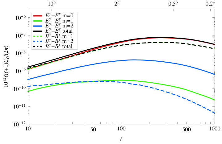 Figure 5
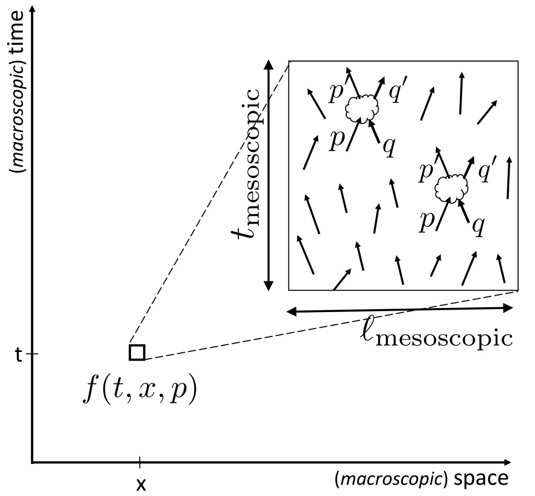 Figure 6
 Figure 7
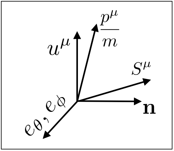 Figure 8
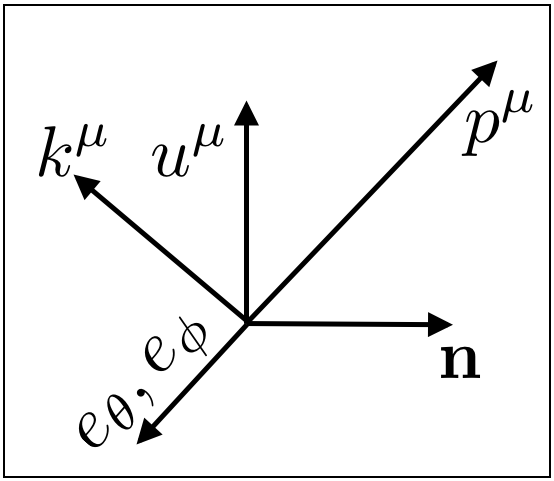 Figure 9
| Reaction | Particles names | Chiral couplings | |
|---|---|---|---|
Peer Reviews
No public reviews on file for this paper yet. If you reviewed it on a platform where reviews are public (OpenReview, ICLR, NeurIPS, ICML), you can paste yours below so the community can read it here.
Videos
No videos yet. Explain this paper in a talk, walkthrough, or lecture? Add one.
Radiative transport of relativistic species in cosmology
Cyril Pitrou
Institut d’Astrophysique de Paris, CNRS UMR 7095,
Institut Lagrange de Paris, 98 bis Bd Arago 75014 Paris, France
Abstract
We review the general construction of distribution functions for gases of fermions and bosons (photons), emphasizing the similarities and differences between both cases. The central object which describes polarization for photons is a tensor-valued distribution function, whereas for fermions it is a vector-valued one. The collision terms of Boltzmann equations for fermions and bosons also possess the same general structure and differ only in the quantum effects associated with the final state of the reactions described. In particular, neutron-proton conversions in the early universe, which set the primordial Helium abundance, enjoy many similarities with Compton scattering which shapes the cosmic microwave background and we show that both can be handled with a Fokker-Planck type expansion. For neutron-proton conversions, this allows to obtain the finite nucleon mass corrections, required for precise theoretical predictions, whereas for Compton scattering it leads to the thermal and recoil effects which enter the Kompaneets equation. We generalize the latter to the general case of anisotropic and polarized photon distribution functions. Finally we discuss a parameterization of the photon spectrum based on logarithmic moments which allows for a neat separation between temperature shifts and spectral distortions.
Contents
Introduction
We review theoretical and practical aspects of the radiative transport of relativistic species. Our emphasis is on cosmological applications, hence we focus on fermions (neutrons, protons, electrons, positrons and neutrinos) during big-bang nucleosynthesis (BBN) and photons of the cosmic microwave background (CMB). Relativistic species cannot be described by perfect fluids and one must account for the distribution of particles using a distribution function , whose evolution is dictated by a Boltzmann equation . The left hand side is the Liouville term and describes the free streaming of particles. In a curved space-time, this requires the use of cosmological perturbation theory, that is general relativity. The emphasis of this article is on the right hand side which is the collision term, and describes the evolution of the distributions under the influence of collisions, that is because of the micro-physics. Hence all the results presented here are independent of any perturbation theory, as they are derived from the basic principles of particle physics. From the equivalence principle, they are formulated in a local orthonormal frame, that is in the context of special relativity.
It is instructive to consider the cases of fermions and bosons side by side as their description by distribution functions have numerous similarities. In fact, the case of massless fermions is simpler than the case of photons in many respects, essentially because the spin of fermions () is smaller than the spin of photons (). Hence the paper is organized to allow for a detailed comparison of these two cases. We show that the collision term for weak interactions during BBN has a structure which is extremely similar to the structure of the collision term for photons due to Compton scattering. Furthermore, we can use common techniques to express in practice these collision terms in functions of the distribution functions moments. Even though one could follow the analogy for anisotropic distribution functions, it is not useful for the case of fermions in the context of BBN. Hence we study in details the angular structure only for Compton scattering and derive the extended Kompaneets equation, valid for anisotropic and polarized photon distributions. Since the emphasis is on the derivation and the structure of the equations, we only summarize how the equations must be applied in the cosmological context, overviewing briefly the main physical effects.
In § I a general procedure to build a classical distribution function out of the quantum number operator is summarized. We then detail in § II how a classical Boltzmann equation can be derived, given a set of suitable approximation and assumptions, from the quantum evolution of the number operator. Sections III is then dedicated to the collision terms of weak interactions processes for fermions in the early universe. In order to compute in practice these collision terms, we review the Fokker-Planck expansion in § IV applied to BBN weak interactions. The similar treatment of Compton interactions between electrons and photons and its Fokker-Planck expansion are reviewed in § V. Applications for the evolution of isotropic photon distributions under Compton interactions are presented in § VI, with a brief discussion on its implications for cosmology. The detailed form of the collision term for anisotropic distributions, including polarization is subsequently exposed in § VII, using symmetric trace-free tensors to decompose the angular dependence. It is the first general derivation of the Compton collision term in the literature which includes thermal and recoil effects while describing consistently polarization. Finally we present in § VIII a parameterization for spectral distortions and we collect in § IX the equations governing the generation of distortions from the Thomson part of the collision term, with plots of the associated angular power spectrum generated during the reionization era.
Theoretical framework
I Distribution functions
In this section, based on Fidler and Pitrou (2017), we review how the distribution function is built from the quantum expectations of the number operator, and how its covariant components can be extracted. We also show that for each spin there is an adapted expansion in spin-weighted spherical harmonics for the dependence on the spatial momentum direction. The case of fermions is presented first, even though it is less known, as it allows to understand better the photon case.
I.1 General construction
I.1.1 Notation
Before considering the kinetic theory in curved spacetime, we build the formalism in a flat space-time (that is the Minkowski space-time of special relativity) in which the quantum theory of particles is very well established. An inertial frame is defined by a tetrad field, that is by a timelike vector field and three spacelike vector fields , together with the associated co-tetrad . Latin indices such as indicate spatial components in the tetrad basis. A four-vector is written as where Greek indices denote components in the tetrad basis. In particular, the components of the tetrad vectors and co-vectors in the tetrad basis are by definition and . If gravity can be ignored, that is in the context of special relativity, the inertial frame is global. Later, when including the effect of gravity in the context of general relativity, the inertial frame is local and one must employ general coordinates whose indices are labelled by . For a given vector this implies .
The momentum vector will often simply be denoted as and its spatial components allow to build the spatial momentum . More generally, we reserve boldface notation to spatial vectors. The energy associated with the momentum is given by the time component
[TABLE]
When a quantity depends on the spatial momentum, we use indifferently or when no ambiguity can arise. The (special) relativistic (and Lorentz covariant) integration measure is defined as
[TABLE]
and its associated (special) relativistic Dirac function is defined accordingly as
[TABLE]
such that . Our metric convention follows the standard notation employed in cosmology, which is the opposite of the metric commonly used in particle physics. In the tetrad basis, the metric reduces to the Minkowski metric
[TABLE]
The Levi-Civita tensor is fully antisymmetric and in the tetrad basis all its components are deduced from the choice
[TABLE]
We identify the time-like vector of a tetrad with the velocity of an observer and its spatial Levi-Civita tensor is obtained from , such that .
I.1.2 Number operator
Creation and annihilation operators, and respectively, where the index refers to a helicity basis and to the particle momentum, are defined for each particle type from its corresponding quantum field. It allows to define a quantum number operator as
[TABLE]
The total occupation operator is then obtained from a sum over all possible momenta of the diagonal part as
[TABLE]
When considering a given quantum state , the average of the number operators allows to define a distribution function with helicity indices as
[TABLE]
Hence the total number of particles is given by
[TABLE]
where we introduced the total volume . In this expression, corresponds exactly to the definition of a classical one-particle distribution function. By construction and are Hermitian, that is
[TABLE]
So far we have not specialized to particles nor antiparticles, not even to a special spin type (fermions or bosons), and this construction is very general. In the next two sections we study separately fermions and bosons, and we show how the distribution function with helicity indices () can be decomposed into covariant components.
I.1.3 Adapted orthonormal basis
For a given observer with four-velocity which is chosen to be aligned with the time-like tetrad vector , we define the unit spatial vector of momentum direction by
[TABLE]
In spherical coordinates the momentum direction is given by and defines a radial unit vector. We then also consider the usual basis in spherical coordinates and , which are purely spatial unit vectors. In tetrad components these are given by
[TABLE]
Let us introduce the helicity vector
[TABLE]
which is a unit vector in the direction of the spatial momentum that is transverse to in the sense , and is thus spacelike. Since the space of vectors orthogonal to is three-dimensional, the transverse property is not enough to specify the helicity vector and the definition (23) depends explicitly on the observer which is used to define the spatial part of the momentum. When no ambiguity can arise we write simply . In components the helicity vector is given by
[TABLE]
Geometrically (see Fig. 1), the helicity vector corresponds to the spatial direction unit vector boosted in its direction by the same boost needed to obtain from .
Finally, we define the polarization basis
[TABLE]
where again the dependence on can be omitted whenever no ambiguity can arise.
The set of vectors , and constitute an adapted orthonormal basis to a given observer and a given momentum.
I.1.4 Fermions
The quantum fermion field is
[TABLE]
and satisfies the Dirac equation . In this expression, the creation and annihilation operators of the particles () and antiparticles () satisfy the anti-commutation rules
[TABLE]
with all other anti-commutators vanishing and where is the Kronecker function.
We then define the operator in spinor space (beware of position of helicity indices for antiparticles)
[TABLE]
For the sake of clarity we use a notation where components of operators in spinor space and Dirac spinors are explicit and are denoted by indices of the type . The plane waves solutions and are the positive and negative frequency solutions and satisfy
[TABLE]
with the standard Dirac slashed notation and the Dirac matrices satisfying the algebra . As detailed in appendix A, all spinor space operators can be decomposed on the complete set
[TABLE]
and in particular the operators (31) are decomposed as
[TABLE]
Note also how the indices are in reverse order for antiparticles ( instead of ) echoing a similar placement of indices in Eqs. (31).
The operators of the type (309) take a simple form in the adapted orthonormal basis defined in § I.1.3. Using the helicity basis
[TABLE]
where the right and left chiral parts are defined as
[TABLE]
we obtain
[TABLE]
In particular, we recover when summing on helicities the standard result
[TABLE]
Furthermore, when helicities are different, we obtain the so-called Bouchiat-Michel formulae (Bouchiat and Michel, 1958) [see also Dreiner et al. (2010, App. H.4) or Langenfeld (2007, App. E.3)]. Using the polarization basis (25) we show (Fidler and Pitrou, 2017, App. D7) that it is cast in the compact form
[TABLE]
Let us define111We use the obvious abuse of notation for e.g. . from the distribution function with helicity indices
[TABLE]
together with
[TABLE]
The functions are the Stokes parameters. In detail, is the total intensity, the circular polarization, and is the purely linear polarization vector. is the total polarization vector, taking into account both circular and linear polarization. By construction the total polarization is transverse to the momentum (). The linear polarization is transverse both to the momentum and to the observer velocity , that is it is a purely spatial vector.
The covariant parts are defined from the decomposition
[TABLE]
[TABLE]
One degree of freedom corresponds to the total intensity while the three remaining degrees correspond to the state of polarization and are covariantly contained in a vector because of its transverse property.
The decomposition (45) can be understood from group representations. Indeed, the total polarization vector is a spin- representation of and the intensity is a spin-[math] representation. When forming the number operator (6), and thus , we are building the tensor product of spin- representations and what we have achieved is a decomposition of the reducible representation in irreducible components , where we have denoted the spin- representations of .
I.1.5 Massless fermions
In the massless limit, the previous decomposition is slightly modified to
[TABLE]
with defined in Eq. (305). Note that the linear polarization and the circular polarization enter separately, and not as a total polarization vector as is the case for massive fermions. Using it can also be rewritten as
[TABLE]
In the massless case, the little group of the Lorentz group (Weinberg, 1995) is not but . Hence the decomposition in irreducible representations is of the form where the purely linear polarization is in the spin- representation of (noted ) and circular polarization is in the representation .
Also, it is no longer possible to overtake the particles as they move at the speed of light in any coordinate system. This leads to both, the circular and linear polarizations and to be individually observer independent. More rigorously, linear polarization is described by the coset of
[TABLE]
Indeed, since the polarization basis satisfies , but we also have , there is a gauge freedom in the definition of the polarization basis. The choice (25) corresponds to the particular choice which is also transverse to the observer velocity (), which selects unique representatives of polarization vectors. Therefore the polarization vector representative are observer dependent, but not the associated cosets . As a consequence is observer dependent but not its coset .
Given a representative of the coset, the one associated with a given observer (that is such that it is transverse to that observer velocity) is obtained by projection with a screen projector , which is abbreviated as when no ambiguity can arise. Using the decomposition of the null momentum into energy and unit direction
[TABLE]
where , the screen projector is built from the equivalent definitions
[TABLE]
with is a future directed null vector in the plane spanned by such that , . It can be checked that the screen projector satisfies the expected properties and . If the observer used in the definition is the natural observer associated with the tetrad with which components are taken (that is if ), the non-vanishing components of the screen projector are only .
For two screen projectors associated with two observers and related by a boost
[TABLE]
but for the same momentum , we find that they are related by
[TABLE]
where . In particular this implies
[TABLE]
Using the screen projector, another definition of the linear polarization coset is that two polarization vectors and describe the same state () if
[TABLE]
Note that for a transverse vector () it is obvious from the decomposition (51) or the transformation rule (53) that
[TABLE]
implying that the definition (55) is unambiguous.
For photons, that is massless bosons, on which we focus in the next section, the structure is exactly similar and arises from the electromagnetic gauge freedom.
I.1.6 Massless bosons
The null mass bosonic vector field of quantum electrodynamics is
[TABLE]
where the creation and annihilation operators satisfy the commutation rule
[TABLE]
If vectors are massive, then the null helicity () must also be considered, see Fidler and Pitrou (2017, App. A).
A covariant distribution tensor is obtained by considering
[TABLE]
and by construction it is transverse to the momentum and the observer’s velocity (). When no ambiguity can arise, we omit the dependence on the observer’s velocity used in its definition.
We define
[TABLE]
as the usual Stokes parameters222It is sometimes customary in the cosmic microwave background context to define the distribution function as Durrer (2008) . Accordingly, the tensor valued function (58) is defined as . With this definition the Stokes parameters are , and . corresponding to intensity, circular polarization and linear polarization. For a given observer with four-velocity , we use as in the massless fermion case the spatial momentum direction unit vector defined in the decomposition (50). Let us also define the two-dimensional Levi-Civita tensor
[TABLE]
We usually omit the dependence on and write simply . The tensor-valued distribution function is decomposed as
[TABLE]
where the screen projector is defined exactly as for massless fermions in Eqs. (51). The distribution tensor is doubly transverse, that is transverse to the momentum and also to the observer velocity . is the linear polarization tensor and it is doubly transverse and traceless (it satisfies ). It is defined as
[TABLE]
and its dependence on is often omitted. It can be extracted thanks to the transverse traceless projector
[TABLE]
In the basis the components of the distribution tensor (61) form a Hermitian matrix Hu and White (1997); Tsagas et al. (2008); Durrer (2008)
[TABLE]
whereas in the basis we obtain the Hermitian matrix
[TABLE]
For massless bosons, the structure of the decomposition can also be understood exactly like in the discussion following Eq. (48) for massless fermions. The difference is that for massless bosons, we decompose into , where (resp. ) is the spin- (resp. spin-) representation of .
As in the case of massless fermions, the definition (58) and the decomposition (61) of the distribution tensor is observer dependent, for exactly the same reasons that the polarization vectors are defined up to factors of . Hence, we should rather consider the coset . Two polarization states and are in the same coset if
[TABLE]
In particular, the linear polarization parts and are equivalent if
[TABLE]
and one should rather consider the coset of linear polarization. With arguments similar to Eq. (56), this definition of equivalence (and its associated cosets) is observer independent.
I.2 Multipolar decomposition
I.2.1 Fermions
The intensity is easily decomposed into spherical harmonics. Indeed, once an observer choice is made, that is its four-velocity is identified with the time-like vector of the tetrad , we can define the spatial momentum and its direction unit vector (see § I.1.3). We then perform the usual spherical harmonics decomposition
[TABLE]
Using Eq. (325) the multipoles are extracted as .
Alternatively one could use a decomposition based on symmetric trace-free (STF) tensors which is equivalent Thorne (1980); Blanchet and Damour (1986); Pitrou (2009a, b)
[TABLE]
where we use the tools and notation summarized in appendix D. From Eq. (325) the STF tensors are extracted as
[TABLE]
The relation between both expansions is obtained from Eqs. (D.2) as
[TABLE]
For the polarization vector of fermions defined in Eq. (44), we have to pay attention to the transformation properties when performing a spatial rotation of the coordinate system around the direction of . The ordinary spherical harmonics, when evaluated at do not transform under this rotation and are thus not suitable to decompose objects which have a non-trivial transformation under this rotation. The polarization vector transforms as an ordinary 4-vector (we have shown that it is observer-independent). However, this is not the case for the observer-dependent vectors and distribution functions used to build . The vector in direction of the spatial momentum is invariant under this particular rotation as it points in the direction . Employing the observer-independence of which is discussed in the next section, we therefore conclude that must be invariant under this rotation and may be decomposed into ordinary spherical harmonics.
[TABLE]
Again an expansion in STF tensors of the type (69) is possible and is obtained by relations exactly similar to Eqs. (71).
The polarization vectors however transform with an additional spin complex rotation. To generate an observer-independent the corresponding must transform with the opposite spin and they are decomposed into spin-weighted spherical harmonics Goldberg et al. (1967) as
[TABLE]
Note that this discussion only concerns the observer dependence under a specific spatial rotation and that due to the definition of helicity an additional dependence mixing and exists for more general rotations and boosts. and modes multipoles can be defined from
[TABLE]
The have even parity (they get a factor under parity transformation) whereas the have odd parity (they get a factor under parity transformation) since spin-weighted spherical harmonics transform as and the polarization basis transforms as . Equivalently since is a vector field on the unit sphere in momentum space, it can be decomposed as the gradient and the curl of two scalar functions as
[TABLE]
where is the covariant derivative on the unit sphere and is the Levi-Civita tensor on the unit sphere already defined in Eq. (60). Decomposing the scalar functions and in multipoles and as in the expansion (68) and using Durrer (2008)
[TABLE]
the two possible definitions for the and modes multipoles are related by and . Again a similar expansion can be obtained by using symmetric trace-free tensors to expand the scalar functions and directly in Eq. (75).
I.2.2 Massless bosons
The decomposition of intensity and circular polarization is performed with spherical harmonics as in Eqs. (68) and (72) or with STF tensors as detailed in § I.2.1 for fermions. However, the linear polarization part must be decomposed in spin- spherical harmonics. We decompose polarization as
[TABLE]
and the angular decomposition is
[TABLE]
Note that the factor in Eq. (77) is purely conventional. and modes are defined by
[TABLE]
Equivalently linear polarization can be decomposed with two potentials on the unit sphere in momentum space as (Tsagas et al., 2008, Eq. 4.3.8)
[TABLE]
and the associated multipoles and can be related to the and by some factors. Instead, if we use an expansion of and in STF tensors of the type (69), we can decompose with them. However, it is customary to remove the factors brought by the covariant derivatives and use the expansion (Dautcourt and Rose, 1978) [see also Tsagas et al. (2008, Eq. 4.3.9) or Pitrou (2009a, Eq. 1.33)]
[TABLE]
The exponent indicates that free indices are to be projected on the transverse traceless part with the operator (63). From the definition (77) of , and using the notation (337), this expansion is equivalent to
[TABLE]
The STF tensors of the decomposition (81) are extracted thanks to (Tsagas et al., 2008; Pitrou, 2009a)
[TABLE]
where
[TABLE]
If we now associate to these STF tensors and the and , using a relation of the type (71), these are related to the and defined in (79) by
[TABLE]
This is obtained using Eqs. (340) in Eq. (82) and comparing with Eq. (78).
I.3 Observer independence
In this section, we detail the transformation property of the distribution function under a general Lorentz transformation . It is more appropriate to take the passive point of view and consider a transformed tetrad basis related to the initial one by
[TABLE]
The new observer’s velocity is identified with the time-like vector of the new tetrad . That is we take the point of view that when considering a change of frame we also consider the associated change of observer, such a that any observer is not moving in its own frame. In that sense, the observer’s velocity is not observer independent.
The new components of the momentum are related to the previous ones by
[TABLE]
and we abbreviate as .
I.3.1 Massive fermions
In Fidler and Pitrou (2017), we showed that the spinor valued operator transforms under the Lorentz transformation defined by Eqs. (86) as
[TABLE]
where is the spinor-space representation of . Using the property for Dirac matrices
[TABLE]
it implies that the covariant components for massive fermions transform as
[TABLE]
This means that they transform exactly as a scalar and vector field, and they are therefore observer independent.
The observer independence is important as it allows to build a statistical description of the fluid without the need to specify an observer first. This is particularly useful for deriving simple transport equations in general relativity.
The scalar describes the total intensity of the field and is observer independent since the local number of particles is identical for each observer. The information of the polarization of the fluid is contained in the observer independent vector .
On the other hand the parameters and , describing individually the circular and linear polarizations are not observer independent. The circular polarization , for example, changes if the observer is boosted and overtakes the momentum considered. We have defined
[TABLE]
where combines multiple observer dependent quantities into one observer independent vector. In the example of the observer overtaking a particle momentum, we change all left-helical states into right-helical states. This means that the boosted observer will find . At the same time the vector is also observer dependent and the new observer will define the spatial momentum of the particles with the opposite sign. Therefore the combination is invariant under this boost. At the same time the off-diagonal distributions are swapped: . However these are combined with the polarization vectors to form , which are also interchanged for the new observer, leading to being invariant.
In a more general case and cannot be disentangled in an observer independent manner and there always exists a subset of observers, all related by boosts along the momentum direction and rotations around the momentum direction, that will perceive the field to be entirely circularly polarised without any linear polarization. For this reason we will work with the observer independent polarization vector and only refer to the circular and linear polarizations when we have specified an observer. Only in the case of massless fermions, considered in § (I.1.5), the linear and circular polarization can be disentangled, and are observer independent, the latter in the sense of the polarization coset (49) as detailed in the next section.
I.3.2 Massless fermions
Using the decomposition (47) for massless fermions, we deduce that the covariant components transform as
[TABLE]
The screen projector [see Def. (51)] associated with the new observer and the new momentum components,
[TABLE]
(with ) ensures that the linear polarization remains spatial for the new observer. Hence in the massless case, the linear polarization part is not strictly observer independent, but since this dependence introduced by the screen projector is there only as the result of a choice to remove a non physical degree of freedom, we can still conclude that in that sense the covariant components are observer independent. More rigorously, it is the coset of linear polarization [see definition (49)] which is observer independent and only the special choice of its representative element is observer dependent. Hence we should rather write the transformation rule of linear polarization cosets which is
[TABLE]
for which the observer independence is manifest.
I.3.3 Massless bosons
For massless bosons, the tensor-valued distribution function transforms as
[TABLE]
with the definition . Since the screen projector satisfies333This is exactly Eq. (53) but expressed with components associated to different tetrads.
[TABLE]
and the two-dimensional Levi-Civita tensor (60) satisfies a similar property, then we deduce that the covariant components transform as
[TABLE]
where is the transverse-traceless projector associated with , using the definitions (63) and (93). As in the case of massless fermions, it is the coset of linear polarization [see Eq. (66)] which is observer independent, and only the special choice of its representative element is observer dependent. Hence we should rather write the transformation rule as , with the cosets defined by the equivalence relation (66), and for which the observer independence is manifest.
I.3.4 Relation to abstract tensor indices
Since we have shown that all components of the vectors or tensors associated to fermions and photons have the expected transformation properties, we could decide to work with abstract indices as in Challinor et al. (2000); Challinor (2000a); Tsagas et al. (2008) instead of working with indices referring to a particular tetrad. In most cases this reinterpretation is straightforward. However both approaches differ when it comes to expressing in practice the transformation of the STF tensors presented in § I.2 for the angular decomposition of the distribution functions. With abstract indices, projectors still appear in the transformation rules, as e.g. in Eqs. (4.3.31-4.3.33) of Tsagas et al. (2008), whereas with indices referring to components in tetrads the transformations relate STF tensors which all are purely spatial in their associated tetrad, that is we relate only spatial indices, as in Eqs. (1.56-1.58) of Pitrou (2009a). However, this subtlety only shows when the transformation of the multipoles is performed at least at second order in the boost velocity. In the remainder of this article, we use a method where no change of frame is needed, hence we do not detail any further the procedure to obtain the multipoles transformation rules. More details can be found in Pitrou (2009a).
II Boltzmann equation
II.1 Liouville equation in curved space-time
The previous construction was restricted to a homogeneous system, hence the functions appearing ( and ) depended only on . In order to describe a gas of particles classically, one must assume that this construction is in fact valid only locally. That is we assume that there is a mesoscopic scale and that our previous construction was restricted to scales much smaller. The functions, which were dependent on must depend now on . In order to derive a Liouville equation in curved space-time which describes the evolution of the covariant components, we must also distinguish between the massive and the massless cases.
II.1.1 Massive fermions
In the previous sections we have shown that and are observer independent. In addition, in the local Minkowski frame, they are also parallel transported in the absence of collisions. The helicity of particles does not change in free propagation and, considering that the momentum is conserved, the vectors and used to build the quantities and remain unchanged. Hence, in the local Minkowski space we obtain the equations of motion
[TABLE]
From the point of view of general relativity, these equations are only valid locally and neglect entirely the impact of the relativistic space-time. The intensity describes the total number of particles. The conservation of in the absence of collisions in Eq. (98) is equivalent to mass or particle number conservation. The geometrical impact of general relativity does not change the number of particles and we may generalise the equation of motion by requiring the conservation of along a full geodesic
[TABLE]
where is the derivative along the particle trajectory parameterized by .
The vector is parallel transported in the local space-time and describes the polarization of particles in an observer-independent way. Again, the geometrical nature of general relativity does not change the polarization of particles and we require that is parallel transported along the non-trivial trajectory of the particles. Note that the observer dependent linear and circular polarization may change non-trivially during the transport and require a specification of the dynamics of the observer.
Using the observer-independence, we are able to uniquely define the vector on our full space-time by employing the tetrads
[TABLE]
where we remind that the index is a tetrad component index, but the index is a general coordinate index. Assuming parallel transport, we obtain the equation of motion
[TABLE]
Note that is by definition orthogonal to the momentum. This property is automatically conserved in the relativistic evolution as both the momentum and are parallel-transported along the geodesic of a free particle.
II.1.2 Massless fermions
In the massless case, linear polarization and circular polarization must be considered separately. Circular polarization is transported exactly like the intensity in Eqs. (99) because the direction of the helicity vector is identical to the momentum and therefore parallel-transported. However the linear polarization vector (considered in general coordinates with ) cannot be parallel transported because it is transverse to both the momentum and the observer velocity , and the latter is not (necessarily) parallel transported. However, in the process of free streaming, any variation of in the direction of the momentum is not physical. Hence this unphysical degree of freedom must be eliminated by an appropriate projection so as to obtain an unambiguous equation for parallel transport. To that purpose, we use the screen projector (51) in general coordinates and write
[TABLE]
The transport of linear polarization in the massless case is the same as the transport of the full polarization vector in the massive case [Eq. (101)], up to an additional screen projection which ensures that the double transverse property holds. It can be equivalently formulated by saying that the coset is parallel transported, that is
[TABLE]
II.1.3 Massless bosons
The parallel transport of linear polarization for massless bosons, that is photons is very similar to massless fermions, except that instead of projecting a vector we must project a tensor (Challinor, 2000b, a; Tsagas et al., 2008; Pitrou, 2009a, b). We define polarization on the full spacetime as in Eq. (100), that is
[TABLE]
Similarly, the non-physical degree of freedom must be projected and the evolution of linear polarization is dictated by
[TABLE]
Note that for massless bosons, we need not postulate this equation as it is obtained from the eikonal approximation of electromagnetism, see e.g. Fleury (2015) for a detailed account on the procedure.
II.2 Quantum evolution in the interaction picture
So far we have discussed the free propagation of fermions or bosons. When in addition considering collisions, we will employ a separation of scales. We assume that the relativistic evolution is dominant on macroscopic scales, while individual collisions act on microscopic scales. We therefore may compute the collision term in the local tangent space corresponding to special relativity. Then averaging over the local Minkowski space-time of the observer we will provide an effective collision term for the relativistic evolution of the distribution functions.
We therefore introduce three separate scales, the microscopic scale of individual interactions, typically the Compton timescale of interacting particles. Then a mesoscopic scale over which we average the individual collisions, define our local distribution functions and describe the impact of the collisions on the averaged fluid. Finally, the macroscopic scale on which particles free stream on general relativistic geodesics. This separation of scales is illustrated in Fig. 2.
We begin with the description of collisions in the local frame of our observer. The full Hamiltonian can be separated into a free part and an interaction part . We employ the Heisenberg picture in which the states are time-independent. The time evolution of our distribution function is given by (omitting to specify the momentum dependence of and for simplicity)
[TABLE]
We find a differential equation for the operator and are able to write an approximate solution as closed integration if we restrict ourselves to a given order in the interaction Hamiltonian. The details can be found in Fidler and Pitrou (2017) and are also summarized in appendix B. They require to separate between the microscopic scales of the quantum collisions and the macroscopic scales of the classical Boltzmann transport description.
Eventually, defining the collision term as
[TABLE]
the evolution of is then ruled by the Boltzmann equation
[TABLE]
In the case of fermions, a spinor space operator associated with this collision term is obtained by contraction with (or for antiparticles) as in Eq. (34), and we define
[TABLE]
The covariant parts of this spinor space collision operator, and are obtained exactly like in Eq. (45). In the massless case the covariant parts are , and and are obtained as in Eq. (47). For massless bosons (photons), a tensor valued collision function is built as in Eq. (58).
The classical Boltzmann equation is obtained when considering that this derivation, which has been made for a homogeneous system is in fact valid locally. That is in the derivation we assumed that the distribution function depends on time and momentum only , but we now assume that it also depends on the position and employ . This amounts to considering that under the mesoscopic length scale the system can be considered as homogeneous (see also Fig. 2), such that the volume integral in the Hamiltonian can be extended to infinity in the computation of the local collision term . Expressed in terms of spinor valued or tensor valued operators the classical Boltzmann equation reads
[TABLE]
Finally, in order to include this collision term in the right hand side of the Liouville equation in curved space-time discussed in § II.1, one must multiply it by . This converts the collision term, seen as a rate of change of the distribution function per unit of proper time of the observer in the tetrad frame, to a collision term which is a change of the distribution function per unit of the affine parameter . In practice the Boltzmann equation obtained needs to be converted again to an equation giving the change of the distribution function per unit of a generalized time coordinate, and this final step requires a specific form of the metric.
II.3 Molecular chaos
In principle, when considering an interacting system, the one-particle distribution function is not enough to describe it statistically, because -particle correlation functions are generated by collisions. In order to obtain a description only in terms of a one-particle distribution function, we must assume that the connected part of the -particle functions vanishes and thus that -particle functions are expressed only in terms of one-particle functions, corresponding to the assumption of molecular chaos. We review how this assumption is implemented in this section.
Let us introduce a multi-index notation which encodes both the helicity index and the momentum, and which consists in using for or for . With this notation we write for instance instead of . We also introduce a generalized delta function on both helicities and momenta which is
[TABLE]
In particular the number operator (6) is noted
[TABLE]
For fermions, we get from anticommuting rules
[TABLE]
which defines the Pauli blocking operator . Similarly for bosons, we get from commutation rules
[TABLE]
which defines the stimulated emission operator . The -particle number operators for species are defined as
[TABLE]
Under the molecular chaos assumption, their expectation value for fermions in a quantum state is related to the expectation value of the number operator as444For bosons we remove all minus signs, that is the factor so we would for instance get .
[TABLE]
where the sum is on the group of permutation and is the signature of the permutation. This approximation is exactly similar to the Boltzmann approximation of the BBGKY hierarchy (Volpe, 2015). In practice this assumption of molecular chaos is used to obtain the following property for the expectation in a quantum state of a product of one-particle number operators
[TABLE]
[TABLE]
where is either the Pauli blocking operator (for fermions) or the stimulated emission operator (for bosons) defined by Eqs. (112) and (113). The expectation value of a product of one-particle number operators is the sum of products of expectation values of all possible pairings between creation and annihilation operators. For each pair, if the indices correspond to operators which were initially in the creation-annihilation order, that is with (resp. annihilation-creation order, that is ) we use (resp. ). For instance the expectation value for a product of two one-particle number operators is simply
[TABLE]
Finally, we also assume that species are uncorrelated such that the expectation value for operators of various species is the product of expectation values of the operators of each species. For instance for two species and we assume .
Weak interactions
The Fermi theory of weak interactions is a contact interaction between four fermions. All reactions in that approximation are of the type
[TABLE]
with other reactions involving antiparticles () deduced from charge conjugation or crossing symmetry. In the next section we derive the general collision term for general weak currents and apply it to the case of neutrino interactions which is relevant for the early universe. In § IV we apply it to the case of neutron-proton conversions by weak interactions which controls the primordial Helium abundance.
III General collision term
III.1 Fermi theory of weak interactions
All weak interaction take the form of current-current interactions Nachtmann and Halzen (1991) at low energy (low compared to the and masses), that is they are given by
[TABLE]
where is the Fermi constant of weak interactions.
III.1.1 Neutral currents
Neutral currents describe the exchange of bosons and as these are not charged they mediate elastic scatterings that do not alter the involved types of particles and only transfer momentum, spin and energy.
The neutral current is simply the sum of the neutral currents of all particles undergoing weak interactions
[TABLE]
For neutrinos, the neutral current couples only the left chiralities and, noting the neutrino quantum field, it is simply
[TABLE]
with similar expressions for other flavors. However for electrons and (similarly pions and taus) the neutral currents must be further decomposed into left and right chiral interactions as
[TABLE]
where we noted the electronic quantum field. The chiral coupling constants are for electrons
[TABLE]
with the Weinberg angle ().
III.1.2 Charged currents
Opposed to the neutral currents, the charged currents describe the exchange of charged -bosons and therefore are inelastic. The structure of the charged current is more complex since it couples eigenmass states of different flavors, thanks to the Cabbibo-Kobayashi-Maskawa (CKM) matrix for quarks or the Pontecorvo-Maki-Nakagawa-Sakata (PMNS) matrix for massive neutrinos. We ignore these complications for the examples that we shall consider and employ effective charged currents for the neutron/proton pair which is involved in beta decays and related processes, and the charged currents of the first two lepton flavors, that is of the electron/neutrino and muon/muon neutrino pairs. We use
[TABLE]
where is a Cabbibo-Kobayashi-Maskawa (CKM) angle Patrignani and Particle Data Group (2016 and 2017 update).
The charged currents for electron/neutrino and muon/muon neutrino pairs are coupling only the left chiralities
[TABLE]
However, due to internal QCD effects, the coupling in the neutron/proton pair is not purely left chiral. The deviation from left chirality of the coupling is parameterized by the parameter whose measured value is approximately (Patrignani and Particle Data Group, 2016 and 2017 update) and the corresponding charged current reads
[TABLE]
When considering the cumulative effect of neutral currents and charged currents, we can use the Fierz identities which for anticommuting fields give Sarantakos et al. (1983); Sigl and Raffelt (1993)
[TABLE]
This means that the effect of multiple charged currents can be replaced by equivalent neutral currents. In the collision term we may therefore replace the charged currents by modifying the neutral chiral coupling factors (121), yielding
[TABLE]
III.2 Two-body processes
III.2.1 Notation
We use the compact notation introduced in § II.3 that we adapt to also account for the fact that we have several different species in the reaction (116). We introduce
[TABLE]
These multi-indices contain all information characterising one single particle (its momentum and helicity). We will typically label ingoing states as unprimed and outgoing states with primed indices. For species we employ the multi-index and similarly for species (resp. and ) we use the multi-indices (resp. and ). The plane wave solutions are written in a compact form in this notation. For instance for the species we write and . Furthermore this allows to write a compact relativistic Dirac delta function which acts both on helicities and momenta as
[TABLE]
We denote the number operator associated with species as
[TABLE]
We also define the Pauli blocking operator
[TABLE]
The expectation value of these operators is denoted as
[TABLE]
where we introduce the short-hand notation . We recall that this quantity is exactly the one-particle distribution function associated with species [see Def. 8]. Note that for the Pauli blocking factor, is a shorthand notation for . We associate to the one-particle distribution function (resp. the Pauli blocking function) a spinor valued operator following the procedure (34) that we note (resp. ) in component notation or simply (resp. ) in operator notation. Having defined for species the number operator , the distribution function and the spinor-valued (observer-independent) operator , we proceed identically for species (resp. , ) and we use , and (resp. , and , , and ), and associated hatted notations for Pauli blocking factors. Furthermore, for the antiparticles species related to the species , we use barred notation for number operators (e.g. ), distribution function (e.g. ) and spinor valued operators (e.g. ), along with their hatted versions for Pauli blocking terms. Finally we define the collision term as in Eq. (107), that is
[TABLE]
such that the quantum Boltzmann equation (315) for species is written as (when neglecting forward scattering)
[TABLE]
III.2.2 Collision term structure
Following the previous discussion, our goal is to compute the collision term corresponding to the reaction (116) due to weak interactions. It is mediated by an Hamiltonian density of the form
[TABLE]
where, depending on the interaction, the same species may be represented by multiple indices. The chiral contributions of these currents are parameterized by and as
[TABLE]
with the notation
[TABLE]
The interaction Hamiltonian associated to the Hamiltonian density (134) is explicitly given by
[TABLE]
where we used the scattering operator for this reaction
[TABLE]
The matrices are defined with the multi-index notation (127)
[TABLE]
and for weak interactions they are of the general form
[TABLE]
To compute the collision term we first need to compute the operator . Using the commutation rules of Appendix B in Fidler and Pitrou (2017), and using the molecular chaos assumption described in § II.3, we get
[TABLE]
We now employ this result in Eqs. (III.2.2) and (132). We integrate a total of five momentum integrals (each one being itself three-dimensional in momentum space) using the Dirac distributions. Of these, four Dirac functions are contained in the expectation values of the number operators associated to the four species, and there is an extra Dirac function ( or in Eq. (142)) from the collision term ensuring local energy and momentum conservation. Eventually, taking the expectation in the quantum state, we get
[TABLE]
with the integration on momenta
[TABLE]
We note that:
- •
The collision term is made of two types of terms. The first terms on the second and the third line of Eq. (143) correspond to scattering out processes, that is collisions which due to the minus sign deplete the distribution function associated with species and they correspond to . The second term on the second and third line correspond conversely to scattering in processes, which increase the distribution function of species , and they are due to the reaction .
- •
For scattering out processes, the collision term is proportional to the distribution function of the initial states (species and ), but also to the Pauli blocking function of the final states (species and ), and the reverse is true for the scattering in processes.
- •
The distribution functions are Hermitian, that is as in Eq. (10). Let us now consider . Given the Hermiticity of the distribution functions and thus of the Pauli blocking functions, with a simple renaming of all primed indices as unprimed indices (and also of unprimed indices as primed indices), it is straightforward to show that this is equal to , hence the collision term is also Hermitian as expected.
- •
In the previous computation when checking the Hermiticity, the second and third line of Eq. (143) are interchanged. Terms of the second line are proportional to and correspond physically to the scattering of the helicity index , and conversely in the third line the terms are proportional to and it corresponds to the scattering of the helicity index . Hence we see that the collision term possesses four terms corresponding to the in/out contributions and the contributions.
- •
Finally even though we computed the collision term for a homogenous system in a Minkowski space-time, the total volume, which appears as , drops out from both the left and the right hand side of Eq. (133). Hence, as argued before Eq. (110), we can consider that this collision term is valid locally, allowing us to consider in a classical macroscopic description that all distribution functions should be considered with a dependence on the point of space-time. We started a computation with total number of particles in a quantum system, but we end up using it with number densities of particles, considering that the collisions are point-like.
The procedure to follow is now transparent. The helicity indices of the distribution functions (or the related Pauli blocking functions) are contracted with the plane waves solutions contained in the matrices. From Eqs. (31) this is exactly what is needed to build the spinor space operators related to each species. Since only the indices and remain uncontracted in Eq. (143), we contract them with (or for antiparticles) so as to form a spinor space collision operator as specified in the definition (109).
Note that the contraction of with or gives simply
[TABLE]
with the notation (46), as can be seen from Eqs. (41). We finally obtain the structure of the collision term
[TABLE]
where is an operator depending on other species distribution functions integrated over momenta, and is its hatted version. Its expression is
[TABLE]
where the momentum dependence and , , (and similarly for Pauli blocking operators) are omitted for a more compact notation. Since, and are all Hermitian, it is obvious from Eq. (III.2.2) that so is the collision term. Furthermore, its structure is again manifest. The first line corresponds to scattering out processes. As for the second line, it corresponds to the scattering in processes, and differs only by an overall sign and the exchange of the distribution and Pauli blocking functions.
This collision term , being itself an operator in spinor space, can be decomposed into its covariant parts and as in the decomposition (45). These components can be found by multiplying by the appropriate and taking the trace, that is using the extraction (308). Since all operators involved in the collision term are made of or matrices, the problem is reduced to taking traces of products of these operators (Fidler and Pitrou, 2017, App. C). This systematic computation can be handled by a computer algebra package such as xAct Martín-García (2004) and this is particularly powerful since it also takes care of all simplifications involving space-time indices.
In particular, when using Eqs. (308) to extract the intensity part of the collision term (III.2.2), we find
[TABLE]
which is compactly written as
[TABLE]
Reactions related to the reaction (116) by crossing symmetry are deduced by replacing the operators describing the distributions by those of the antiparticle, and changing distribution operators for Pauli-blocking operator. For instance the collision term for is deduced by and , where the bar indicates that we consider the operator associated to the antiparticles [see Eq. (45)]. Similarly the reaction is obtained by a global charge conjugation, where all operators are replaced by the one associated to the antiparticle. From the decomposition (45) it is obviously equivalent to for all masses. Finally the intensity part of the collision term for the species in the reaction (116) is the same as the intensity part fo the species 555When focusing on the polarization part of the collision term, this is no longer the case (Fidler and Pitrou, 2017)., and if we are to compute the collision term for or we need only to change the global sign.
III.3 General collision term
Let us now restrict to the case where all particles are unpolarized, the general case being detailed in Fidler and Pitrou (2017). More specifically, we assume that massive particles (such as electrons, positrons neutrons or protons) are unpolarized, that is for these species . For these particles we define666The notation is obviously useless but we keep it as it is a particular case of the general case when species are polarized, which is considered in detail in Fidler and Pitrou (2017). Furthermore it allows to write the general collision term (156).
[TABLE]
However, for neutrinos, when considered as strictly massless, circular and linear polarization are separate concepts. We still assume that they do not have linear polarization. However, neutrinos have circular polarization since there are only left-helical neutrino and right-helical antineutrino states. We define for neutrinos
[TABLE]
where for particles (neutrinos) and for antiparticles (antineutrinos). In fact given the left-chirality of weak interactions for neutrinos, we have such that the previous definition reduces to
[TABLE]
Hence for neutrinos we also define
[TABLE]
is the distribution function per helicity state, which has a clear meaning if the distribution is unpolarized, and in thermal equilibrium it reduces to a Fermi-Dirac distribution. Since massless neutrinos exist only with left chiralities, that is left helicities , whereas for other fermionic massive species, since they exist in two different helicities.
Under all these restrictions and with these definitions, the intensity part of the collision term is reduced to
[TABLE]
where the Kernel takes the general form (using the generic notation (46) for masses)
[TABLE]
The Kernel can be separated into a squared amplitude and a phase space in the form
[TABLE]
such that the collision term (155) is reduced to
[TABLE]
III.4 Standard reactions with neutrinos
Let us review the standard two-body reactions for neutrinos. These are required to describe the decoupling of neutrinos in the early universe (Dolgov et al., 1997; Mangano et al., 2005; Grohs et al., 2016; Froustey and Pitrou, 2020). We consider the various type of reactions one by one, and we summarize the results in table 1.
In the particular case that the species and are neutrinos or antineutrinos, that is can be considered as massless, and their coupling is only left-chiral (), we find
[TABLE]
III.4.1 Muon decay
The muon decay is due to the interaction between the muon ()/muon neutrino () charged current and the electron ()/neutrino () charged current. Furthermore it involves only left-chiral couplings. It thus corresponds to the case
[TABLE]
We remind that for the decay reaction , the collision term is deduced from the reaction by crossing symmetry. The collision term deduced from the general form (158) is therefore
[TABLE]
and where it is stressed by a barred notation that the covariant quantities related to the species , and are those of particles, and those for the species are those of antiparticles. The muon lifetime is recovered from this collision term evaluated at null spatial momentum of (), and ignoring Pauli blocking effects, thanks to the definition . We get
[TABLE]
and this is exactly the expression that would be obtained from the Fermi golden rule.
III.4.2 neutrino/muon neutrino scattering
The interactions between neutrinos of different types (e.g. electronic neutrinos and muonic neutrinos) are only due to neutral currents with a pure left chiral coupling. The effect of the reaction thus corresponds to the case
[TABLE]
Using Eq. (III.4), the covariant parts of the collision term take the form
[TABLE]
The effect of the reaction , which in our general notation is , is obtained by a simple crossing symmetry. For instance the intensity part of the Kernel would be for that process
[TABLE]
and given by (III.4.2).
For completeness, we must stress again that the effect of antineutrino-muonic antineutrino reactions () on antineutrinos is obtained by charge conjugation, that is by considering the case
[TABLE]
This means that the collision term takes the same form as Eqs. (III.4.2) but where all covariant components should now refer to antiparticle species. For instance the intensity part takes the form
[TABLE]
III.4.3 neutrino/neutrino scattering
Neutrino-neutrino scattering () and neutrino-antineutrino scattering () are special cases of the previous electronic neutrino-muonic neutrino scattering but there are a few crucial differences in the derivation of the collision term which are detailed in Fidler and Pitrou (2017).
To summarize, when considering interactions between neutrinos () one must consider the two-body case (III.4.2) in the particular case and multiply the result by a factor [this point was omitted in Hannestad and Madsen (1995)]. And when considering interactions between neutrinos and antineutrinos of the same flavor () one must consider the two-body interaction in the particular case , and multiply the result by a factor in agreement with Dolgov et al. (1997). In particular, a simple crossing symmetry allows to get the former reactions from the only up to a factor . We can interpret this reduction by a factor two using the fact that outgoing particles are identical and one must not double count the outgoing states.
III.4.4 neutrino/electron scattering
Contrary to neutrino-neutrino scattering, electron-neutrino scattering is due to both charged and neutral currents. However the Fierz reordering reduces the problem to an interaction of neutral currents with modified chiral couplings. Using Eqs. (121) and (126), the effect of on neutrinos corresponds to the case
[TABLE]
which must be used in Eq. (III.4).
The effect of is obtained by a crossing symmetry. The effect of on antineutrinos is obtained from charge conjugation of (166), that is it corresponds to the case
[TABLE]
and the effect of is obtained from crossing symmetry.
Finally, we can check that in the unpolarized case, these results for neutrino/electrons interaction and those for neutrino/neutrinos interactions obtained in § III.4.2 and III.4.3 are exactly the results of Grohs et al. (2016). However note that as mentionned in this reference, there is a typo in the annihilation of neutrino and antineutrinos into electrons and positron in tables and of Dolgov et al. (1997), and thus Tables 1.5 and 1.6 of Lesgourgues et al. (2013). The process described in these tables should be of the form and not . Up to this typographical correction our results agree also with Dolgov et al. (1997); Lesgourgues et al. (2013) and we gather all reactions in Table 1.
IV Neutrons-protons conversions
Neutron-proton conversions are controlled by weak interactions in the early universe. As they enforce statistical equilibrium, and since the neutron is more massive and thus less likely statistically, the frozen neutron abundance depends directly on the reaction rates. For larger reaction rates, the frozen abundance is smaller and thus it leads to less primordial Helium production (Pitrou et al., 2018). We now review the general form of these rates and we detail how a Fokker-Planck expansion can be used to compute them in practice.
IV.1 General expression of the rates
Let us first consider the reactions
[TABLE]
They are mediated by the coupling of the neutron ()/proton () charged current and the neutrino/electron charged current. While the latter is purely left chiral, the former has both chiral couplings due to the effective constant defined in Eq. (124). Hence we must consider the case
[TABLE]
With unpolarized species, the collision term for the forward reaction (168) takes the simpler form
[TABLE]
where the coupling constants are
[TABLE]
and the left-left right-right and left-right chiral couplings are
[TABLE]
All other reactions are related by crossing symmetry or time reversal, which affect only the phase space, but not , that is we only need to make sure to put the distribution function for initial particles and the Pauli-blocking factor for final particles.
The number density of nucleons is related to the distribution function by
[TABLE]
Hence from Eq. (169) we can define reaction rates for the densities of neutrons and protons. The forward rates are of the form
[TABLE]
where (resp. ) if the electron/positron is in the initial (resp. final) state, and with a similar definition for the neutrino/antineutrino coefficient . Hence, Eq. (IV.1) describes all reactions (168). Note, that we have neglected Pauli-blocking effects of the final proton, since the baryon-to-photon ratio is very low. However we have correctly included Pauli-blocking effects of electrons/positrons and neutrinos/antineutrinos since for a Fermi-Dirac (FD) distribution without chemical potential
[TABLE]
The vanishing of the electron/positron chemical potential is enforced by the very low baryon-to-photon number ratio (Pitrou et al., 2018, App. A.2). However, if we want to investigate the possibility of non-vanishing neutrino chemical potentials (Pitrou et al., 2018; Serpico and Raffelt, 2005; Iocco et al., 2009; Simha and Steigman, 2008), once must use instead
[TABLE]
IV.2 Isotropy of distributions
At low temperature, it is enough to assume that nucleons follow an isotropic Maxwellian distribution of velocities at the plasma temperature . Hence the following integrals are obtained
[TABLE]
In particular contracting with we recover the expression for the pressure of nucleons in the low temperature limit
[TABLE]
For electron or neutrino distributions, since we have assumed isotropy, we deduce the property
[TABLE]
where and are some numbers. From isotropy we also find that
[TABLE]
Hence for all practical purposes, we can perform the replacements
[TABLE]
on all species, resulting in great simplifications.
IV.3 Expansion in the energy transfer
The integral in (IV.1) is -dimensional when on removes the Dirac function. Due to the isotropy of all distributions, this can be reduced to a -dimensional integral. This is the method followed by Lopez et al. (1997). Here we follow a much simpler route by performing a Fokker-Planck expansion, that is an expansion in the momentum transferred to the nucleons. It consists in expanding the energy difference between the nucleons, around the lowest order value
[TABLE]
As we shall see, this results in one-dimensional integrals which are much faster to evaluate.
We evaluate the rates by performing an expansion in powers of . To evaluate the order of each term, we consider that the momentum or energies of neutrinos are of order , that is factors of the type or are of order . Furthermore, from (177) a factor is of order and thus . However since only even powers of the spatial momentum of nucleons must appear [see Eqs. (177)], we shall encounter terms of the type which are of order .
Keeping only the lowest corrections this expansion reads
[TABLE]
[TABLE]
where is the spatial momentum transfered. The first term in (183) is the lowest order, or Born approximation, that is the only appearing when considering the infinite nucleon mass approximation. The second term is an order correction, and the third term is an order correction. Finally the last term is of order so it is an order correction as well. It is the only corrective term for which it is crucial to take into account the difference of mass between neutrons and protons. Using Eq. (183), we expand the Dirac delta function on energies as
[TABLE]
where .
We must then expand the matrix element and the energies appearing in Eq. (IV.1). It proves much easier to expand all these contributions together. Furthermore, whenever a term is already of order , we know that it should multiply only the Born term of the expansion (185), so we can apply the simplification rule (181). With this method we find
[TABLE]
The second term in Eqs. (186) and (186) is of order and the last term in these equations is of order . Hence the second term needs to be coupled with the order term in the Dirac delta expansion (185) which is , and simplified with the rules (181).
There are four steps to complete this Fokker-Planck expansion.
First, using Eqs. (186) and (185) in the reaction rates (IV.1) we perform the integral on the initial neutron momentum with the rules (177). 2. 2.
Second, we can replace the differential elements for the integral on electron and neutrino momenta with because we have already performed all angular averages. 3. 3.
We are left with a two dimensional integral on the electron and neutrino momentum magnitudes and . Let us note in order to write the result in a easily readable form. Third, we perform the integral on using the Dirac delta and its derivatives. Whenever a Dirac delta derivative appears, it means that we have to perform integration by parts to convert it into a normal Dirac delta. This will introduce derivatives with respect to the applied on the neutrino distribution function or Pauli-blocking factor. Also for a given reaction it might appear that the value of constrained by the Dirac delta is not physical for that reaction if and physical if , or vice-versa. This is the reason why we consider the total reaction rate of the reactions (168) and (168). Once their rates are added, the Dirac delta automatically selects either the neutrino in the initial state, with the corresponding distribution function, or the antineutrino in the final state, with the associated Pauli-blocking factor. Eventually once the rates (168) and (168) are added, we might forget about , that is about the position of the neutrino. We need only to compute two rates, one where the electrons is in the initial state [reaction (168)], and one where it is a positron which is in the final state [the sum of reactions (168) and (168)]. 4. 4.
Finally, we need to determine the procedure to convert the rate with a neutron in the initial state into the reverse rate with a proton in the initial state. Even if the matrix element is the same for all reactions, the method to perform a finite mass expansion is not symmetric under the interchange . Indeed we chose to expand the momentum of the final nucleon around the initial one, and we remove the integral on the final nucleon momenta. It is apparent on Eqs. (172) that the electron (resp. neutrino) momentum is contracted with the neutron (resp. proton) in the term but this is the opposite in the term. Since the coupling factors of these terms are interchanged by the replacement , we can deduce the rates with an initial proton from those with an initial neutron using the rule . Obviously the argument of the Dirac delta contains now instead of so we must also apply the rule . Finally when considering a reverse reaction, the electron in the initial state turns into a positron in the final state so we must also apply the rule , that is change the electron distribution function to a Pauli-blocking factor or vice-versa.
Having sketched the details of the procedure, we are in position to give the results. In the next section, we report the lowest order reaction rates in § IV.4, also called Born approximation rates. The first corrections, that we call finite nucleon mass corrections, are reported in appendix C.
IV.4 Lowest order reaction rate
Let us note the Fermi-Dirac distribution at temperature of electrons and the Fermi-Dirac distribution at the neutrino temperature , that is
[TABLE]
At lowest order in the Fokker-Planck expansion, the reaction rates take simple forms. First, the factors entering the matrix element reduce to
[TABLE]
as seen from Eqs. (186). The last equality is correct only if it is understood that an angular average either on electrons momentum or neutrino momentum is performed, that is using the rule (181). Hence from Eq. (IV.1), we find the Born rates Brown and Sawyer (2001); Lopez and Turner (1999); Weinberg (1972); Bernstein et al. (1989); Pitrou et al. (2018)
[TABLE]
with and
[TABLE]
The first contribution in Eq. (189) corresponds to the processes (168) and (168) added, that is for all processes where the electron is in the final state. It can be checked indeed that the electron distribution is evaluated as . Furthermore, if the neutrino is in the initial state (when ) its energy is and its distribution function appears as , but if it is in the final state (when ) its energy is and the neutrino distribution function is evaluated as .
The second term of Eq. (189) corresponds to the reaction (168), that is to the process where the positron is in the initial state. The energy of the positron is and its distribution function appears as an initial state [], whereas the neutrinos in the final state have energy and their distribution function appear thus as Pauli-blocking factor .
The reaction rate for protons, that is , is obtained by the simple replacement , which amounts to . We give it for completeness
[TABLE]
Similarly the second term corresponds to the reverse processes (168) and (168) added since the electron distribution function is always in an initial state [], and the neutrino is in the initial or final state depending on the sign of . The first term corresponds to the reverse process (168) with the positron always in the final state [] and the neutrino always in the initial state [].
Finally, note that using
[TABLE]
we get in the case of thermal equilibrium between neutrinos and the plasma (that is when )
[TABLE]
This implies that if neutrinos have the same temperature as the plasma, the reaction rates satisfy the Born approximation detailed balance relation (Brown and Sawyer, 2001; Pitrou et al., 2018)
[TABLE]
Compton scattering
The Fokker-Planck expansion exposed in § IV.3 was inspired from a similar expansion often used for Compton scattering. We have already stressed the numerous similarities between the construction of distribution functions for fermions and bosons. We now turn to the computation of the collision term for photons associated with Compton scattering onto electrons. As we detail in the next section, the structure of the Compton collision term is nearly identical to the weak interaction collision term except that stimulated emission factors replace Pauli-blocking ones. The collision term obtained is exposed in § VI for isotropic distributions (along with a discussion on its cosmological implications) and in § VII for the general case of anisotropic distributions.
V Compton collision term
V.1 Extended Klein-Nishina formula
We consider the Compton reaction
[TABLE]
The initial photon and electron momenta are decomposed as
[TABLE]
with similar decompositions for the final particles. Throughout this part, the electron mass is noted .
Even though the Hamiltonian of QED accounts for a vertex between the electronic current and a single photon, that is it is a three-leg vertex, it is more adapted to consider an effective QED Hamiltonian assuming that the electron propagates freely between two interactions with photons (Beneke and Fidler, 2010, §. II.D). This is essentially similar to our treatment of weak interactions in the Fermi theory of § III.1, except that we do not use that the propagator of the internal electron line is dominated by the electron mass. The effective interaction Hamiltonian takes the form (III.2.2) with and and a matrix element
[TABLE]
[TABLE]
The two terms of correspond to the two possible Feynman diagrams associated with the reaction (197). Then, the procedure to obtain a collision operator exactly follows our derivation in § III.2.2, that is we also obtain Eq. (143), with the only difference that the hatted notation on photons now refers to stimulated emission factors instead of Pauli-blocking factors, because we use Eq. (113) instead of Eq. (112) when ordering operators. Once expressed as a collision term for an operator by contraction with [as in Eq. (58)], it takes a form fully similar to Eq. (III.2.2). We prefer to report it with explicit indices for all operators. Furthermore, we assume that electrons are unpolarized and they are thus described by their distribution function (per helicity) . We also assume that we can neglect the associated Pauli-blocking factors as the baryon-to-photon ration is very low. The equivalent of Eq. (III.2.2) for photons under Compton scattering finally reads
[TABLE]
where the dependence of and on has been omitted. The operators involved are
[TABLE]
where as in Eq. (144) we defined
[TABLE]
and where the detailed form of is reported below in Eq. (V.1). Note that for photons, the equivalent of the identity operator (145) is as seen on Eq. (51), and the structure is totally similar to Eq. (III.2.2), but with the stimulated emission operators
[TABLE]
If was satisfied, the general collision term (V.1) would take an even simpler form. It is thus convenient to define
[TABLE]
so as to recast it under the sum of two contributions as
[TABLE]
The first contribution is the gain minus loss contribution (Beneke and Fidler, 2010, § IV.B)
[TABLE]
where we omitted to write the dependence on and with the dependence of omitted when it is on . This part of the collision term is linear in the distribution function and is not impacted by stimulated effects.
The second contribution is the pure gain term
[TABLE]
This gain term is however affected by stimulated effects, and it requires . Hence we already see that for very heavy electrons (in the sense that their rest mass energy is much larger than the typical energy of photons) corresponding to the Thomson limit of Compton scattering, we would have and no stimulated emission effects.
The squared amplitude of the QED process associated to Compton collisions is
[TABLE]
Using (199), and using the initial electron frame to define polarization vectors, we checked that [using xAct Martín-García (2004) to handle products of Dirac matrices and contractions of vectors]
[TABLE]
in agreement with Portsmouth and Bertschinger (2004, Eq. 187) or Stedman and Pooke (1982). Eq. (V.1) is the extended Klein-Nishina formula for Compton scattering. The Thomson cross-section , where , has been introduced and it is related to the electron charge by . This is covariantized by contraction with photon polarization vectors as
[TABLE]
and it then takes the form (Portsmouth and Bertschinger, 2004, Eq. 189)
[TABLE]
where we use the combinations of the screen projectors (note that these are screen projectors in the frame of the initial electron)
[TABLE]
V.2 Kinematics
Let us detail the kinematics of the reaction (197) enforced by the Dirac function on momenta. From , which leads to , and expressing the energy and spatial momentum of the final electron using energy and momentum conservation, we find (Chluba et al., 2012, Eq. C7c)
[TABLE]
We define a fractional photon energy shift
[TABLE]
which is deduced from Eq. (211). Note that in the initial electron frame , and
[TABLE]
In particular, when considering the initial electron frame, we find for the prefactor of the last term of Eq. (V.1)
[TABLE]
V.3 Electron velocity distribution
Given that we neglect the degeneracy of electrons, the electron distribution function is well described by a Boltzmann distribution, and Pauli-blocking effects can be ignored. In the frame comoving with the bulk velocity we have (Challinor et al., 2000)
[TABLE]
where is a modified Bessel function. The energy of a given electron with momentum in the bulk electron frame is given by
[TABLE]
where (with ) is the electron bulk velocity. The distribution of the final electron is related to using (Challinor and Lasenby, 1999; Chluba et al., 2012)
[TABLE]
However for our purpose it is enough to consider that electrons follow a Maxwell-Boltzmann distribution
[TABLE]
The first few moments of this distribution are simply
[TABLE]
As long as we restrict our expansion to second order contributions in the electron velocities (see next section), using the distribution (218) and the integrations (219) is valid. In the more general case, considered in e.g. Challinor (1998); Challinor and Lasenby (1999); Challinor et al. (2000), one must use the distribution (215) and Eq. (217) to expand around .
V.4 Fokker-Planck expansion
The Fokker-Planck expansion is an expansion in the momentum transferred to the heavy species. As in the case of weak interactions detailed in § IV.3, we consider that terms of order or are of order , whereas terms of order or are of order . We list all steps required to perform such expansion.
V.4.1 Energy shift
There are two equivalent methods to perform this expansion. The first method, as used by Chluba et al. (2012) [see also Peskin and Schroeder (1995, § 5.5)] consists in simplifying the integrations (202) using
[TABLE]
where Eq. (211) was used in the last step. The integration on is then trivially performed and it amounts to the replacement . In practice all quantities which depend on (among which the distribution functions) are expanded in the small parameter .
The second method is the long-standing method for the CMB computations (Hu et al., 1994), among which Dodelson and Jubas (1995); Bartolo et al. (2006); Pitrou (2009a); Beneke and Fidler (2010). After integration on the spatial momentum of the final electron , the remaining Dirac function ensuring conservation of energy is handled via a Taylor expansion. Eq. (211) cannot be used as it results precisely from the Dirac function, and the final photon energy must remain unknown at this stage. The Taylor expansion reads
[TABLE]
where the second line is of order and the last line of order . The expression of the energy transfer that we have used to write this Taylor expansion is essentially similar to Eqs. (184), except that the equivalent of the term (184) does not exist since the final massive particle is the same as the initial massive particle (both are electrons).
It must be understood that integration by parts must be performed to remove derivatives on Dirac functions. Since , these integration by parts also act on the expansion (221) itself, in addition to acting on the distribution function. In both methods, it is assumed that the spectrum is smooth enough such that the Taylor expansion of the spectrum is meaningful. In the case of a spectrum containing narrow lines, the Fokker-Planck expansion might not be applicable (Sazonov and Sunyaev, 2000). Furthermore, for the Taylor expansion to remain meaningful, one must ensure that the various moments of the scattering Kernel remain small (Sarkar et al., 2019). This is equivalent to asking the conditions and or equivalently .
V.4.2 Electron distribution
Furthermore, in both methods, one also expands and [Eq. (V.1)]. The first expansion is given by
[TABLE]
In the first method, it is understood that and one must further expand in . In the second method we use so that is acted upon by the integrations by parts as .
V.4.3 Squared amplitude
The expansion of Eq. (V.1) is simplified when restricting to orders smaller or equal to , as we need only consider the first term in its r.h.s given the property (214). Its expansion is deduced from its relation to the screen projector in the definitions (210). The expansion of the screen projector in the initial electron frame is obtained from the transformation rule (53) considered for , and using . For instance restricting to order , we find
[TABLE]
While the expansion of Eq. (V.1) up to order is rather sizable, it is instructive to consider the case in which the distribution function is unpolarized, restricting also to the intensity part of the collision term. One must thus consider
[TABLE]
Considering only the contribution of the first term in the r.h.s of Eq. (V.1), that is neglecting terms of order , we find using property (54) that
[TABLE]
where the direction in the initial electron frame of a momentum is defined as in Eq. (50), that is . This is the usual Thomson squared amplitude in the electron frame where is the deflection angle. Eventually, we must expand around of in order to obtain its expansion. From the invariance of we get
[TABLE]
This is the procedure followed by Dodelson and Jubas (1995) or Hu (1995, §2.2).
V.4.4 Integration measure
Finally, the expansion is completed by expanding the energies of electrons which appear in the relativistic integration elements contained in (202). Up to order we find
[TABLE]
Furthermore, when using the first method for handling the energy shift, the factor appearing in (220) must be expanded in powers of .
V.5 Structure of the expansion
We checked that both methods for the energy shifts lead to the same result777The computations were performed with xAct Martín-García (2004). and we present and analyze them in the subsequent sections. Let us briefly comment on the prominent features of the method.
In the integration (202), we had nine integrals (on , and ). Those on were removed using the spatial part of the Dirac function. The integration on is subsequently performed using the moments (219), once the expansion in the momentum transferred is written. Finally, the integration on is performed either as in (220) with the first method, or from the Taylor expansion (221) in the second method. Eventually we are left with an integration on , that is the direction of the final photon. As we shall detail, this is handled from the multipolar decomposition of the distribution function.
The gain minus loss terms are always linear in the distribution function. The loss terms are particularly simple to compute because they do not depend on the distribution of the final photon, hence the residual integration on is simple.
The stimulated emission factors appear only as a result of . As a consequence, they do not appear in the Thomson limit of the collision term, even for a general non-isotropic distribution function.
The various contributions of the collision term can be classified as follows.
- •
Thomson terms are the lowest order ones (order ). They are entirely due to the structure of (when the velocity of the initial electron is the same as the one of the observer) coupled with the structure of the gain minus loss term (V.1).
- •
Thermal terms are of order , and they appear whenever we average over the electron distribution products of the type , by using Eq. (219).
- •
Kinetic terms are proportional to and arise from the order terms using Eq. (219). Non-linear kinetic terms arise in the same condition as the thermal terms, that is they are of order , and are proportional to or . One can conveniently check thermal terms by replacing .
- •
Recoil terms arise from the fact that the electron mass is not infinite. They are of order and are proportional to . They originate from the energy shift , and also from since it is also affected by .
Finally, the factor appears as a prefactor to all terms, since collisions are proportional to the number densities of electrons and to the Thomson cross section. It is customary to define the optical depth by
[TABLE]
Once divided by , the collision term is reinterpreted as a rate of variation per unit of instead of per unit of time.
VI Evolution of isotropic distributions
In this section we restrict to the case of an isotropic distribution function. Given the absence of preferred directions, there is no linear polarization (), and we further assume that there is no circular polarization (). Isotropy also implies that intensity is equal to its monopole .
VI.1 Kompaneets equations
Under these symmetries, it is shown that there is no contribution from the Thomson terms, since scattering out and scattering in term exactly cancel. Furthermore let us consider the situation in the bulk frame of baryons (). The only possible terms, when considering the expansion up to order , are the thermal and recoil terms.
The collision term reduces then to the celebrated Kompaneets equation Kompaneets (1957)
[TABLE]
We notice that if (as in § III.3, this is the distribution per helicity state) is a Planck distribution at temperature
[TABLE]
then it satisfies
[TABLE]
and the Kompaneets collision term is recast as
[TABLE]
The factor multiplying (where is a Planck spectrum) is exactly the spectral shape of a -type spectral distortion. If the photon temperature is equal to the electron temperature, it vanishes. Or said differently, the Planck spectrum at the electron temperature is a fixed point of the associated Boltzmann equation. It is customary to define a Compton optical depth by
[TABLE]
The Boltzmann equation associated with the Kompaneets collision term then takes the very simple form
[TABLE]
In fact, property (231) holds even if the distribution is a Bose-Einstein distribution, that is with a constant chemical potential . Indeed, it is obvious under the form (229) that the Kompaneets term conserves the number of photons [as it should since Compton collisions of the type (197) do conserve in general photons]. Since a Planck spectrum at a given temperature has a number density of photons uniquely determined by , a chemical potential must develop when photons thermalize with electrons, so as to ensure the conservation of photons, and the final spectrum is a Bose-Einstein spectrum with non-vanishing chemical potential, see Sunyaev and Zeldovich (1970), Burigana et al. (1991) and Hu (1995, §3.2.2).
Higher order effects in the Fokker-Planck expansion have been considered in the isotropic case, either without electron bulk velocity (Challinor, 1998; Itoh et al., 1998) or with a bulk velocity on top of thermal effects (Challinor and Lasenby, 1999; Nozawa et al., 1998; Itoh et al., 2000; Sazonov and Sunyaev, 1998). These corrections are particularly relevant for the Sunyaev-Zel’dovich effect (Sunyaev and Zeldovich, 1972) of hot galaxy clusters on the CMB, whose lowest order description is Eq. (232) restricted to the limit .
VI.2 Thermalization on electrons
Let us discuss briefly the thermalization process from the Kompaneets equations in two limiting cases. First we consider that electrons are completely dominating the energy content, and then the case where the photon energy density dominates over baryons. The first case applies in the late universe, whereas the second case applies in the radiation dominated era.
VI.2.1 Test distribution
In the case where the energy density of baryons dominate, their temperature is not affected by the back-reaction of the Kompaneets collision term on them. Electrons set the final value of the photons temperature. In Fig. (3) we plot the response of a Planck spectrum to a rapid increase of of the electron temperature.
We find that approximately for , the spectrum is reasonably converged to a Bose-Einstein distribution with the appropriate chemical potential. However, the case of dominant baryonic energy density applies to the late universe, for instance in the galaxy inter-cluster hot gas, for which the effect of the Kompaneets equation is known as the Sunyaev Zel’dovich (SZ) effect (Sunyaev and Zeldovich, 1972) and in such cases the Compton optical depth is much lower than unity. Hence the associated spectral distortions are expected to be of the -type, that is with a distortion given by the Kernel (232). Note that distortions from all clusters should in principle contribute collectively to a global monopolar distortion of the SZ type including relativistic temperature corrections (Refregier et al., 2000; Hill et al., 2015).
VI.2.2 Dominant distribution
In the opposite case where the energy density of baryons is subdominant, the photons cannot gain energy from their interactions with electrons. Hence the total energy density transfer rate must vanish, that is the electron temperature must be such that . It is then given by
[TABLE]
The effect of the Kompaneets equation is to redistribute photons while conserving the total energy density so as to approach a Bose-Einstein spectrum. This case applies to the radiation dominated era. The photon spectrum is redistributed via Compton interactions with electrons, but there is no net creation of photons, nor energy gained or lost. Note that Comptonization of electrons is much faster (Iwamoto, 1983), precisely because their energy density is subdominant and they always possess a thermal spectrum, that is a well defined temperature.
One can still define the Compton optical depth via Eq. (233). In the early universe, any energy injected at a time corresponding to results in a Bose-Einstein spectrum, that is a spectral distortion of the -type, whereas energy injected later, and thus corresponding to a low value of (that is ) are of the -type. For the most recent cosmological parameters Ade et al. (2016), the Compton optical depths scales for redshifts belonging to the radiation era (that is for ) as888The scaling in is deduced from , where is the cosmic time Hubble function and the scale factor.
[TABLE]
as depicted on Fig. (4). Hence it is found that corresponds to , above which distortions are of the -type, whereas corresponds to below which they are of the -type.
However this simplistic picture is altered by the processes which do not conserve the number of photons (double Compton scattering and Bremsstrahlung). These create photons of low energy and force the low energy part of the spectrum to stick to the Planck distribution at . Hence, these photon creating processes also solve the issue of negative chemical potentials. Photons in this lower part of the spectrum are subsequently up-scattered by Compton interactions, that is by the Kompaneets collision term, and this tends to decrease the chemical potential. Eventually, the spectrum relaxes fully to a Planck spectrum (Hu, 1995, §3.4.1). For very large redshifts (), the distortions of the -type are no-longer visible (Chluba and Sunyaev, 2012) as they are erased by these photon creating processes. More details about spectral distortions generated during the radiation dominated era can be found in Hu (1995); Chluba et al. (2012); Chluba (2016), and numerical solutions are presented in Chluba and Sunyaev (2012); Chluba (2015).
VI.2.3 Compton cooling
The temperature of massive particles tends to decay like where is the scale factor, whenever their temperature is much lower than their mass, which is the case for . Hence, baryons (electrons and nuclei), tend to cool faster than photons. From the Kompaneets term (232) it is seen that colder baryons will tend to extract energy from photon, via the Compton interactions between photons and electrons. Let us evaluate briefly the energy extracted from the photons by the faster adiabatic cooling of baryons, using basic thermodynamics.
The pressure of baryons is very well approximated by . Hence the adiabatic evolution of baryons kinetic energy when the volume expands is
[TABLE]
where is the energy brought to the photons by the electrons, which is expected to be negative. If we use that for baryons (that is massive particles) , and if we assume that baryons are forced to follow nearly exactly the photon temperature because of Compton interactions (), then we get
[TABLE]
This results in a total cooling of the photons
[TABLE]
Estimating that Compton cooling is efficient for , we can estimate the total energy extracted in the CMB spectrum by integrating from up to . In a Planck spectrum, the average energy of photons is about , hence . We then use that the baryon-to-photon number density ratio is of order Pitrou et al. (2018). However this is the ratio of the number of nucleons to the number of photons. Taking into account that in mass is in the form of Helium nuclei Pitrou et al. (2018), and adding also the contribution of electrons we estimate . Hence the energy extracted from the CMB is estimated to be
[TABLE]
in very good agreement with the estimation performed in Khatri et al. (2012, §3), previously published in Chluba and Sunyaev (2012). In fact only the contribution above roughly has the time to generate a -type distortion, as energy extracted at lower redshift is mainly in the form of -type distortions. Hence the energy extracted and which results in a -type distortion is reduced to . This translates into
[TABLE]
where we used (Hu, 1995, Eq. 3.48). It should not be surprising that energy extraction by Compton cooling results in a negative chemical potential, since it is also accompanied by a small decrease of the photon temperature on top of the cosmological redshifting , and this chemical potential ensures the conservation of photons.
VII Anisotropic distribution functions
The Kompaneets equation (229) takes a simple form because of the high symmetries of an isotropic distribution. However the general form of the collision term at order in the Fokker-Planck expansion is much more involved as we detail in this section, since it involves the various angular moments of the distribution.
VII.1 Choice of frame
Given that we know how the distribution transforms from one frame (a tetrad) to another frame, we are free to choose the one which is the most adapted to the description of the photon spectrum. It is even possible to use the boost operator approach of Dai and Chluba (2014) to relate harmonic space multipoles of different frames at all orders in the boost velocity. It is customary in cosmology to consider the cosmological frame, which is defined by the fact that the time-like vector of the tetrad , is normal to constant coordinate time hyper-surfaces (Pitrou, 2009a).
However it appears that this choice is not optimal, and it is simpler and physically more transparent in many situations to work in the baryons frame, that is the one in which the bulk velocity of electrons vanishes. Of course this statement is arbitrary and one might prefer to work with the cosmological frame. Let us list the advantages of the baryon frame.
- •
The collision term remains at most quadratic in the distribution function, and even linear if we keep only the Thomson term. This would remain true even if we were to perform the Fokker-Planck expansion up to an arbitrary large power of . However, if we were to transform the result to the cosmological frame, one would need to add terms with arbitrary high powers of the baryons velocity. One would thus needs another criteria to cut this expansion. This is discussed in appendix E.
- •
The variations of the electrons temperature is better analyzed in their frame. Since the energy transferred to electrons is deduced from the Compton collision term, it is easier to work directly in the baryons frame in order to have the energy transfer directly in the needed frame.
- •
The number density of electrons appears in Compton collisions, and it is much more natural to define this density in the frame of electrons, in order to avoid extra Lorentz factors.
- •
The effect of the baryons velocity cannot be fully removed by a change of frame. Once the bulk velocity is removed from the collision term, it reappears as a modification of the in the Liouville term, that is it changes how free-streaming affects the energy of photons. However this can be seen as the effect of two boosts, one being at the last scattering event of the photon, and one at its reception. This is seen evidently in the line-of-sight reformulation (Zaldarriaga and Seljak, 1997; Hu and White, 1997) of the Boltzmann equation. Furthermore, a boost only aberrates the distribution, that is it changes directions, and shifts all by the same quantity. Hence, if the spectrum is seen as a function of instead of , the effect of the boost related to the change of frame is simple. This idea is at the basis of our decomposition of spectra presented in § VIII, for which a shift in is not a distortion, but simply a change of temperature.
- •
Eventually, working in the baryon frame allows for a neat separation between collisional effects, and special and general relativistic effects. What is unusual is not using the baryon frame, but instead using a different frame as it obfuscates this separation.
- •
All cosmological predictions are given up to a boost due to our peculiar velocity with respect to the cosmological frame, so we should always use the one which makes computations easier, or possibly the one which is more closely related to our peculiar velocity.
- •
Working in the baryons frame brings results which are valid up to order even though we performed an expansion up to order , because there can be no odd powers. In the baryon frame one would need to keep terms which are cubic in the baryons velocity.
- •
More generally there is an inflation of terms when not working in the baryons frame, because they all appear as the effect of a boost on a simpler collision term computed in the baryon frame (Pitrou, 2009a; Chluba et al., 2012).
- •
Finally, it has also been argued in Chluba et al. (2012) that the optical depth (228) is better defined in the baryon frame, so as to simplify the interpretation of the SZ signal.
If we make such an important case for working in the baryon frame, it is because so far all CMB theoretical computations are formulated with the photon distributions considered in the cosmological frame. It appeared natural since numerical integrations are also associated to the cosmological frame. Describing the photon spectrum in the baryon frame, while computing its evolution following the cosmological time, would not seem a natural choice at first. This reformulation would not require much work for linear perturbation theory, as e.g. Ma and Bertschinger (1995); Hu and White (1997); Zaldarriaga and Seljak (1997). It would also be useless as our case of using the baryon frame is crucial only to describe the spectrum correctly, and at first order in cosmological perturbations no spectral distortions can arise, but only temperature variations. It is rather easy to see that once expressed with the line-of-sight method, the modification of the energy evolution would give the same contribution as a collision term expressed in the cosmological frame, because perturbative effects at the observer’s position are always ignored.
However, using the baryon frame to describe the photon spectrum would require to revise more substantially the literature (and its associated numerical codes) on the second-order Boltzmann equation, among which Beneke and Fidler (2010); Huang and Vernizzi (2013, 2014); Pettinari et al. (2013); Su et al. (2012) but also Pitrou (2009a); Pitrou et al. (2010b). For completeness, we give in appendix E the collision term in the baryon frame, but only up to second order in cosmological perturbations.
VII.2 Thomson term
The lowest order terms in the Fokker-Planck expansion are those of order . For an isotropic and unpolarized spectrum, they vanish. However, as soon as we allow for an angular structure in the spectrum, they lead to the Thomson contribution to the collision term. They are compactly written in the form
[TABLE]
The first term is the effect of scattering out events and is thus proportional to the distribution function itself. The second term accounts for the scattering in events. Its general expression is
[TABLE]
where the indicates that the projected traceless part must be taken thanks to the projector (63). We have clearly separated the intensity, linear and polarization parts in a decomposition similar to Eq. (61) and we note them , and . With this notation, the various components of the Thomson collision term are
[TABLE]
VII.3 Thermal effects
The thermal effects are of order and arise from the integration (219). They also take a compact form with appropriate definitions. We find
[TABLE]
where we defined
[TABLE]
[TABLE]
Again, we have written these expressions such that their intensity ( and ), circular polarization ( and ), and linear polarization ( and ) components can be read directly. Hence the components of the collision term due to thermal effects are
[TABLE]
Eq. (248) matches exactly the thermal terms inside Eq. (C19) of Chluba et al. (2012) when ignoring linear and circular polarization.
VII.4 Recoil effects
The contribution of the electron recoil to the collision term also takes a very compact form and requires no further definition. It reads simply as
[TABLE]
The last term corresponds to a reduction of the scattering out contribution. Contrary to the other contributions, there are both linear and quadratic terms in the distribution functions due to the stimulated emission effects. The components of the recoil term are easily read. The intensity component is
[TABLE]
and it matches the recoil terms inside Eq. (C19) of Chluba et al. (2012), when ignoring linear and circular polarization. The polarization components of the recoil term are
[TABLE]
[TABLE]
We did not yet open explicitly the terms which are quadratic in the distribution function and which were on the second lines of the three previous equations. These purely quadratic terms are
[TABLE]
[TABLE]
[TABLE]
We remark that linear polarization does not affect circular polarization in the recoil term, nor does circular polarization affect linear polarization.
In practice, since the recoil terms are already small, since they are reduced by , they might be linearized around an isotropic background distribution. In that case only the contributions from the first term of Eq. (VII.4) or the two first terms of Eq. (VII.4) survive, and the quadratic contributions reduce to
[TABLE]
[TABLE]
[TABLE]
In Pitrou (2009a, Eq. 6.18), a linearization of the effects coming from stimulated emission was used, hence matching only these linearized quadratic terms.
The thermal contributions of § VII.3 and the recoil terms of this section, once added, constitute the generalized Kompaneets equation, whose derivation is original in the case of polarized radiation, and extends Eq. (C19) of Chluba et al. (2012). Combined with the Thomson term of § VII.2, it rules the thermalization of an anisotropic and polarized distribution over an electron distribution. The total collision term, valid up to order is the sum of the Thomson contributions and the extended Kompaneets equations, that is
[TABLE]
Since we worked in the baryon frame, there are in fact no contribution at order so this collision term is only corrected by order contributions which have factors , or . The decomposition of the angular dependence in spherical harmonics rather than in STF tensor is easily obtained, especially if the quadratic terms are linearized. Indeed, in that case one needs only the relations (D.2) and (340) to express the result with spherical harmonics.
The modifications of the Thomson contribution when considered in a general frame instead of the baryon frame are gathered for completeness in appendix E, even though as argued in § VII.1 it is preferable to work in the baryon frame. When decomposing the result in spherical harmonics, the procedure is much more involved and one must use various relations of § (D.4), yet another reason for not working in the baryon frame.
Finally let us comment that if circular polarization is initially vanishing, it is not generated by Compton collisions since , and depend only on the circular polarization multipoles, and the quadratic terms in the recoil term (255) are linear in circular polarization. It is therefore customary to ignore circular polarization, unless in contexts where Faraday rotation sources it from linear polarization thanks to birefringence [see e.g. Montero-Camacho and Hirata (2018); Kamionkowski (2018)]. In such a case, the circular part of the collision term presented in this part should be used to describe properly its subsequent evolution under Compton scattering.
Spectral distortions
The angular dependence of the distribution function is expanded in moments, either with STF tensors or with spherical harmonics. However, it would be convenient to find an expansion of the dependence in the photon energies in suitable moments so as to reduce the number of degrees of freedom. In the next section we review the proposition of Stebbins (2007); Pitrou and Stebbins (2014) for such a decomposition, and we argue that when restricting to the Thomson terms, only the first few spectral moments are necessary to describe the spectrum. The dynamical evolution of the spectral moments deduced from the Thomson collision term is detailed in § IX.
VIII Spectrum parameterization
VIII.1 Distribution of Planck spectra
VIII.1.1 Temperature transform
Restricting first to unpolarized radiation, the distribution of photons is characterized only by its intensity . It is a function of the position in space-time, the direction of propagation and the energy of radiation, hence it is of the form , where dots indicate all the non-spectral dependence which we omit in most cases. In previous literature Zel’dovich et al. (1972); Chan and Jones (1975); Salas (1992); Chluba and Sunyaev (2004) the starting point for the description of the spectral dependence is to consider that is a superposition of Planck spectra with different temperatures, given by the distribution , such that
[TABLE]
with . If the distribution is said to be “gray”. Stebbins (2007) gives a full treatment of grayness and there it is shown that an initially non-gray distribution with only Compton-type interactions will remain non-gray. Henceforth we consider only non-gray distributions (see Ellis et al. (2013) for an example of a process inducing grayness). One can characterize the shape of the spectrum by the moments of the distribution . One thus defines
[TABLE]
Different authors have concentrated on following only specific moments. The most commonly used are the Rayleigh-Jeans temperature (which usually coincides with the electron temperature), Chluba and Sunyaev (2004); the number density temperature, Pitrou et al. (2010a); Naruko et al. (2013); Renaux-Petel et al. (2014); and the bolometric temperature Pitrou et al. (2010b); Creminelli et al. (2011); Huang and Vernizzi (2013); giving respectively the low frequency brightness, the number density of photons, and the energy density in photons. Indeed, using Eq. (260) we find
[TABLE]
for . Note that if the distribution function has a chemical potential, as in the case of a general Bose-Einstein distribution, the low energy limit is then a constant (), and it is thus impossible to describe such distribution as a superposition of Planck spectra like in Eq. (260) whose low energy limit is .
However in Stebbins (2007) an alternative description of the spectrum based on different moments was proposed. At the basis of the formalism, is the use of the variable (where a reference unit of temperature is implicit) whose distribution is . The logarithmically averaged temperature is then simply defined by
[TABLE]
VIII.1.2 Spectral moments
The spectral distortions are characterized by the logarithmically averaged moments (LAM) of : the moments about 0, ; the central moments, ; and the moments about a reference temperature, , i.e
[TABLE]
where and is an arbitrary reference temperature, usually chosen close to the mean. By construction, , and since the spectrum is non-gray .
Using and , the moments (264) are related by Leibniz-type relations
[TABLE]
where
[TABLE]
The meaning of the moments is clear as one can reconstruct the spectrum by
[TABLE]
where
[TABLE]
Thus and are the coefficients of a generalized Fokker-Planck expansion around and , respectively. The are frame independent, but this is not the case for the other types of moments Stebbins (2007). The observed spectrum as a function of frequency and direction requires knowledge of the observer frame because of the Doppler effect and associated aberration, so one must also know and thus
[TABLE]
This is the first moment and it is directly related to the “temperature relative perturbation” which is since Eq. (270) is also
[TABLE]
The second moment gives the Compton distortion,
[TABLE]
These two moments are the ones most relevant for current observations.
VIII.1.3 Spectral moment of a polarized spectrum
Linear polarization will be generated by Compton scattering and the previous formalism can be extended to describe the polarization spectrum Stebbins (2007); Pitrou and Stebbins (2014), as we only need to consider the tensor-valued distribution function to describe both intensity and polarization. In practice, one would only consider the components in the two-dimensional sub-space, transverse to the photon direction and the observer velocity, that is one would use the matrix (64) noted , where the indices refer to a basis in this subspace. For simplicity we ignore circular polarization so reduces to a trace () and a STF part for linear polarization.
A tensor-valued distribution of Planck spectra is defined by
[TABLE]
and its matrix-valued moments can be generalized from the , for which a trace and a STF part can be defined. The relations (265,266) are then straightforwardly extended for linear polarization.
From the structure of the Compton collision term, it can be shown Stebbins (2007) that if initially so, but . The set of variables for the polarized part is thus simply the set of as they are frame independent. Compared to the intensity, the main difference is that there is no temperature to be defined for polarization, but there is the non-vanishing moment which is the dominant one. A common misstatement or misunderstanding consists in treating this moment as a temperature perturbation, and to use the definition , but strictly speaking, it is a pure spectral distortion, and as such frame independent. In Naruko et al. (2013), it is called the “temperature part” of the polarization, as opposed to the primary spectral distortion
[TABLE]
VIII.1.4 Discussion on the choice of a set of variables
It is clear that since the are frame invariant they are good candidates to describe the spectral distortions. The use of for the temperature perturbation is then natural as it fits into this formalism. However, one might wonder if this is the only set of variables with such appealing properties. Starting from the moments defined in (261), we can relate these to the and by
[TABLE]
It appears clearly that, for a given , the temperature can be used to define a temperature perturbation and the moments
[TABLE]
To illustrate how these temperature perturbations are related to , let us keep only the moments to express the bolometric temperature perturbation (), and the number density temperature (). We find they are related to or by
[TABLE]
and in particular
[TABLE]
The would be as good as the to describe the spectral distortions, since they are obviously frame invariant as they involve only an (infinite) sum of products of the . In the next section, we argue that to decide which set of variables should be used, one should examine the dynamical evolution, and choose the one which has the simplest structure, and for which numerical integration is simplified.
VIII.2 Spectral moments evolution
VIII.2.1 General form of the Boltzmann equation
The general form of the Boltzmann equation is (again we omit the dependence in for brevity)
[TABLE]
where the convective derivative acts on all the dependence except the spectral dependence, and accounts for the effect of free streaming.
The collision term can also be described by its moments which are related by relations similar to (265) and (266), that is
[TABLE]
In order to find the evolution of the , it proves simpler to first derive from (279) the evolution of the , and we get
[TABLE]
So for the temperature perturbation (), the trace of gives
[TABLE]
If the spectrum is initially non-gray, and radiation is only subject to Compton scattering, it remains so and this property translates to . In that case, this implies
[TABLE]
and the first are related to the first by
[TABLE]
The moments can be read off the collision term as long as we do not consider recoil terms. Indeed the Thomson and thermal terms involve only , which is exactly what is used in the expansion (268). In fact if thermal effects are ignored, and if we work in the baryon frame, the Thomson term is extremely simple, whereas one must use the general frame expression of appendix E if not working in the baryon frame. What is crucial is that the moments are linear in the variables which describe the radiation spectrum. However, they still couple non-linearly to the baryons bulk velocity if one insists in not working in the baryon frame.
From the relations (280), one infers that
[TABLE]
This system of equation is closed at any order , since the equation-of-motion for depends only on for . One can truncate this system of equations at any order, but one must bear in mind that we have neglected recoil terms.
It was crucial in these derivations that does not depend on but only on the metric and the direction of propagation . Seen as a function of instead of , the spectrum is only shifted by free-streaming but the overall shape remains unchanged. Since the temperature transform (260) depends on , that is on , this property of global shifting is transferred to the distribution of superimposed Planck spectra. Centered moments are thus very well adapted since only the center () is affected by a global shift in Eq. (283), but not the centered moments in Eq. (286). The structure is exactly similar for the effect of a boost, if we let aside the aberration which affects directions. Indeed it also shifts by a constant quantity, and therefore is affected by a boost but not the centered moments .
VIII.2.2 Doppler, SZ effect and -type distortion
At first order one needs only the temperature perturbation and . At second order, one adds the spectral distortions and , and this distortion, known in this context as the non-linear kinetic SZ effect Pitrou et al. (2010a); Renaux-Petel et al. (2014), is generated by the r.h.s. of (286) with .
The distortion generated by the thermal SZ effect Zeldovich and Sunyaev (1969) is also captured by and the usual parameter associated with it is related by the relation (272). Note that it is apparent on Eq. (232) when compared to the expansion (268) that the thermal SZ effect also induces a shift in , but we also check from Eq. (277) that it does not affect since Compton collisions conserve the number of photons.
A polarized -type distortion can also be defined Sunyaev and Zeldovich (1980); Naruko et al. (2013); Renaux-Petel et al. (2014) and is related to the moments by
[TABLE]
VIII.2.3 Structure of the numerics
Eq. (286) shows that
spectral distortions are affected only by the collision term, as they remain unaffected by metric perturbations [see also Stebbins (2007); Pitrou et al. (2010a); Naruko et al. (2013)]; 2. 2.
metric perturbations, which enter through the redshifting term affect only the evolution of the temperature perturbation , and more importantly do not couple non-linearly with [Eq. (283)]; 3. 3.
the collision term for the evolution of [the r.h.s of (286)], contains only terms of the form with (see Stebbins (2007) for more details) multiplied by powers of the baryons bulk velocity. Therefore it restricts the non-linearities to products of at most factors of spectral moments, when considering the evolution of the moment of order . N.B. for the collision term () is linear in the moments.
Any other parameterization of the distortion based on the defined in (276) would conserve property (1). However, property (3) would be lost with the . The loss of this property is, in principle, not a serious problem for the numerical integration, since interactions are localized in time by the visibility function. However, this would lead to unnecessary complications when going to higher orders of perturbations and thus higher moments. Our first argument here is that the simplest is the best.
Our second argument is that property (2) is crucial for the numerical integration since redshifting effects are not localized in time. Indeed, by avoiding a non-linear coupling between the temperature perturbations and the metric perturbations, the numerical integration is made possible even at the non-linear level as it avoids coupling between the angular moments of the temperature perturbations with the metric perturbation Huang and Vernizzi (2013). Finding a form of the Boltzmann equation that satisfies this property, was the key to a successful numerical integration at second order Huang and Vernizzi (2013); Pettinari et al. (2013). With the present formalism, this property arises naturally for the variable . Metric perturbations would also affect the geodesic and lead to time-delay and lensing effects, but these can be treated separately Hu and Cooray (2001); Huang and Vernizzi (2014). There would be of course other variables for which property (2) holds. For instance, defining
[TABLE]
one obtains from (275) that the variables
[TABLE]
obviously satisfy property (2) but not property (3). Up to second order in cosmological perturbations (neglecting ) the definitions for the most common temperatures are related by
[TABLE]
This motivated the use of instead of in the final output of Huang and Vernizzi (2013), since property (2) is satisfied for the former and not for the latter.
Similarly, for the fractional perturbation to the energy density, one finds up to second order in cosmological perturbations
[TABLE]
and using , we find
[TABLE]
Again this motivated the use of instead of in the intermediate numerics of Huang and Vernizzi (2013), so as to keep property (2) satisfied. A final example can be made with the fractional energy density perturbation of linear polarization. One finds
[TABLE]
and the non-linear term will induce a non-linear coupling of the type in the evolution equation of . However, using
[TABLE]
this non-linear coupling disappears Fidler et al. (2014) and property (2) is recovered. In all these three examples, property (2) can be restored with an ad-hoc change of variable, but property (3) is not satisfied, due to the term in for the first two examples, and due to the term for the last one. It implies in particular that the evolution equation for the lowest order moment in this description, i.e. their temperature perturbation, has a collision term which is not linear in the moments of radiation.
VIII.3 Summary and notation
The essential properties described above for the structure of dynamical equations are only met with the set of variables made of , and . Furthermore, the moments which characterize the spectral distortions are frame independent and thus do not depend on our local velocity. Only the angular dependence is affected by the choice of frame due to aberration effects. We strongly recommend that these moments should be used to parameterize the CMB spectrum when recoil effects are neglected. However we shall use names which are more reminiscent of temperature and for the next section we define
[TABLE]
We must remember that the temperature associated with intensity is recovered from Eq. (271), and that is strictly speaking not a temperature, but rather the lowest spectral distortion of polarization. Similarly we also do not work directly with nor for the spectral distortions, but rather with their halves, the and variables defined in Eqs. (272) and (287). We also restore spatial tetrad indices instead of indices referring two the screen projected space, that is we use and . We now restrict the expansion (268) of the spectrum to these moments, that is to second order effects only. Hence our spectrum parameterization is
[TABLE]
where the argument of the Planck spectrum is and with the logarithmic derivative
[TABLE]
Note that the temperature defined in Pitrou et al. (2010a); Naruko et al. (2013) is exactly . The expansions (2.24) and (2.26) of Naruko et al. (2013) appear at first sight different, but using the relation (277) we check that they agree with Eqs. (296).
Finally, the moments of and in an expansion of the type (68) are noted and . As for and , we decompose them as in Eq. (81), that is in -modes (noted and ) and -modes (noted and ).
IX Angular correlations of spectral distortions
IX.1 Collision term of spectral moments
We consider only the effect of the Thomson collision term and we work in the baryon frame. One should use the collision terms of appendix (E) if one wishes to rephrase these results in a general frame. However we argued that distortions are better analyzed in the baryon frame. This description with only the Thomson terms applies to the reionization epoch or around recombination when dealing with the dissipation of baryon acoustic oscillations, since as a first approximation the effect of the extended Kompaneets collision term can be ignored on anisotropies Chluba et al. (2012).
From the discussion in § VIII.2 the evolution of and is extremely simple. It is just read from the Thomson term exposed in § VII.2 where we use the replacement rules
[TABLE]
and the same rules for the associated STF multipoles. For completeness we repeat the result here which is
[TABLE]
There is no term quadratic in the spectrum entering the collision term for nor as already stressed in § VIII.2.3! In Naruko et al. (2013) it is found that quadratic terms arise, but it is only because of the use of . Furthermore, red-shifting effects (encoded formally by ) do not affect , as seen on Eq. (284). With our definitions, the red-shifting of energy only affects .
This shows once more the importance of choosing appropriate variables. Of course, one must not forget that non-linearities arising from metric perturbations enter the evolution of through , or from the transport operator , and eventually the temperature is obtained by the non-linear relation (271).
We now turn to the collision terms of and . These contain quadratic terms, even when restricting to the Thomson collision contribution in the baryon frame, and this can be seen from the relation (285).
From results of §VIII.2, and using Eq. (285) we find
[TABLE]
where the notation means that we must extract the monopole when decomposing the angular dependence of the expression in square brackets in STF tensors. Similarly indicates we must extract the quadrupole of the scalar quantity inside the brackets and that we must extract the electric type quadrupole of the tensorial quantity inside brackets. Physically, Thomson scattering remaps directions and thus mixes Planck spectra of different temperatures if the distribution is not isotropic, yielding a y-type distortion at lowest order.
The collision term associated with is
[TABLE]
Note that the dissipation of baryon acoustic oscillations originates when the temperature ceases to be equal to its monopole , hence feeding the evolution of in Eq. (300) but also sourcing the distortion of polarization through Eq. (301). A tight-coupling expansion (Pitrou, 2011) of Eqs. (IX.1) and (299) allows to obtain but also the quadrupoles which can be used to estimate the effect (Chluba et al., 2012).
IX.2 Non-linear kSZ effect during reionization
After recombination, that is below , baryons start to decouple from photons and the velocity difference between them and photons starts to grow. Since we performed computations in the baryons frame, this velocity difference is hidden in the dipole of the distribution. Hence we define
[TABLE]
and we assume that it is sufficient to characterize the angular dependence of temperature (). During the reionization era, is growing because matter collapses whereas radiation free-streams. The collision terms of the previous section considerably simplify as they reduce to
[TABLE]
The velocity difference sources the monopole and the quadrupole of the spectral distortion via quadratic terms. As for the distortion in polarization , its quadrupolar electric type multipole is also sourced by quadratic terms in the velocity. This effect is nothing but the non-linear kinetic Sunyaev Zel’dovich (kSZ) effect. The angular correlations of but also of the and modes of generated during the recombination era due to the large scale velocity of baryons in the intergalactic medium has been computed in Pitrou et al. (2010a); Renaux-Petel et al. (2014) with the line-of-sight method, and we reproduce the figures. In Fig. 5 we plot the -type multipoles (the ’s) associated with the temperature-like signal () along with those from the distortion (). Then in Fig. 6 we also compare the -type multipoles of and , but also those arising from primordial gravitational waves with tensor-to-scalar ratio . Finally -type multipoles of distortions and its correlations with -type distortions are plotted in Fig. 7. For the -distortion the effect should be subdominant compared to the thermal -distortions from all unresolved clusters which has been already detected Aghanim et al. (2016); Hill et al. (2014). However there is no thermal counterpart for the distortion in polarization .
Conclusion
We have emphasized the similarities in the construction of distribution functions for fermions and bosons. While polarization for fermions is naturally described by a vector, we need a tensor to describe the polarization state of photons. In the case of massless fermions, there are even more similarities since linear polarization is described in a screen-projected space and circular polarization is defined separately, exactly as for a gas of photons. We can then anticipate the description of a gas of gravitons when considered as spin- particles. Indeed, the stochastic background of gravitational waves [see e.g. Cusin et al. (2017); Cusin et al. (2018c, b)] could be considered as a gas whose transfer could be deduced from a Liouville equation. Once covariantized with the polarization tensors , its polarization state built as in Eq. (62) would be a -index symmetric transverse (to both and ) traceless tensor, whose multipolar decomposition is performed as in Eq. (78) but with spin- spherical harmonics (Cusin et al., 2018a).
The derivation of the collision terms are also extremely similar between the Fermi theory of weak interactions and the effective -vertex description of QED. They only differ in the statistical factor of the final distributions, which are Pauli-blocking factors for fermions in weak interactions but stimulated emission factors for photons in Compton scattering. Apart from this change of sign in the statistics, the structure of the effect of the final state distribution [Eq. (143)], which cannot be guessed a priori, is completely similar.
We then emphasized a third similarity in the treatment of weak interactions exchanging neutrons and protons before BBN, and Compton scattering. In both cases there is a massive particle in the initial and final state and the collision term can be computed with one-dimensional integrals using a Fokker-Planck expansion, that is an expansion in the momentum transferred to the massive particle. For the neutron-proton conversions, this allowed to compute the so-called finite nucleon mass corrections with a method previously introduced in Pitrou et al. (2018). For Compton scattering, it allows to obtain the thermal and recoil corrections to the lowest order approximation known as Thomson scattering. These corrections when considered for an anisotropic photon distribution are only consistent when polarization is included (since the quadrupole of the distribution generates linear polarization) and lead to the extended Kompaneets equation presented in § VII. It extends the results of Chluba et al. (2012, Eq. C19) which were derived in the anisotropic but unpolarized case. Furthermore, we argued that spectral distortions should be computed in the baryon frame even though any frame is in principle suitable since it is always possible to boost the distribution functions.
Finally, we discussed that by remapping directions, the Thomson collision term generates spectral distortions through the mixing of Planck spectra when the distribution is not isotropic. We argued that a parameterization based on logarithmic and centered moments of the distribution of Planck spectra should be preferred as it leads to a simple separation of the collision term into thermal and spectral contributions. Furthermore, apart from the variable describing temperature fluctuations, all spectral moments are frame invariant in the sense that only the directions are aberrated by a Lorentz transformation. With this parameterization, no quadratic term arises in the collision term governing the evolution of the quantity which characterizes temperature fluctuations. We summarized the equations governing the dissipation of baryon acoustic oscillations and the non-linear kinetic SZ effect, and we stressed that distortions exist also in polarization.
Acknowledgements.
It is a pleasure to thank Jean-Philippe Uzan, Francis Bernardeau, Thiago Pereira, Pierre Fleury, Sébastien Renaux-Petel, Guillaume Faye, Giulia Cusin, Christian Fidler, Atsushi Naruko and Julien Froustey for collaborations and continuous discussions on the topic. I thank particularly Guilhem Lavaux and Lucie Gastard for their long standing encouragements to complete this work.
Appendices
Appendix A Spinor valued operators
A spinor valued operator has degrees of freedom and we thus need a -dimensional basis to decompose operators in spinor space. The set (33) is a complete basis for the space of operators in spinor space, where we defined the matrices
[TABLE]
The operators are orthogonal and we find for any two different operators and ( and in spinor components) in the set that . Using this property, any operator can be decomposed onto this basis with the help of the Fierz identity Nishi (2005) (see also Eq. G.1.99 of Dreiner et al. (2010) taking into account a factor difference in the definition of )
[TABLE]
The last equality defines the coefficients of the expansion which, by construction, satisfy . Note also that this identity can be used with the matrices instead of by employing .
Any operator in spinor space is decomposed on the basis thanks to Eq. (A) as
[TABLE]
In particular, any bilinear tensor product of the form or [with the standard notation ], is a spinor-space operator and can be decomposed as
[TABLE]
Hence, we only need to compute the and [these expressions are computed in Fidler and Pitrou (2017, App. D)] for all to decompose the operator , defined in Eq. (31).
Appendix B Construction of the classical collision term
We define the operator characterising the ingoing states prior to the collision. To first order in the interaction we obtain
[TABLE]
The interpretation of this equation is that at the time the system is starting to interact, but as the background does not yet contain any correlations between the interacting species we can still evaluate the collisions using the zeroth order number operator. This first order solution describes forward scatterings and we need to go to second order to find the first non-forward interactions.
We insert the first order solution (310) into Eq. (106) and find to second order
[TABLE]
The second order contribution describes an interaction which is active between the time and . We identify this timescale with our microscopic timescale , quantifying the timescale of individual particle interactions. The averaged fluid however does not change significantly on this timescale and evolves on the much larger mesoscopic time-scale . Since we compute the derivative of the number operator with respect to the time we may identify the mesoscopic time . Expressed in these parameters we obtain
[TABLE]
Ideally we would like to evaluate this equation at the initial time and set to compute the change of our initial states under the considered interactions. This choice however is mathematically inconsistent as we are mixing mesoscopic and microscopic timescales in the integration. Instead we average the resulting time-derivative, considering the time-reversal symmetry, over a box that is centered on the initial time and has a length of which is chosen to be small compared to the scale of macroscopic evolution.
[TABLE]
We may split this integration into three regions. First, the central region , where the typical Compton time scale of particles, is highly non-trivial, but this region is negligible compared to our entire integration volume. In the remaining positive and negative regions the integrand is constant in time. The reason is that the integral over the microscopic time already has sufficient support and is converged. The remaining time-dependence based on the mesoscopic time is not relevant as we have chosen the box small compared to the mesoscopic evolution and we may now set yielding
[TABLE]
Finally we may extend the integration limit to infinity compared to the microscopic evolution using a separation of scales.
We note that the interaction Hamiltonian appearing in this equation may always be evaluated based on the non-interacting field value as we only utilise times which are small compared to the mesoscopic time. Our expression is equivalent to those used in Sigl and Raffelt (1993); Kosowsky (1996); Beneke and Fidler (2010).
We finally deduce from Eq. (106) that the classical evolution of the distribution function is dictated by
[TABLE]
where the first term on the rhs is the forward scattering term. It is responsible for refractive effects or flavor oscillations in matter (see Lesgourgues and Pastor (2006, 2012) for neutrino oscillations in cosmology) such as the MSW effect Wolfenstein (1978); Mikheev and Smirnov (1986); Marciano and Parsa (2003); Sigl and Raffelt (1993); Volpe (2015)). The second term is the collision term and we define
[TABLE]
such that the Boltzmann equation (315) (when neglecting forward scattering and restoring the notation of the momentum dependence) is written
[TABLE]
Appendix C Finite nucleon mass corrections
It is not fully correct to consider that nucleons have an infinite mass. Indeed, the typical energy transfer in weak interactions to electrons and neutrinos is of the order of the mass gap , which is smaller than the nucleon mass. It corresponds to a temperature of which is not much larger than the freeze-out temperature. In the infinite nucleon mass approximation, we have thus neglected factors of the type , or (where is the average nucleon mass ) which represent order corrections with respect to the leading one around and even larger corrections at higher temperature. Our method consists in expanding the full reaction rate in power of a small parameter related to the momentum transfer. Given the relation between kinetic energy and momenta, is of order . Terms of the type or are also of order and terms of the type are also treated as being of order . Our implementation of the finite mass corrections consists in including all the terms up to order , but neglecting terms of higher order. This means that we neglect terms whose importance is of order .
If we ignore radiative corrections at null temperature, these corrections take the form
[TABLE]
and the functions are
[TABLE]
where , . We defined the reduced couplings
[TABLE]
and the functions [with the notation (187)]
[TABLE]
However, the finite nucleon mass corrections must be coupled with radiative corrections, and one must also account for the weak magnetism in the neutron/proton current as it is also of the same order as finite nucleon mass corrections. The full set of corrections is reported in Pitrou et al. (2018).
Appendix D Symmetric trace-free (STF) tensors
D.1 Notation
We introduce the multi-index notation
[TABLE]
and when no ambiguity can arise we use instead of . When we use the notation .
The symmetric trace-free part of a set of indices is noted and it can be used with multi-index notation, e.g. . General formula for extracting symmetric and then traceless parts can be found in e.g. Thorne (1980); Blanchet and Damour (1986).
The angular integration of a product of direction vectors is
[TABLE]
D.2 Relation to spherical harmonics
Let us define for functions and
[TABLE]
It is possible to obtain the orthogonality relations
[TABLE]
where
[TABLE]
Eq. (325) is a particular case of Faye et al. (2015, Eq. C2). Defining
[TABLE]
we can expand the directional dependence either on spherical harmonics or using
[TABLE]
The inverse relation is
[TABLE]
From the closure relation
[TABLE]
we get the closure relation
[TABLE]
Explicitly the are given by
[TABLE]
where
[TABLE]
Since we use a Cartesian or triad basis we also define and we have property . The satisfy the orthogonality property
[TABLE]
D.3 Relation to spin-weighted spherical harmonics
The are also related to spin-weighted spherical harmonics. To that purpose, we use the polarization basis
[TABLE]
Let us define (for ) the compact notation (Pitrou and Pereira, 2019)
[TABLE]
which generalizes the products (322). For the spin-weighted spherical harmonics are related by
[TABLE]
where
[TABLE]
The relations (338) are inverted as
[TABLE]
D.4 Products and contractions of STF tensor
The symmetrized products of the are directly related to the products of spherical harmonics. Indeed, it can be shown that 999This formula, though appearing first in Pitrou (2009a), has been derived by Guillaume Faye. It is obtained by contracting the l.h.s with , and using Eq. (328) to recognize the products of spherical harmonics whose expressions in terms of Clebsch-Gordan coefficients is known. The formula is then recovered by taking with some algebraic manipulations.
[TABLE]
where and the sum runs only over even . The Clebsch-Gordan coefficients are related to Wigner-3j symbols by
[TABLE]
with and .
In particular, we deduce a relation similar to the Gaunt integral of three spherical harmonics, which is
[TABLE]
As a first application, it allows to obtain the symmetrized and trace-free product (still for )
[TABLE]
When considering functions and , which are expanded in spherical harmonics multipoles and as in Eq. (68) or in STF tensor and as in Eq. (69), this relation is the key to extract the multipoles (in terms of spherical harmonics) of a product of the type in terms of the and . It allows to work entirely with STF tensors, and only convert to spherical harmonics multipoles at the very end if desired.
The second application of Eq. (343) are the contractions
[TABLE]
Again this allows to get the spherical harmonics multipoles of a product of the type in terms of the and .
When the Levi-Civita is involved we must use
[TABLE]
which is deduced from (Thorne, 1980, Eqs. 2.26c-e)
[TABLE]
where
[TABLE]
Their explicit expression is (Pitrou, 2009a, Eq. 7.33)
[TABLE]
Finally let us report the useful relation (Blanchet and Damour, 1986, Eq. A.22a)
[TABLE]
We extend it for products of the type (337) and we find (Pitrou and Pereira, 2019, App. C.2)
[TABLE]
D.5 The in the literature
The are often present in the literature even though not under the present notation nor with the same normalizations. For instance, the and of Hu and White (1997) and Pitrou (2009a) or the and of Beneke and Fidler (2010) are proportional to the and when evaluated at vanishing radial distance. In particular, the relations (66) of Beneke and Fidler (2010) are particular cases of Eqs. (340).
Appendix E Collision term in a different frame
In this part we report the collision term when expressed in a general frame (that is not in the baryon frame) such that baryons possess a spatial bulk velocity . We consider that this bulk velocity is a factor of order in the Fokker-Planck expansion, even though this is not really the case as it was initially an expansion in the momentum transferred to the electron. But this choice allows a first set of simplifications, since we ignore the coupling of recoil and thermal terms with the baryon bulk velocity as these would be of order or and thus of order . That is restricting to second order in , one would use the thermal and recoil terms of § VII.3 and VII.4. Hence the modifications introduced by the bulk baryon velocity arise only from the Thomson term.
Furthermore, as expressions can still be very sizable, we also perform a secondary expansion in which all multipoles (except the monopole of intensity ) and the baryon bulk velocity, are considered as first order quantities. In the cosmological context this amounts to an expansion in cosmological perturbations. We choose to restrict to second order in this expansion.
The intensity, linear and circular polarization parts of the collision term arising from bulk baryon velocity in the Thomson term are summarized in the next sections, in which we use the short-hand notation (297) and we omit to write the dependence of the multipoles on .
E.1 Intensity
The intensity part of the Thomson contribution in a general frame is
[TABLE]
The non-vanishing multipoles in the right hand side are
[TABLE]
[TABLE]
The full multipolar decomposition is then obtained by decomposing the first term in Eq. (369), using
[TABLE]
where in the left hand side is meant the STF components of in an expansion of the type (69). This relation is easily shown using Eq. (367). Once Eq. (369) is integrated over so as to get a collision term for the brightness only, we can check that we recover Eq. (6.24) of Pitrou (2009a).
E.2 Linear polarization
The linear polarization part of the Thomson contribution in a general frame is
[TABLE]
The non vanishing multipoles in the right hand side are
[TABLE]
[TABLE]
The full multipolar decomposition of the form (81) is then obtained by decomposing the first term of Eq. (E.2) using
[TABLE]
[TABLE]
where in the left hand sides are meant the STF components of and type of in an expansion of the type (81). The proof of these identities follows from the use of Eq. (368) with Eq. (82). Once Eq. (E.2) integrated over so as to get a collision term for the brightness only, we can check that we recover Eqs. (6.25-6.26) of Pitrou (2009a).
E.3 Circular polarization
The circular polarization part of the Thomson contribution in a general frame is
[TABLE]
The non-vanishing multipoles in the right hand side are
[TABLE]
and one should use a relation of the form (370) to obtain the decomposition of the first term of Eq. (374) in STF tensors.
The reference list from the paper itself. Each links out to its DOI / PubMed record.
- 1Ade et al. (2016) Ade, P. A. R., et al. (Planck), 2016, Astron. Astrophys. 594 , A 13.
- 2Aghanim et al. (2016) Aghanim, N., et al. (Planck), 2016, Astron. Astrophys. 594 , A 22.
- 3Bartolo et al. (2006) Bartolo, N., S. Matarrese, and A. Riotto, 2006, JCAP 0606 , 024.
- 4Beneke and Fidler (2010) Beneke, M., and C. Fidler, 2010, Phys. Rev. D 82 , 063509.
- 5Bernstein et al. (1989) Bernstein, J., L. S. Brown, and G. Feinberg, 1989, Rev. Mod. Phys. 61 , 25.
- 6Blanchet and Damour (1986) Blanchet, L., and T. Damour, 1986, Philosophical Transactions of the Royal Society of London Series A 320 , 379.
- 7Bouchiat and Michel (1958) Bouchiat, C., and L. Michel, 1958, Muc. Phys. 5 , 416.
- 8Brown and Sawyer (2001) Brown, L. S., and R. F. Sawyer, 2001, Phys. Rev. D 63 , 083503.