Coexisting Vortices and Antivortices Generated by Dually Gauged Harmonic Maps
Xiaosen Han, Genggeng Huang, and Yisong Yang

TL;DR
This paper introduces a new dually gauged harmonic map model that describes coexisting vortices and antivortices, providing existence, uniqueness, and explicit physical property formulas for solutions on compact surfaces and the plane.
Contribution
It formulates a novel BPS system for coexisting vortices and antivortices derived from a product Abelian Higgs field theory, with rigorous mathematical results and explicit physical quantities.
Findings
Established existence and uniqueness theorems for vortex solutions.
Derived necessary and sufficient conditions for solutions on compact surfaces.
Obtained explicit formulas for physical quantities like magnetic charges and energies.
Abstract
In this paper we first formulate a dually gauged harmonic map model, suggested from a product Abelian Higgs field theory arising in impurity-inspired field theories, and obtain a new BPS system of equations governing coexisting vortices and antivortices, which are topologically characterized by the first Chern class of the underlying Hermitian bundle and the Thom class of the associated dual bundle. We then establish existence and uniqueness theorems for such vortices. For the equations over a compact surface, we obtain necessary and sufficient conditions for the existence of solutions. For the equations over the full plane, we obtain all finite-energy solutions. Besides, we also present precise expressions giving the values of various physical quantities of the solutions, including magnetic charges and energies, in terms of the total numbers of vortices and antivortices, of two…
Click any figure to enlarge with its caption.
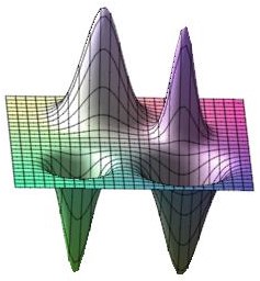 Figure 1
Peer Reviews
No public reviews on file for this paper yet. If you reviewed it on a platform where reviews are public (OpenReview, ICLR, NeurIPS, ICML), you can paste yours below so the community can read it here.
Videos
No videos yet. Explain this paper in a talk, walkthrough, or lecture? Add one.
Coexisting Vortices and Antivortices
Generated by Dually Gauged Harmonic Maps
Xiaosen Han
Institute of Contemporary Mathematics
School of Mathematics
Henan University
Kaifeng, Henan 475004, P. R. China
Genggeng Huang
School of Mathematical Sciences
Fudan University
Shanghai 200433, P. R. China
Yisong Yang
Courant Institute of Mathematical Sciences
New York University
New York, New York 10012, USA
Abstract
In this paper we first formulate a dually gauged harmonic map model, suggested from a product Abelian Higgs field theory arising in impurity-inspired field theories, and obtain a new BPS system of equations governing coexisting vortices and antivortices, which are topologically characterized by the first Chern class of the underlying Hermitian bundle and the Thom class of the associated dual bundle. We then establish existence and uniqueness theorems for such vortices. For the equations over a compact surface, we obtain necessary and sufficient conditions for the existence of solutions. For the equations over the full plane, we obtain all finite-energy solutions. Besides, we also present precise expressions giving the values of various physical quantities of the solutions, including magnetic charges and energies, in terms of the total numbers of vortices and antivortices, of two species, and the coupling parameters involved.
Key words. Gauge field theory, harmonic maps, magnetic vortices, mixed states, impurities, topological invariants
PACS numbers. 02.30.Jr, 02.30.Xx, 11.15.-q, 74.25.Ha
MSC numbers. 35J50, 53C43, 81T13
1 Introduction
Vortices in quantum field theory were first conceptualized in the pioneering work of Abrikosov [1] in his prediction of the onset of type-II superconductivity characterized by the appearance of mixed states, due to the celebrated Meissner effect, in the context of the Ginzburg–Landau theory [17, 58]. In such a formalism electromagnetism is classically governed by a massive Maxwell equation, also known as the London equation [31, 58], but the order parameter is quantum-mechanically governed by a nonlinear gauged Schrödinger equation, giving rise to a quantum current density to sustain electromagnetism. Since then vortices have been realized and recognized broadly in applications and theoretical investigations in areas ranging over condensed-matter physics, elementary particle physics, and cosmology. Naturally, the richness of applications of vortices has prompted considerable extensions of the theory beyond the minimally coupled Ginzburg–Landau theory, which are characterized by the presence of multiple scalar and gauge fields introduced to fulfill various theoretical and phenomenological purposes. Notably, in the relativistically extended Ginzburg–Landau theory known as the Abelian Higgs theory, vortices appear as the Nielsen–Olesen strings [38] which serve to mediate in a type-II superconductor the interaction between a monopole and an anti-monopole resulting in a constant attractive force between the pair which would confine the monopoles [32, 33, 36, 56, 57]. This idea motivated Seiberg and Witten [46] to arrive at a similar mechanism aimed to resolve the quark confinement puzzle. In such an extended setting, numerous supersymmetric gauge field theory models are used and the classical Meissner effect is supersymmetrically expanded so that the Nielsen–Olesen magnetic strings, as well as magnetically charged monopoles, assume the forms of correspondingly revised, colored, counterparts [4, 12, 13, 15, 19, 22, 23, 35, 48, 49], to realize a linear confinement picture [14, 18, 29, 47, 50, 51, 59]. In these studies the full vortex, or the complete vortex-monopole complex [9, 53], equations are too difficult to analyze. Instead, people have relied on exploring the underlying, much reduced BPS structure (after the earlier works of Bogomol’nyi [7] and Prasad and Sommerfeld [41] on the Yang–Mills–Higgs monopoles and dyons) for the vortex equations. Besides, in [64], Witten considered a two-Higgs extended Abelian Higgs model which serves to generate cosmic strings as seeds for matter accretion for the galaxy formation in the early universe [27, 28, 61, 62]; in [5], Babaev studied a two-flavor Ginzburg–Landau theory aimed at modeling two-gap superconductivity which gives rise to fractionally magnetized vortices absent in conventional single-gap situations; in [10, 25], some two-Higgs particle extensions of the Abelian Higgs theory are used to describe double-layer fractional quantum Hall effect in terms of the Chern–Simons kinetics. These and other applications have led to some active research on vortices generated in quantum-field theory models accommodating extended gauge and matter field dynamics. Motivated by these studies, in the present work, we consider coexisting vortices and antivortices, carrying opposite magnetic charges, arising in a field theory containing two Higgs scalar fields generated from two gauged harmonic maps. This problem owes its origin from several subjects of distinguished interest and significance in field theories: Firstly, it originates from the classical integrable sigma model studied by Belavin and Polyakov [6] where the configuration map is the spin vector describing the magnetic orientation in a ferromagnet which is mathematically the simplest harmonic map of a nontrivial topological characterization [11]. Secondly, its gauge-theoretical content was initially explored by Schroers [44, 45] to host electromagnetism, whose elegant BPS structure enabled an Abelian Higgs theory [65, 66], in which vortices and antivortices of opposite magnetic charges coexist, to be developed. Thirdly, and more recently, electric and magnetic impurities are considered in the Abelian Higgs model in the context of supersymmetric field theories and the usual BPS structure is shown to be preserved in the presence of such impurities [24]. In particular, in [60], Tong and Wong proposed that magnetic impurities may be viewed as heavy, frozen vortices sitting in an additional Abelian gauge group, so that the interaction of the Abelian Higgs vortices with impurities may be described in the framework of a product Abelian gauge field theory with two scalar fields, which was later shown [21] to enjoy a general product Abelian gauge-field-theory formalism, allowing an extension to include the Chern–Simons dynamics as well. Inspired by these studies, we shall develop in the present work a product Abelian gauge field theory which accommodates four species of oppositely charged and multiply distributed BPS vortices induced from two Higgs fields. Specifically a solution would possess two species of positively charged vortices of the vortex numbers and two species of negatively charged vortices of the vortex numbers , respectively. We will present existence and uniqueness theorems for such vortex solutions under necessary and sufficient conditions given explicitly in terms of , and other physical parameters in our field-theoretical framework. The rich properties of these solution configurations may be useful in offering broader vortex phenomenologies in quantum field theories, in view of [5, 10, 14, 18, 25, 27, 28, 29, 47, 50, 51, 59, 61, 62, 64, 65, 66], for example, and elsewhere, and stimulate further exploration.
The rest of the paper is organized as follows. In the next section, we first review the bare [6, 42, 43] and gauged [44, 45, 52, 65, 66] harmonic models for the purpose of illustrating how vortices of opposite vortex charges arise and what new properties are to be expected. We then present a dually gauged harmonic map model hosting two interacting harmonic maps and gauge fields along the line of a product Abelian Higgs theory accommodating impurities [24, 60]. We will derive a new BPS system of equations and demonstrate how two species of vortices and antivortices arise. We will also show how this system of equations reduces into the system that arises in the product Abelian Higgs theory [20] recently uncovered to extend the formalism in [60]. In Section 3, we state our existence and uniqueness theorems for solutions of the BPS systems of equations over a compact surface and on the full plane. Our mathematical analysis is based on calculus of variations and elliptic a priori estimates. Specifically, in Section 4, we prove the theorem in the compact-surface situation. Technically, the governing functional assumes a logarithmic form which makes the underlying analytic structure more difficult from those already investigated in the literature. In our situation, fortunately, we encounter two logarithmic terms which may be seen to compensate each other in such a way that, jointly, they give rise to a linear lower bound, thus enabling a resolution to the logarithmic difficulty. In Section 5, we establish the theorem in the full-plane situation. In this situation, it is difficult to get the coerciveness of the associated functional straightforwardly in the usual Sobolev space , due to the logarithmic nonlinear terms again, coupled with the issue associated with loss of compactness. To overcome this difficulty, we use some estimates which involve a combination of the -norm and the -norm of the minimizing sequence in two different domains, so as to achieve a desired energy control of the sequence. In our approach, we show how the difficulty may be resolved by our domain splitting method and the use of a special form of the Gagliardo–Nirenberg interpolation inequality so that a minimizing sequence is eventually shown to be bounded in . Thus a minimizer may be obtained as a weak limit of the sequence. These technical novelties lead us to a complete understanding of the problem of existence and uniqueness of solutions realizing two species of prescribed vortices and antivortices in the proposed dually coupled harmonic map model. In Section 6, we derive sharp exponential decay estimates and quantized integrals for a planar solution. In Section 7, we briefly summarize our work and make some comments.
2 Vortex equations induced from gauged harmonic maps
In this section, we aim to derive a dually gauged harmonic map field theory which allows the coexistence of vortices and antivortices. In order to motivate the derivation, we begin by a discussion of the gauged harmonic map model, especially its origins from the classical harmonic map model. We then derive the dually gauged theory and show how vortices and antivortices arise. We end the section to comment on a natural link of the solutions to harmonic maps.
2.1 Classical and gauged harmonic map models
Recall that in the classical (static) sigma model describing a planar ferromagnet the field configuration is a spin vector which maps into the unit sphere, , in , namely, . The energy then reads [6, 42, 43]
[TABLE]
Due to the finite-energy requirement, we may assume approaches a fixed vector at infinity. Thus, for , we may compactify so that belongs to a second homotopy class on characterized by its corresponding Brouwer degree, , which may be represented by the following normalized area integral,
[TABLE]
In view of (2.2), it is seen [6, 42, 43] that there holds the topological energy bound
[TABLE]
and that, in each class, solutions saturating the energy lower bound (2.3) could be constructed explicitly via meromorphic functions [6, 42]. On the other hand, in the gauged sigma model proposed in the work of Schroers [44], the energy (2.1) is extended to take the form
[TABLE]
where () is a vector field, the induced magnetic curvature, are covariant derivatives, and is the north pole on , and the degree formula (2.2) may be modified to assume the form
[TABLE]
so that the same energy bound (2.3) may be established. Here we emphasize that this construction relies on the structure of the energy (2.4) which specifies a fixed groundstate, , at the infinity of , enabling its compactification into as before, thus the validity of the degree formula (2.5). Of course this form of the energy breaks the original symmetry in the bare energy (2.1). To exploit the broken symmetry and explore the electromagnetism induced from the gauge field, in [45], Schroers revisited the gauged sigma model and formulated the theory into a general setting, whose energy essentially assumes the form
[TABLE]
where determines the angle between the north pole and at infinity in . In particular, when , the set of groundstates, or vacua, becomes a circle manifold defined by the equations
[TABLE]
so that the theory possesses a spontaneously broken symmetry which leads to the appearance of vortices and antivortices, as in the Ginzburg–Landau theory [1, 17]. As a consequence, a new Abelian Higgs theory naturally arises. In fact, without loss of generality, take and consider a complex scalar field induced from the map so that
[TABLE]
That is, we project onto the complex plane through the south pole , which corresponds to infinity of . Thus, with the induced gauge-covariant derivatives (), the normalized energy density given in (2.6) becomes
[TABLE]
There are two interesting and relevant facts worthy noticing.
(i) Like that in the classical Yang–Mills–Higgs theory, the potential density function for the complex scalar field also has a Mexican-hat profile. In particular, when we take the limit in the denominators of the second and third terms in (2.9), we see that the model approaches that of the classical Abelian Higgs theory,
[TABLE]
for which an existence and uniqueness theorem for multiply distributed vortices was established over in [26, 54, 55] and over a compact surface in [8, 39, 40, 63] where it is shown that the total vortex number needs to satisfy the bound
[TABLE]
in which being the surface area of , to ensure existence of a BPS solution. The bound given in (2.11) is sometimes referred to as the Bradlow bound [2, 34, 37].
(ii) The preimages of the north pole under the original spin vector become the zeros of the complex field and those of the south pole the poles of . Moreover, the energy density (2.9) is invariant under the transformation
[TABLE]
in addition to its gauge invariance. This important feature indicates that the poles and zeros will play equal roles. Specifically, the magnetic field may be shown to be governed in the BPS limit of the equations of motion of (2.9) by the formula [44, 65, 66]:
[TABLE]
so that the zeros and poles of give rise to vortices with and antivortices with , respectively, and that the total energy reads
[TABLE]
where are the numbers (counting algebraic multiplicities) of zeros and poles of , which are also the total vortex and antivortex numbers of the system. Furthermore, the Bradlow bound (2.11) is now replaced with the updated bound [52]
[TABLE]
which implies that the total vortex number, , and thus the energy as well, as given in (2.14), may be arbitrarily high, so far as the discrepancy of the two types of the vortices, measured by the quantity , remains under control by (2.15).
2.2 Dually gauged harmonic map model with two interacting configuration maps
We are now prepared to consider a dually gauged harmonic map (or sigma) model, with two interacting configuration maps, , with images in , and two Abelian gauge fields, , in the static situation (for simplicity). As before, use and to denote the magnetic fields induced from and , respectively. Let
[TABLE]
be the covariant derivatives associated with the charge parameters . It can be seen that there holds the identity
[TABLE]
where (the same for ) with
[TABLE]
A similar expression for also holds. Hence we have the degree formula
[TABLE]
provided that at infinity of . A similar expression holds for . Hence, combining these facts with the methods in [7, 41, 44], we arrive at the BPS energy density
[TABLE]
which leads to the following extended potential density function in view of (2.6):
[TABLE]
where are coupling parameters. Thus, corresponding to the symmetric vacuum state case,
[TABLE]
at infinity, we have , and to the spontaneously broken symmetry case,
[TABLE]
at infinity, we have
[TABLE]
similar to the case in (2.6). Therefore, in this latter case, we can write down the normalized energy density governing the scalar fields coupled with the gauge fields as
[TABLE]
In order to illustrate the topological structure of the model more transparently, we now represent the maps by a pair of complex scalar fields , via formulas like (2.8) leading to the relation
[TABLE]
between and , and similarly for and , realized as two cross sections over a Hermitian line bundle over a Riemann surface , either compact or non-compact, and the gauge fields as two connection 1-forms which induce the magnetic fields as curvature 2-forms , with the connections
[TABLE]
operating on , respectively, where are seen to be real coupling parameters, whose roles are to mix the interaction of . Thus, with this notation, the energy density (2.25) becomes
[TABLE]
where is the Hodge dual. So it follows that the Euler–Lagrange equations of (2.28) are
[TABLE]
which are rather complicated. It is interesting to note that, in the limit , (2.28) becomes
[TABLE]
which has been studied in [21] so that the Abelian Higgs theory with impurity studied in [60] corresponds to the choice . For (2.33), the Euler–Lagrange equations, or the generalized two-gap Ginzburg–Landau equations in our context, are
[TABLE]
Setting in the denominators in (2.28), (LABEL:2.19)–(2.32), we can recover (2.33), (2.34)–(2.37), respectively.
We now pursue a BPS reduction to the full governing equations (LABEL:2.19)–(2.32). To this goal, recall the identities
[TABLE]
[TABLE]
etc. Besides, for the current densities
[TABLE]
we have
[TABLE]
Hence, we obtain the energy decomposition
[TABLE]
Applying (2.42), (2.43) in (2.44), we arrive at the neat expression
[TABLE]
Observe that the quantities
[TABLE]
are related to the first Chern classes represented by the curvature 2-forms , respectively, and
[TABLE]
the Thom classes of the dual bundle of , represented by the mixed gauge connections , respectively. For some detailed computation and characterization of these topological invariants, see [52]. Thus
[TABLE]
is a topological density which yields via (2.45) the topological lower bound
[TABLE]
which is attained when satisfies the BPS equations
[TABLE]
Here and in the sequel we observe the convention that we choose either the upper or lower sign in all equations simultaneously. It is straightforward to examine that (2.50)–(2.53) imply (LABEL:2.19)–(2.32). Therefore, we have arrived at a significant reduction of the complicated system of equations (LABEL:2.19)–(2.32) into the system of equations (2.50)–(2.53), along the spirit of Bogomol’nyi [7] and Prasad–Sommerfield [41], which will be the focus of our study to follow.
We next explain how vortices and antivortices arise in the system of the BPS equations (2.50)–(2.53). First, the equations (2.50)–(2.51) indicate that are meromorphic so that their zeros and poles are isolated and of integer multiplicities. Thus, counting multiplicities, we may let the sets of zeros and poles of be denoted by
[TABLE]
respectively. That is, algebraically, have zeros and poles, respectively, as indicated. Then introduce
[TABLE]
as two induced magnetic fields. Consequently, in view of (2.52)–(2.53), we obtain
[TABLE]
so that vortices and antivortices are exhibited and presented by the zeros and poles of clearly, where attain their global maximum and minimum, , depending on the choice of signs, respectively.
Later, we will obtain the quantities
[TABLE]
which give rise to the associated first Chern classes
[TABLE]
where and are the curvature 2-forms induced from the connection 1-forms
[TABLE]
which take account of the the differences of the numbers of zeros and poles, of the sections , respectively, and solely. As another consequence, we are led to the following quantized values of the magnetic charges or fluxes
[TABLE]
which depend on the full spectrum of the numbers of the zeros and poles of both and .
As an illustration, in Figure 2.1, we present a plot of the strength of one of the two identified magnetic fields which peaks and valleys at the centers of one of the two species of vortices and antivortices represented by the zeros and poles of one of the two Higgs scalar fields descending from two coupled and gauged harmonic maps, respectively.
2.3 Notes on the analytic properties of solutions
Here we comment briefly on the analytic properties of the solution maps so constructed.
First, recall that the energy (2.1) is Dirichlet such that, when the range of is the full space rather than , a critical point of the energy is harmonic, . However, since the range of is confined to , a critical point of (2.1) satisfies, instead, the nonlinear equation
[TABLE]
whose solutions are much more complicated. (Although the “true harmonic” equation automatically implies (2.66), the finite-energy condition indicates that all solutions to are trivial, i.e., constant.) Nevertheless, the work of Belavin and Polyakov [6] establishes the fact that solutions of (2.66) are all given through the stereographic projection (2.8) by the solutions of the equation
[TABLE]
In other words, solutions of (2.66), away from isolated poles, are all represented by holomorphic or anti-holomorphic functions. Thus, the term “harmonic” is well justified.
Next, in the gauged harmonic map model governed by the energy (2.9) discussed in §2.1, the BPS equations consist of the vortex equation (2.13) and a “holomorphic equation” which reads [44, 45]
[TABLE]
thereby replacing the conventional derivatives in (2.67) by gauge-covariant derivatives. The equation (2.68) implies that, away from isolated poles, is indeed holomorphic or anti-holomorphic up to a smooth multiple [26]. In other words, we arrive at a similar “harmonic representation” of the field configurations through the “gauged holomorphic equation” (2.68).
Finally, in the context of the dually gauged theory studied in §2.2, the single gauged holomorphic equation (2.68) is now replaced by a pair of gauged holomorphic equations, (2.50) and (2.51), which govern , a pair of gauged holomorphic or anti-holomorphic sections.
Thus we have seen that in gauged models the configuration maps all lie in the category of harmonic maps with well-exhibited analytic features.
In the subsequent sections, we will construct solutions of the gauged harmonic map [44, 45, 52, 65, 66] and impurity [60], as well as [20], inspired BPS equations (2.50)–(2.53) realizing a prescribed distribution of vortices and antivortices, represented as zeros and poles of in (2.54) and (2.55), respectively.
3 Existence and uniqueness theorems for coexisting vortices and antivortices
In this section, we state our existence and uniqueness theorems for vortices and antivortices over a compact surface and on . We then present the system of nonlinear elliptic partial differential equations descending from the BPS equations (2.50)–(2.53) which govern such vortices and antivortices.
We first consider the equations over a compact Riemann surface equipped with a Riemannian metric and use to denote the associated canonical surface element.
Theorem 3.1**.**
Consider the BPS equations (2.50)–(2.53) of the energy density (2.28) formulated over a complex Hermitian line bundle over a compact Riemann surface with canonical total area governing two connection 1-forms and two cross sections . For the prescribed sets of zeros and poles for the fields and given respectively in (2.54) and (2.55), these coupled equations admit a solution with these sets of zeros and poles, if and only if
[TABLE]
Moreover, modulo gauge transformations, such a solution is unique and carries quantized magnetic charges (2.64) and (2.65), and minimum energy of the form
[TABLE]
which is seen to be stratified topologically by the Chern and Thom classes of the line bundle and its dual respectively. In particular, in terms of energy, zeros (vortices) and poles (antivortices) of and contribute equally.
We next consider the equations (2.50)–(2.53) over . We have the following theorem.
Theorem 3.2**.**
For the BPS equations (2.50)–(2.53) in and over with the prescribed sets of zeros and poles for the fields and given respectively in (2.54) and (2.55), modulo gauge transformations, there is a unique finite-energy solution realizing these sets of zeros and poles, which represent vortices and antivortices of opposite magnetic charges. Moreover, such a solution enjoys the sharp exponential decay estimates
[TABLE]
where is arbitrarily small and
[TABLE]
and carries quantized magnetic charges (2.64) and (2.65), now evaluated over , and minimum energy of the form
[TABLE]
given again in terms of the total numbers of vortices (zeros of ) and antivortices (poles of ) only.
The above two theorems will be obtained from Theorems 4.1 and 5.1, respectively, in the following two sections, except the energy formulas (3.2) and (3.5). In fact, as in [52], we may check that the Thom classes take the values
[TABLE]
similarly over , which with the help of the quantized integrals in Theorems 4.1 and 5.1 lead to the derivations of (3.2) and (3.5), respectively.
We now proceed to deduce the governing nonlinear elliptic partial differential equations of our problem. To this end, use to denote the Laplace–Beltrami operator on induced from the metric :
[TABLE]
Then, away from the zeros and poles of , we can resolve (2.50), (2.51) to obtain, the relations
[TABLE]
In view of these relations and (2.52)–(2.55), we see that satisfy the equations
[TABLE]
which govern two species of vortices and antivortices at the prescribed locations at and with and , , respectively.
Note again that, in the limit in the denominators of the nonlinearities and absence of poles, these equations reduce to those in [21] for the generalized Abelian Higgs equations, inspired by the work of Tong and Wong [60]. Such a property is elegant.
4 Vortices and antivortices on a compact surface
In this section we study the equations (2.50)–(2.53) over a compact Riemann surface , which have been reduced to the elliptic equations (3.11)–(3.10). To prove Theorem 3.1, we consider the following more general system of equations:
[TABLE]
where are constants satisfying , and
[TABLE]
Note that, for greater generality of our study, we will not assume symmetry for the coefficient matrix .
Let be solutions of
[TABLE]
with (cf. [3]). Set , , in (4.1)–(4.2). Then solves
[TABLE]
Consider the following functional over :
[TABLE]
In this section we use the following notation
[TABLE]
Then it is clear that (4.6) and (4.7) are the Euler–Lagrange equations of functional (4.8).
Theorem 4.1**.**
Suppose and . Then the system of equations (4.6)–(4.7) admits a solution if and only if
[TABLE]
Moreover, if the solution exists, it is unique and there hold the following quantized integrals
[TABLE]
Proof.
We first prove that (4.10) is a necessary condition. If there is a solution of (4.6)–(4.7), then after a direct computation we have
[TABLE]
Then the quantized integrals (4.11)–(4.12) follow from a direct integration of (4.13)–(4.14) over . Noting the elementary inequality for any , we can get the necessity of (4.10) from (4.11)–(4.12).
We now turn to the proof of sufficiency of (4.10). Notice the elementary inequality
[TABLE]
which implies
[TABLE]
Then by (4.10) and (4.16), there exists positive constants such that
[TABLE]
which says that the functional is bounded from below. Using (4.17) and Poincaré inequality, we observe also that the functional is coercive in a well understood sense. Then the minimization problem
[TABLE]
is well posed.
Consider a minimizing sequence . Then we can easily see that, for some positive constant ,
[TABLE]
Set with . Then by the Moser–Trudinger inequality [3, 16]
[TABLE]
where is a constant, and the Poincaré inequality, we have
[TABLE]
From (4.17) we can see that . This implies is weakly compact in . Then, up to a subsequence, there exists such that weakly as . Consequently, is a minimizer of the functional , which gives a weak solution of the system (4.6)–(4.7). A standard bootstrap argument then shows that it is also a smooth solution.
For the uniqueness part, we just need to show the minimizer is unique. It is a consequence of the fact that the functional is strictly convex, which can be checked straightforwardly, thereby completing the proof. ∎
5 Planar solution: proof of existence by minimization
To prove Theorem 3.2, we consider (4.1)–(4.2) over subject to the boundary condition
[TABLE]
We have the following main existence and uniqueness theorem.
Theorem 5.1**.**
Suppose and . Then the system of equations (4.1)–(4.2) over admits a unique solution satisfying (5.1). Moreover, the solution enjoys the following sharp decay estimates
[TABLE]
for being sufficiently large, where is arbitrarily small, a corresponding constant, and given by the formula
[TABLE]
Furthermore, there hold the quantized integrals
[TABLE]
We now proceed to prove the existence and uniqueness of a solution by the method of calculus of variations. The stated decay estimates and quantized integrals of a solution will be established in the next section.
Let be given by
[TABLE]
By a direct computation, we have
[TABLE]
where
[TABLE]
Note that
[TABLE]
which implies as uniformly for . Fix large to be determined later. Also from the above construction, we know , .
Set , . Then we reduce (4.1)–(4.2) and (5.1) into
[TABLE]
over and
[TABLE]
respectively.
We now consider the functional for as follows:
[TABLE]
where and in the sequel we use the notation
[TABLE]
Now we show that the functional is well defined. We split into two parts:
[TABLE]
Then we have
[TABLE]
On the other hand, from , we obtain in . Thus, we have
[TABLE]
The bounds (5.17)–(5.18) establish that the functional is well defined. In fact, in line of these estimates, it becomes clear to show that is over . Thus, as in the compact case, it is seen that the equations (5.11)–(5.12) are the Euler–Lagrange equations of the functional given in (5.14). Note also that the functional is strictly convex. So has at most one critical point in . In particular the uniqueness of a solution of (5.11)–(5.12) in follows.
Next, we aim to get some lower control of the functional. For convenience, we modify the splitting (5.16) slightly:
[TABLE]
On , using Taylor’s truncation, we have
[TABLE]
On the other hand, on , we have
[TABLE]
Then we see that
[TABLE]
where are some positive constants.
Furthermore, for the last two terms in (5.14), we have
[TABLE]
where is a constant to be determined later.
Combining (5.20), (5.22), and (5.23), and noting the fact that for any and as uniformly for , and that in (5.23) may be chosen to be small, we arrive at
[TABLE]
where are positive constants independent of . In particular, we see that the functional is bounded from below in the space such that the minimization problem
[TABLE]
is well-defined, as in the compact surface situation.
Consider a minimizing sequence . We need to show is a bounded sequence in . In what follows we use to denote and to denote the corresponding () defined in (5.24) associated with the pair . From (5.24), we have the bound
[TABLE]
for some constant . Now, for any fixed , we have
[TABLE]
and
[TABLE]
Now consider the open set . Without loss of generality, we assume . Let
[TABLE]
By (5.27), we know . Also since is compactly supported, is a bounded open set. Define
[TABLE]
Then, from the above analysis, we have
[TABLE]
Recall a special case of the Gagliardo–Nirenberg interpolation inequality (cf. Theorem 12.83 in [30]):
[TABLE]
Taking in (5.32) and applying it to , we see that, in view of (5.31), there holds the bound
[TABLE]
where is a constant independent of . This in turn implies
[TABLE]
where is a constant independent of .
Likewise, for (say), there also holds
[TABLE]
with an -independent positive constant .
From the estimates (5.28), (5.34), and (5.35), we see that the sequence is bounded in . That is, the minimizing sequence is bounded in .
Then, taking a subsequence if necessary, we may assume that weakly in , and a.e. in for some , . Noting that the functional is in and weakly lower semicontinuous, which is ensured by its convexity, we see that . As a (unique) critical point of in , is a weak solution of (5.11)–(5.12).
We may check that the right-hand sides of the system of equations (5.11)–(5.12) belong to . Then by the standard elliptic -estimates we have , which implies as , . Furthermore, a bootstrap argument shows that is a smooth solution of (5.11)–(5.12).
6 Planar solution: exponential decay properties and quantized integrals
Now we first establish the decay estimates of the planar solution at infinity.
Let satisfy
[TABLE]
and denote a disk in centered at the origin with radius . Then, outside , we may conveniently rewrite (4.1)–(4.2) as
[TABLE]
where
[TABLE]
is a positive definite matrix whose smaller eigenvalue is
[TABLE]
Let . Noting that vanish at infinity, after a direct computation, we have
[TABLE]
where is a function vanishing at infinity. Then, for any , there exists an such that
[TABLE]
where
[TABLE]
Hence by (6.6) and a comparison function argument we infer that, for any , there exists a constant such that
[TABLE]
Next, let denote any of the two derivatives, and . Thus, when , we have
[TABLE]
Noting that the right-hand side of (6.9) belongs to and using the elliptic -estimate there, we obtain , which implies in particular that and vanish at infinity.
Rewrite (6.9) again as before in the familiar form:
[TABLE]
where is given in (6.3). Set . Then we have
[TABLE]
where is a function vanishing at infinity. Thus, similar as in getting (6.8), we deduce that, for any , there exists a constant such that
[TABLE]
where is defined as in (6.7). Therefore, the desired estimates (5.2)–(5.3) follows from (6.8) and (6.12).
Finally we derive the quantized integrals. To proceed, we note that, in view of the properties of stated in (5.3) and of given in (5.7) (), we have (say) as , . As a consequence, the divergence theorem then leads to
[TABLE]
Besides, a direct integration gives us
[TABLE]
Combining (6.13) and (6.14), we obtain
[TABLE]
from which the anticipated quantized integrals (5.5)–(5.6) then follow.
7 Summary and comments
Extended quantum field theory models hosting multiple sectors of the Higgs fields are of wide range of applications including superconductivity, elementary particles, condensed-matter physics, and cosmology. In these applications, vortices, or vortexlines, often provide useful conceptual constructs and mechanisms for interactions at fundamental levels. Thus, realization and uncovery of vortices of novel features are of value. In this work, we developed a gauge field theory allowing the coexistence of vortices and antivortices and established a series of sharp existence and uniqueness theorems for the solutions of the governing equations.
- (i)
Based on the gauged harmonic map model and the product Abelian Higgs theory hosting impurities, an extended and dually coupled gauged harmonic map model is presented in which two species of vortices and antivortices coexist and are governed by vortex equations of a BPS type. Topologically, the solutions are characterized by two classification classes, namely, the first Chern class of the defining line bundle and the Thom class of the associated dual bundle. Mathematically, the vortices and antivortices of solutions are given by the zeros and poles of the cross-sections where two induced magnetic fields represented by bundle curvatures attain their peaks and valleys. 2. (ii)
For the vortex equations over a compact surface modeling a doubly periodic lattice structure, an existence and uniqueness theorem for a solution realizing an arbitrarily given prescribed distribution of vortices and antivortices is proved under a necessary and sufficient condition relating the total numbers of vortices and antivortices and the coupling parameters involved. This condition is independent of the locations of the vortices but gives an explicit upper bound for the differences of the numbers of vortices and antivortices in terms of the total area of the hosting surface. 3. (iii)
For the vortex equations over the full plane, an existence and uniqueness theorem for coexisting vortex and antivortex solutions is also proved for arbitrary coupling parameters and vortex numbers. The solutions describe spontaneously broken vacuum symmetry at spatial infinity and are energetically localized configurations. Sharp exponential decay estimates of the solutions are obtained as well. 4. (iv)
The magnetic fluxes and energies of the solutions over a compact surface and on the full plane are all quantized and expressed in the terms of total numbers of vortices and antivortices. Specifically, the magnetic fluxes are determined by the differences of numbers of vortices and antivortices, suggesting the fact that magnetically these vortices annihilate each other, and the energy on the other hand is given in terms of the sum of the total numbers of all vortices, indicating the fact that energetically these vortices make equal or indistinguishable contributions as field solitons.
This work opens some future directions to be explored further. For example, it will be interesting to investigate the solutions realizing an unbroken vacuum symmetry at infinity characterized by the boundary condition in (2.20) or in a slightly modified version of the system of equations (2.50)–(2.53) at infinity. It will also be interesting to study the problem of coexisting cosmic strings and antistrings when the model is coupled with the Einstein gravity, especially the issue how these vortices give rise to localized curvature distribution and how they determine the deficit angle and geodesic completeness of the induced gravitational metric at infinity.
In a broader context, this work belongs to the study of coexisting field-theoretical solitons carrying opposite soliton charges, among which one of the most interesting applications is to use a monopole and antimonopole pair to model a quark and antiquark pair in interaction, to probe the linear confinement mechanism of quarks, as briefly reviewed in Introduction. However, at the governing equation levels, there has been no successful construction of solutions realizing a monopole and antimonopole pair, in three-spatial dimensional settings. Our work here, on the other hand, is a construction of vortices and antivortices, either paired or unpaired, realizing opposite magnetic charges, in both compact and noncompact situations, in two-spatial dimensional settings. Hopefully, this lower-dimensional construction will offer useful insight for the investigation in higher-dimensional settings.
Acknowledgments. Han was supported by National Natural Science Foundation of China under Grant 11671120 and HASTIT (18HASTIT028). Huang was supported by National Natural Science Foundation of China under Grant 11871160. Yang was partially supported by National Natural Science Foundation of China under Grant 11471100.
The reference list from the paper itself. Each links out to its DOI / PubMed record.
- 1[1] A. A. Abrikosov, On the magnetic properties of superconductors of the second group, Sov. Phys. JETP 5 (1957) 1174–1182.
- 2[2] C. Adam, J. M. Speight, and A. Wereszczynski, Volume of a vortex and the Bradlow bound, Phys. Rev. D 95 (2017) 116007.
- 3[3] T. Aubin, Nonlinear Analysis on Manifolds: Monge–Ampere Equations , Springer, Berlin and New York, 1982.
- 4[4] R. Auzzi, S. Bolognesi, J. Evslin, K. Konishi, and A. Yung, Nonabelian superconductors: vortices and confinement in 𝒩 = 2 𝒩 2 {\cal N}=2 SQCD, Nucl. Phys. B 673 (2003) 187–216.
- 5[5] E. Babaev, Vortices with fractional flux in two-gap superconductors and in extended Faddeev model, Phys. Rev. Lett. 89 (2002) 067001.
- 6[6] A. A. Belavin and A. M. Polyakov, Metastable states of two-dimensional isotropic ferromagnets, JETP Lett. 22 (1975) 245–247.
- 7[7] E. B. Bogomol’nyi, The stability of classical solutions, Sov. J. Nucl. Phys. 24 (1976) 449–454.
- 8[8] S. Bradlow, Vortices in holomorphic line bundles over closed Kähler manifolds, Commun. Math. Phys. 135 (1990) 1–17.