On Nitsche's method for elastic contact problems
Tom Gustafsson, Rolf Stenberg, Juha Videman

TL;DR
This paper analyzes Nitsche's method for elastic contact problems, establishing quasi-optimality and error estimates, and demonstrating its robustness and efficiency through numerical experiments.
Contribution
It introduces three Nitsche's mortaring techniques for contact boundary stabilization with minimal regularity requirements and no saturation assumption.
Findings
Nitsche's method is robust for elastic contact problems.
A posteriori error estimators are effective.
Numerical experiments confirm theoretical results.
Abstract
We show quasi-optimality and a posteriori error estimates for the frictionless contact problem between two elastic bodies with a zero-gap function. The analysis is based on interpreting Nitsche's method as a stabilised finite element method for which the error estimates can be obtained with minimal regularity assumptions and without the saturation assumption. We present three different Nitsche's mortaring techniques for the contact boundary each corresponding to a different stabilising term. Our numerical experiments show the robustness of Nitsche's method and corroborates the efficiency of the a posteriori error estimators.
Click any figure to enlarge with its caption.
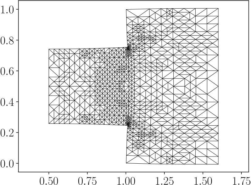 Figure 1
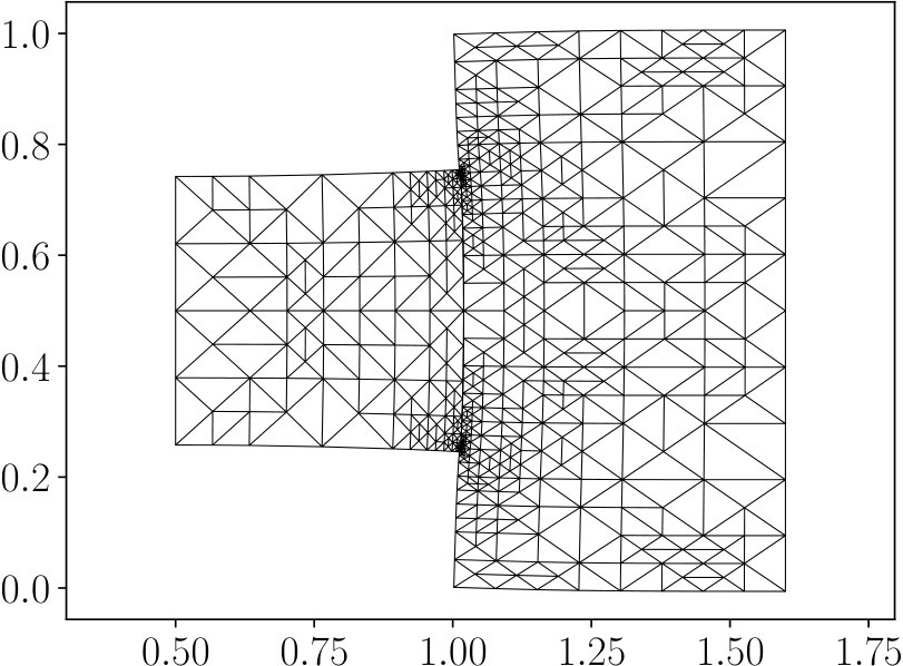 Figure 2
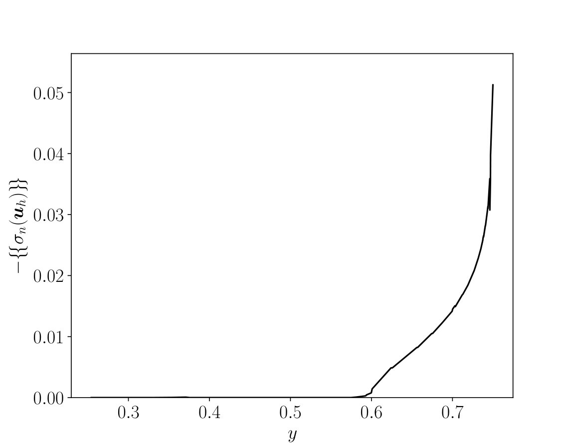 Figure 3
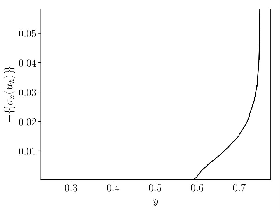 Figure 4
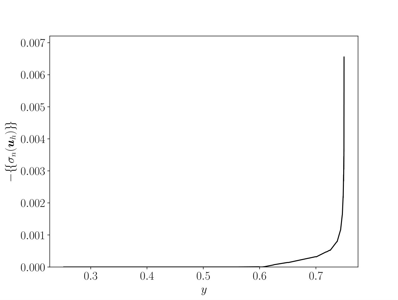 Figure 5
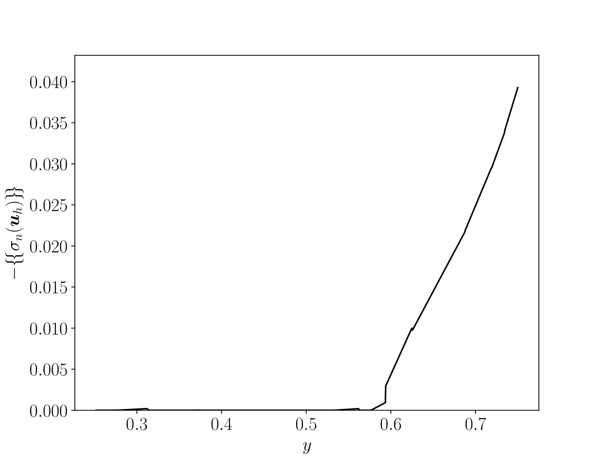 Figure 6
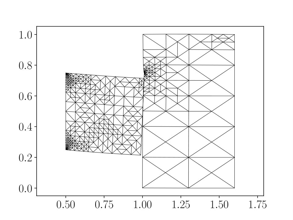 Figure 7
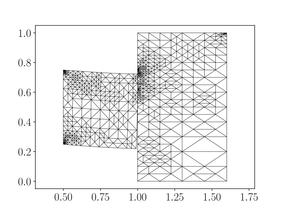 Figure 8
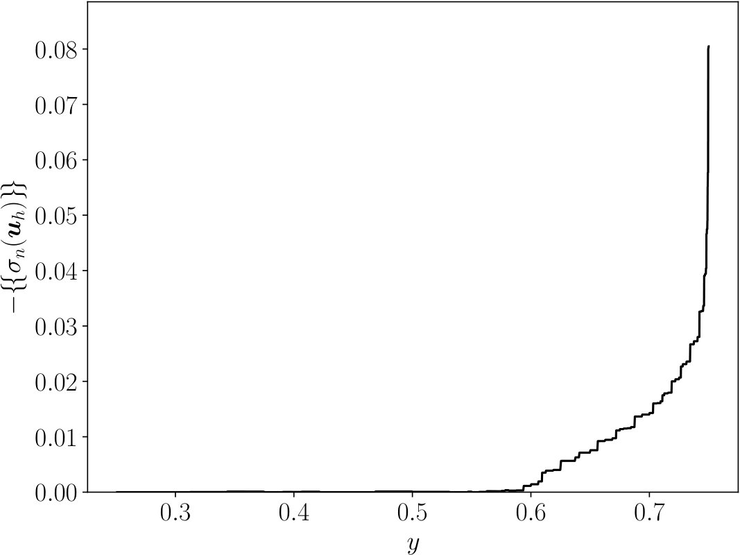 Figure 9
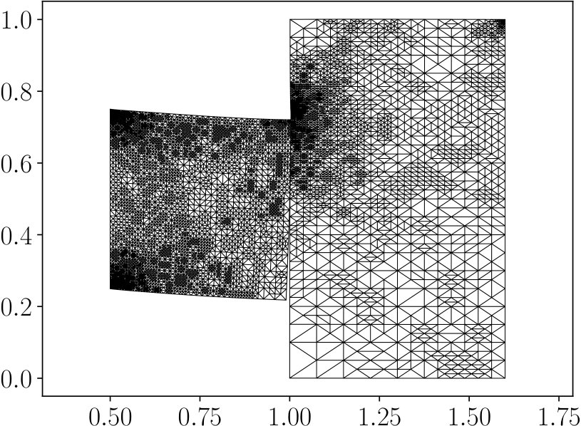 Figure 10
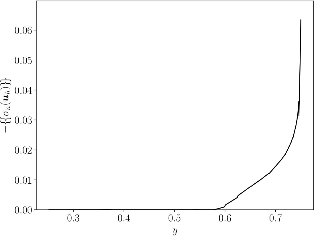 Figure 11
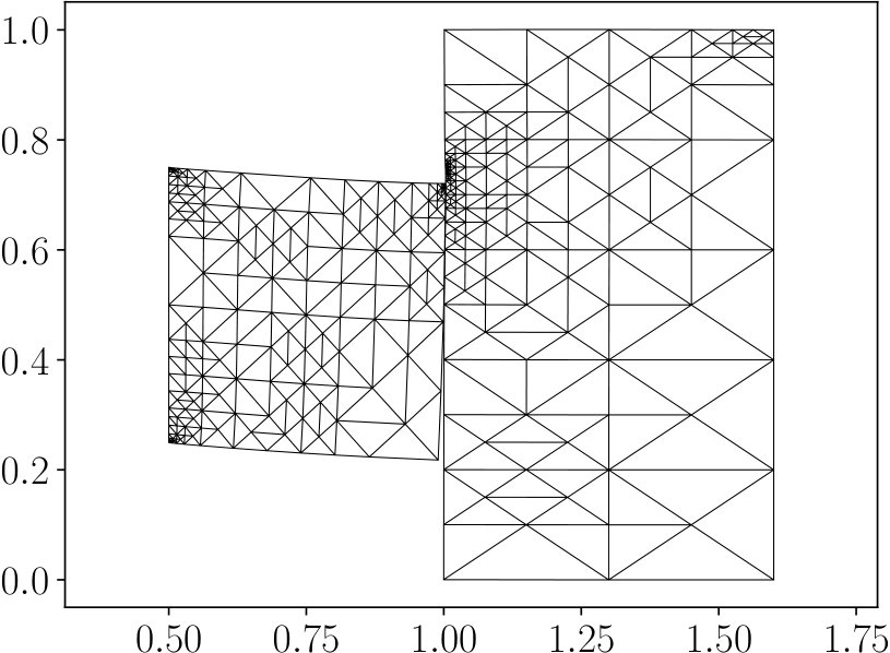 Figure 12
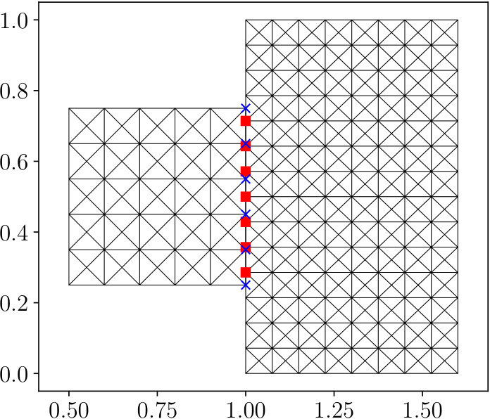 Figure 13
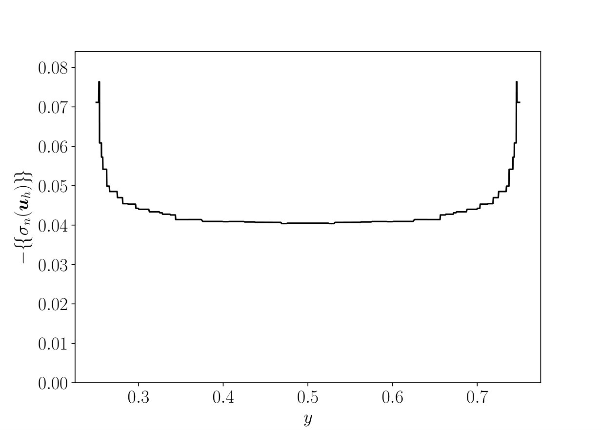 Figure 14
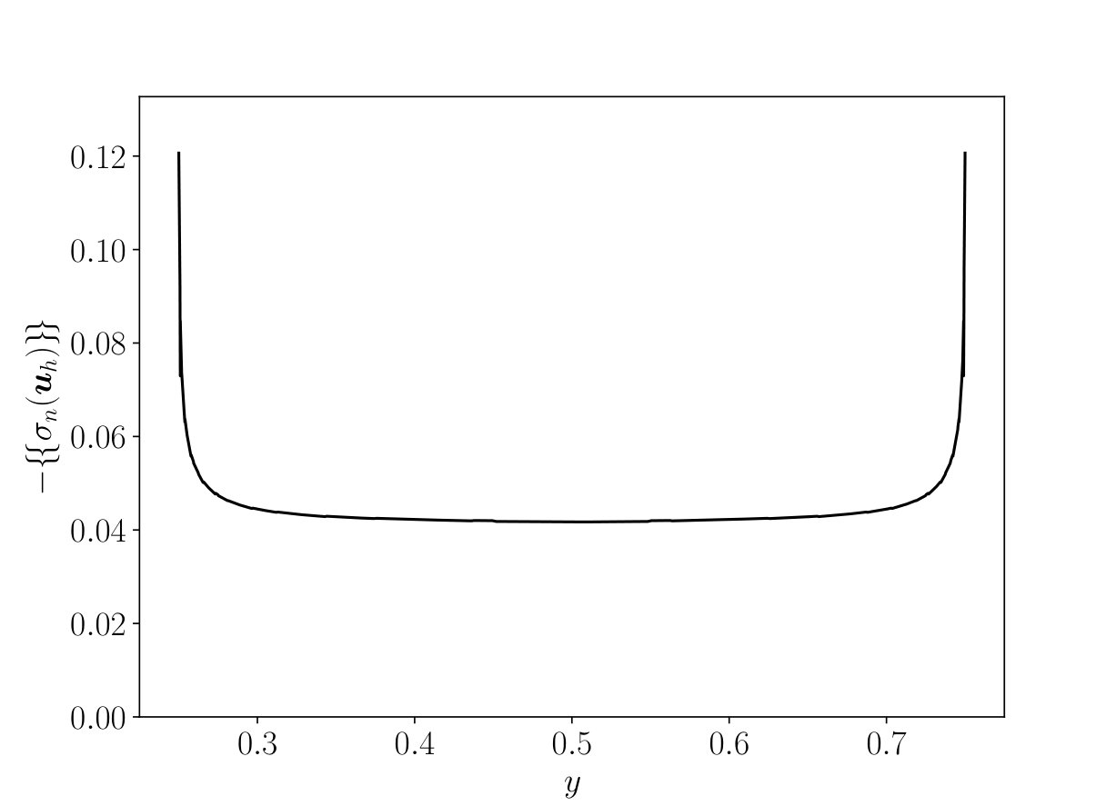 Figure 15
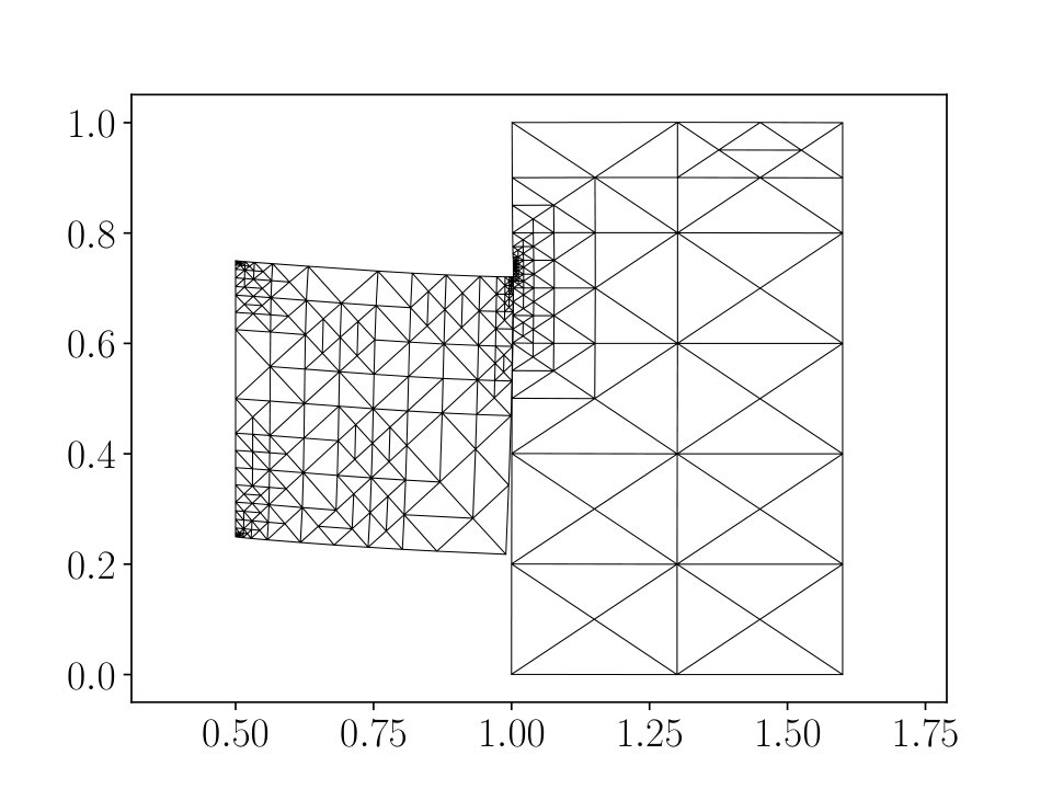 Figure 16
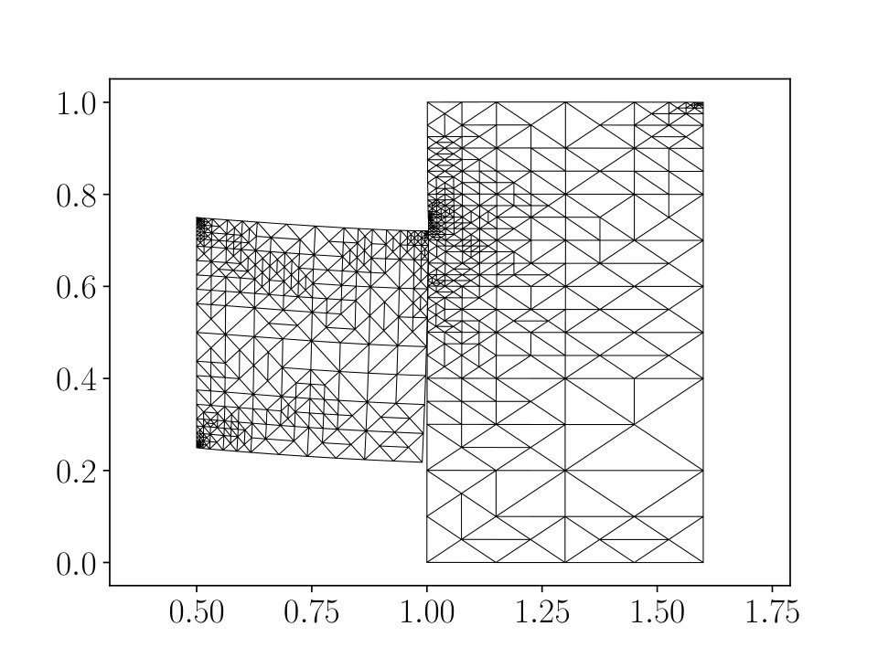 Figure 17
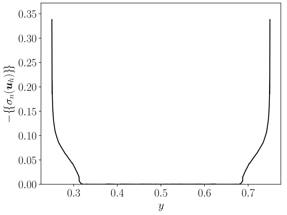 Figure 18
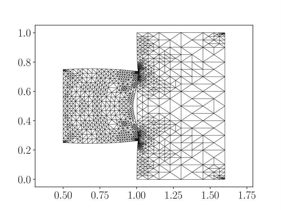 Figure 19
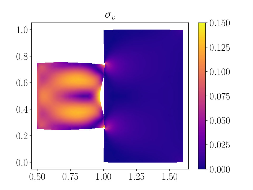 Figure 20
Peer Reviews
No public reviews on file for this paper yet. If you reviewed it on a platform where reviews are public (OpenReview, ICLR, NeurIPS, ICML), you can paste yours below so the community can read it here.
Videos
No videos yet. Explain this paper in a talk, walkthrough, or lecture? Add one.
On Nitsche’s method for elastic contact problems
Tom Gustafsson
Department of Mathematics and Systems Analysis, Aalto University, 00076 Aalto, Finland
,
Rolf Stenberg
Department of Mathematics and Systems Analysis, Aalto University, 00076 Aalto, Finland
and
Juha Videman
CAMGSD/Departamento de Matemática, Universidade de Lisboa, Universidade de Lisboa, 1049-001 Lisbon, Portugal
Abstract.
We show quasi-optimality and a posteriori error estimates for the frictionless contact problem between two elastic bodies with a zero-gap function. The analysis is based on interpreting Nitsche’s method as a stabilised finite element method for which the error estimates can be obtained with minimal regularity assumptions and without the saturation assumption. We present three different Nitsche’s mortaring techniques for the contact boundary each corresponding to a different stabilising term. Our numerical experiments show the robustness of Nitsche’s method and corroborates the efficiency of the a posteriori error estimators.
The financial support from the Portuguese government through FCT (Fundação para a Ciência e a Tecnologia), I.P., under the projects PTDC/MAT-PUR/28686/2017 and UTAP-EXPL/MAT/0017/2017, is gratefully acknowledged.
1. introduction
In this paper, we analyse the Nitsche method for elastic contact problems. Over the last decade, this method has been studied by a number of authors, see, e.g., [9, 6, 7, 10], and shown to be a robust and efficient method. The advantages are an easy implementation based on the displacement variables only and, when compared to mixed methods with Lagrange multipliers, the absence of an ”inf-sup” stability condition which renders a symmetric positive definite system instead of one with a saddle point structure.
From a theoretical point of view, the previously mentioned works suffer from two shortcomings. First, for the problem posed in , the solution is typically assumed to be in , with . Second, the a posteriori error analyses are often based on a non-rigorous saturation assumption.
We have addressed these issues in our recent articles, cf. [12, 13]. Our approach dates back to [23] where different ways to enforce weakly the Dirichlet boundary conditions were discussed in the context of the so called stabilised mixed methods [2, 3] wherein the bilinear form of the original mixed finite element method is augmented with a properly weighted residual term to ensure stability. In [23], it was shown that the local elimination of the Lagrange multiplier leads essentially to a method introduced by Nitsche in the early age of the finite element analysis [22]. Since Nitsche’s method is straightforward both to analyse (under the additional smoothness assumption) and to implement, we started to advocate it, in particular for contact problems, cf. [24, 4].
What we have realised recently is that one should take full advantage of the relation between Nitsche’s and stabilised method when analysing the former. In fact, we were able to get rid of both the smoothness and the saturation assumption for the membrane obstacle problem in [12]. In this paper, we will continue on this path and perform an error analysis, both quasi-optimality and a posteriori, for a simplified two-body contact problem without friction. Besides the theoretical improvements, we present three versions of the Nitsche’s method where the changes in the material parameters between the bodies are taken into account. The simplest is a typical ”master-slave” approach where the contact surface of the stiffer body is chosen as the master part and the slave surface is then mortared by the Nitsche’s technique. In the two other variants, the material parameters appear as weights in the Nitsche formulation so that the methods decide by themselves which part is the master and which is the slave. In order to simplify the notation, analysis and implementation of the adaptive methods, we assume that the elastic bodies are initially in full contact, see, e.g., [17], and leave the case with a non-vanishing initial gap between the elastic bodies for a future work.
Although our analysis is built upon our earlier works, cf. [12, 14], we will present proofs of all the main theorems. We also note that the elastic contact problem literature is vast and therefore we only refer to the review paper [27], and to all the references therein, for the analysis and application of finite element methods arising from mixed formulations and to [20, 8], and to all the references therein, for the a posteriori error analyses of contact problems. We end the paper by presenting results of our computational experiments.
2. The contact problem
Let , , , denote two elastic bodies in their reference configuration and assume that the bodies are initially in contact. Moreover, assume that are polygonal (polyhedral) domains and denote by their common boundary. The boundary is split into three disjoint sets and , with denoting the part where homogeneous Dirichlet data is given, the part with a Neumann boundary condition and the part where contact can occur, see Figure 1.
Letting , , be the displacement of the body , the infinitesimal strain tensor is defined as
[TABLE]
We assume homogenous isotropic bodies and a plain strain problem in the two dimensional case. The stress tensor is thus given by
[TABLE]
where is the shear modulus and the second Lamé parameter of the body and denotes the -dimensional identity tensor. We will exclude the possibility that the materials are nearly incompressible and hence it holds . (For nearly incompressible materials the standard approach of reformulating the problem in mixed form [5] should be used.)
By we denote the outward unit normal to , and define . In what follows, denotes any unit vector that satisfies .
We decompose the traction vector on , , into its normal and tangential parts, viz.
[TABLE]
For the scalar normal tractions we use the sign convention
[TABLE]
and
[TABLE]
and note that on these tractions are either both zero or continuous and compressive, i.e. it holds that
[TABLE]
The physical non-penetration constraint on reads as
[TABLE]
which, defining
[TABLE]
can be written as
[TABLE]
where \left\llbracket\cdot\right\rrbracket denotes the jump over .
We thus have the following problem.
Problem 1** (Strong formulation).**
Find , , , such that
[TABLE]
where denotes the volume force on .
Letting denote a Lagrange multiplier associated with the contact constraint, we obtain an equivalent mixed formulation in which the normal traction on the contact surface is an independent unknown.
Problem 2** (Mixed formulation).**
Find , , , and , such that
[TABLE]
To present a variational formulation for Problem 2.11, we introduce function spaces for the displacements
[TABLE]
and equip them with the usual norms . Moreover, we write and assume that is a compact subset of for . Thus the normal components of the displacement traces on the contact zone are in with the intrinsic norm in defined by (cf., e.g., [25])
[TABLE]
The inequality constraint on is imposed by the Lagrange multiplier which belongs to , the topological dual of , i.e. . The duality pairing is denoted by , and the norm is then
[TABLE]
Moreover, we define the positive part of as
[TABLE]
and introduce the bilinear and linear forms
[TABLE]
and
[TABLE]
The variational problem now reads as follows:
Problem 3** (Weak formulation).**
Find such that
[TABLE]
We refer to [16, 15] for the derivation of weak formulation from Problem 2.11 and for the proof of existence and uniqueness of solutions to problem (2.18).
3. Finite element method
Let the bodies be separately divided into sets of non-overlapping simplices , . The dimensional facets of the elements in are further divided into the set of interior facets , the set of facets on the contact boundary , and the set of facets on the Neumann boundary . We denote by the boundary mesh on which is obtained by intersecting the facets of and . In particular, each corresponds to a pair such that . The finite element subspaces are
[TABLE]
where denotes the polynomials of degree on . Moreover, we introduce a subset of , denoted by , as the positive part of , i.e.
[TABLE]
Now, defining a stabilised bilinear form through
[TABLE]
where is a stabilisation parameter and
[TABLE]
we arrive at the following finite element formulation which is an extension of the mortar method introduced in [19, 14].
Problem 4** (Stabilised discrete formulation).**
Find such that
[TABLE]
We will now derive an equivalent formulation wherein the Lagrange multiplier is not explicitly present. To this end, we start by defining -functions through
[TABLE]
and introduce the notation
[TABLE]
i.e. a convex combination of the discrete normal tractions. Furthermore, we let
[TABLE]
where
[TABLE]
Next, we will show that the discrete Lagrange multiplier can be eliminated locally (i.e. element by element). This leads to a Nitsche formulation with the displacements as sole unknowns. Choosing in the variational inequality (3.7), gives
[TABLE]
which, in view of the notation defined above, can be written as
[TABLE]
Let then be an element on which and denote by one of the basis functions of . Moreover, choose a test function in (3.13) in such a way that it vanishes at and , with chosen small enough so that . It follows that
[TABLE]
and, since
[TABLE]
we conclude that
[TABLE]
This shows that
[TABLE]
where denotes the positive part of .
The discrete contact region, defined as
[TABLE]
can now, in view of (3.17), be written as
[TABLE]
On the other hand, testing with in (3.7) and using (3.17) yields
[TABLE]
It follows from (3.10) that
[TABLE]
and on it holds that
[TABLE]
Therefore, defining the jump
[TABLE]
and the -function
[TABLE]
and substituting the above five expressions into (3.20), we obtain after rearranging terms the following Nitsche’s formulation for Problem 3.7 with as the sole unknown.
Nitsche formulation 1**.**
Find such that
[TABLE]
Remark 3.1**.**
Since vanishes on , this set can be reinterpreted as being part of , . Consequently, the term
[TABLE]
can be dropped.
Next we present two other variants of Nitsche’s method. The first is the so called ”master-slave” formulation.
Assume that the material parameters satisfy . The body is the master part, the slave, and the mortaring at the contact surface is only done for the latter, less rigid body, i.e. the stabilising term is now
[TABLE]
Repeating the steps above, we obtain with
[TABLE]
The contact region is given by (3.19), with taken from (3.28), and we have the following method.
Nitsche formulation 2**.**
Find such that
[TABLE]
Again, the term
[TABLE]
can be dropped, see Remark 3.1.
In the third alternative, we follow [18] and define the stabilising term through
[TABLE]
Repeating once more the above computations, we arrive at the following method.
Nitsche formulation 3**.**
Find such that
[TABLE]
with given by (3.19) and as in (3.17).
Also here the term
[TABLE]
can be dropped.
4. Error analysis
The energy norm for the problem is
[TABLE]
Since we exclude nearly incompressible materials, it holds , and hence with our choice of boundary conditions the Korn inequality is valid in both regions, and we have the norm equivalence
[TABLE]
The error estimate will be given in the continuous norm
[TABLE]
but in the analysis we will also use the following mesh dependent norm
[TABLE]
Theorem 4.1** (Continuous stability).**
For every there exists such that
[TABLE]
and
[TABLE]
Proof.
It is well-known that the inf-sup condition
[TABLE]
holds in both subdomains (cf. [1]). Therefore
[TABLE]
Assume then that is given and let where solves the problem
[TABLE]
Choosing above, we obtain after summing
[TABLE]
Moreover, from (4.7), it follows that
[TABLE]
and thus
[TABLE]
Now, it is easy to see that
[TABLE]
and that ∎
Above and in the following we write (or ) when (or ) for some positive constant independent of the finite element mesh.
To derive the discrete stability estimate, we need the following discrete trace inequality, easily shown by a scaling argument.
Lemma 4.1** (Discrete trace estimate).**
There exists , independent of the mesh parameter , such that
[TABLE]
Theorem 4.2** (Discrete stability).**
Suppose that . Then, for every , there exists such that
[TABLE]
and
[TABLE]
Proof.
From the discrete trace estimate it follows that
[TABLE]
which proves the result in the mesh-dependent norm of for .
On the other hand, the continuous inf-sup condition (4.8) implies that for any there exists such that
[TABLE]
This means that (cf. the proof of Lemma 3.2 in [12])
[TABLE]
where are positive constants and is the Clément interpolant of . Using again the discrete trace estimate and inequalities (4.12) and (4.13), we then obtain
[TABLE]
Now, it is straightforward to show (cf. [14]) that there exists such that
[TABLE]
and that . ∎
In our improved error analysis, we use techniques from the a posteriori error analysis. Let be the projection of , define on any the oscillation of by
[TABLE]
and, for each , let denote the element such that .
Lemma 4.2**.**
For any , it holds that
[TABLE]
Proof.
We follow the reasoning presented for the mortar method in [14]. It is clearly enough to prove the result in . Thus, let , , be the usual edge/facet bubble function and define on through
[TABLE]
where is such that . It follows that
[TABLE]
Next, defining in such a way that and testing problem (2.18) with , we obtain
[TABLE]
Summing (4.15) over the edges in , gives then
[TABLE]
Inverse estimates imply that
[TABLE]
Now, one readily sees, using trace inequalities and the norm equivalence (4.2), that
[TABLE]
from which, using the standard estimates for interior residuals (cf. [26]) and the inverse estimate (4.16) to bound the last term, it follows that
[TABLE]
∎
We can now establish the quasi-optimality of the method.
Theorem 4.3**.**
For it holds that
[TABLE]
Proof.
On account of the discrete stability estimate, there exists such that
[TABLE]
and
[TABLE]
Using the bilinearity and (3.7), we obtain
[TABLE]
The terms above can be estimated as follows. First, continuity of the bilinear form and inequality (4.18) yield
[TABLE]
Next, using the weak formulation (2.18) and the fact that \left\llbracket u_{n}\right\rrbracket\geq 0 and , we obtain
[TABLE]
Finally, from the discrete trace estimate (4.9) it follows that
[TABLE]
Using Lemma 4.14, and collecting the above estimates, we arrive at the asserted error estimate. ∎
Remark 4.1**.**
We refrain from giving an a priori error estimate assuming a regular solution. The reasons are twofold. Firstly, contact singularities are inevitable and essential in contact problems. Secondly, to derive an a priori bound, one would need to estimate the term \sqrt{\langle\left\llbracket u_{n}\right\rrbracket,\eta_{h}\rangle}, with being the interpolant to . Besides, and perhaps most importantly, one of the main results of this paper is the fact that we do not need to assume that the solution belongs to , with
For the a posteriori error analysis, we define the local estimators
[TABLE]
with . The corresponding global estimator is then defined as
[TABLE]
In addition, we need an estimator defined only globally as
[TABLE]
Theorem 4.4** (A posteriori error estimate).**
It holds that
[TABLE]
Proof.
In view of the continuous stability estimate, there exists , with
[TABLE]
and
[TABLE]
Let be the Clément interpolant of . From (3.7), it follows that
[TABLE]
Using the weak formulation (2.18), this gives
[TABLE]
Integrating by parts, we obtain for the first two terms above
[TABLE]
Moreover, using an inverse inequality for the -norm (cf. [11]) we get
[TABLE]
Finally, using the discrete trace estimate (4.9) and the standard bounds for the Clément interpolant, and recalling (4.31), we obtain for the stabilising term
[TABLE]
Estimate (4.38) follows from collecting the above bounds. ∎
The estimator bounds the error from below. For the proof of the following theorem we refer to [12].
Theorem 4.5** (A posteriori estimate – efficiency).**
It holds that
[TABLE]
The analysis of Methods 2 and 3 is analogous. In the a posteriori estimates the term
[TABLE]
is replaced by
[TABLE]
and
[TABLE]
for Method 2 and 3, respectively.
5. Computational experiments
All computations presented in this section were obtained using the Nitsche formulation 3 with the term (3.32) dropped. Had we considered other formulations, the results would have been practically identical. We also note that since the stabilized/Nitsche’s method is variationally conforming (as a mortaring method) it passes the patch test of [21], p. 425. This was confirmed numerically up to machine accuracy.
We consider the geometry given by
[TABLE]
and define the boundary conditions on the following subsets:
[TABLE]
Thus, the geometry is the one given in Figure 1. A nonmatching discretisation of the geometry is depicted in Figure 2. Initially, the material parameters are and and the loading is
[TABLE]
For this loading, the displacement is constrained on , , only in the horizontal direction which minimizes the effect of the singularities – other than the ones related to the contact boundary – on the rates of convergence. We consider both linear and quadratic elements, with and , respectively.
The adaptively refined meshes are shown in Figure 3(a) and 3(b), and the global error estimator is plotted as a function of the number of degrees-of-freedom in Figure 3(c). Since is an upper bound for the total error, the results suggest that the total error of the quadratic solution is limited to when using uniform refinements and that adaptivity successfully improves the order of the discretisation error to .
Next we fix also the vertical displacement on , , and consider the loading
[TABLE]
which causes the left block to bend slightly downwards and, as a consequence, the active contact region is a nontrivial subset of . The active contact region is found via an iterative solution of the linearised problem, cf. [12]. See Figure 4(a) and 4(b) for the final meshes and contact stresses, and Figure 4(c) for the convergence rates. We observe that the singularity at the upper corner of the contact region is properly resolved by the adaptive meshing strategy and that the convergence is similar albeit less idealised as in the first example.
In Figure 5, we demostrate how the improved convergence rates can be obtained for elements even if the value of the Young’s modulus changes significantly over the contact boundary. In Figure 6, we demonstrate that the effect of the stabilisation parameter is small in the asymptotic limit. Finally, in Figure 7, we consider the loading
[TABLE]
which results in an active contact boundary consisting of two disjoint parts and a perfectly symmetric contact stress.
The reference list from the paper itself. Each links out to its DOI / PubMed record.
- 1[1] I. Babuška , The finite element method with Lagrangian multipliers , Numer. Math., 20 (1973), pp. 179–192.
- 2[2] H. J. C. Barbosa and T. J. R. Hughes , The finite element method with Lagrange multipliers on the boundary: circumventing the Babuška-Brezzi condition , Comput. Methods Appl. Mech. Engrg., 85 (1991), pp. 109–128.
- 3[3] , Boundary Lagrange multipliers in finite element methods: error analysis in natural norms , Numer. Math., 62 (1992), pp. 1–15.
- 4[4] R. Becker, P. Hansbo, and R. Stenberg , A finite element method for domain decomposition with non-matching grids , ESAIM Math. Model. Numer. Anal., 37 (2003), pp. 209–225.
- 5[5] F. Brezzi and M. Fortin , Mixed and hybrid finite element methods , vol. 15 of Springer Series in Computational Mathematics, Springer-Verlag, New York, 1991.
- 6[6] F. Chouly, M. Fabre, P. Hild, R. Mlika, J. Pousin, and Y. Renard , An overview of recent results on Nitsche’s method for contact problems , in Geometrically Unfitted Finite Element Methods and Applications, S. Bordas, E. Burman, M. Larson, and M. Olshanskii, eds., vol. 121 of Lecture Notes in Computational Science and Engineering, Springer, 2017, pp. 93–141.
- 7[7] F. Chouly, M. Fabre, P. Hild, J. Pousin, and Y. Renard , Residual-based a posteriori error estimation for contact problems approximated by Nitsche’s method , IMA J. Numer. Anal., 38 (2018), pp. 921–954.
- 8[8] F. Chouly, M. Fabre, P. Hild, J. Pousin, and Y. Renard , Residual-based a posteriori error estimation for contact problems approximated by Nitsche’s method , IMA J. Numer. Anal., 38 (2018), pp. 921–954.