Sampling Sup-Normalized Spectral Functions for Brown-Resnick Processes
Marco Oesting, Martin Schlather, Claudia Schillings

TL;DR
This paper introduces improved simulation methods for Brown-Resnick processes using spectral functions, optimizing proposal densities for efficiency in MCMC and rejection sampling, with demonstrated performance benefits.
Contribution
It generalizes existing simulation approaches for Brown-Resnick processes by developing new classes of proposal densities and optimizing their efficiency.
Findings
Enhanced simulation efficiency demonstrated in examples
Optimal proposal densities identified for MCMC and rejection sampling
Generalized approaches applicable to spectral functions of max-stable processes
Abstract
Sup-normalized spectral functions form building blocks of max-stable and Pareto processes and therefore play an important role in modeling spatial extremes. For one of the most popular examples, the Brown-Resnick process, simulation is not straightforward. In this paper, we generalize two approaches for simulation via Markov Chain Monte Carlo methods and rejection sampling by introducing new classes of proposal densities. In both cases, we provide an optimal choice of the proposal density with respect to sampling efficiency. The performance of the procedures is demonstrated in an example.
Click any figure to enlarge with its caption.
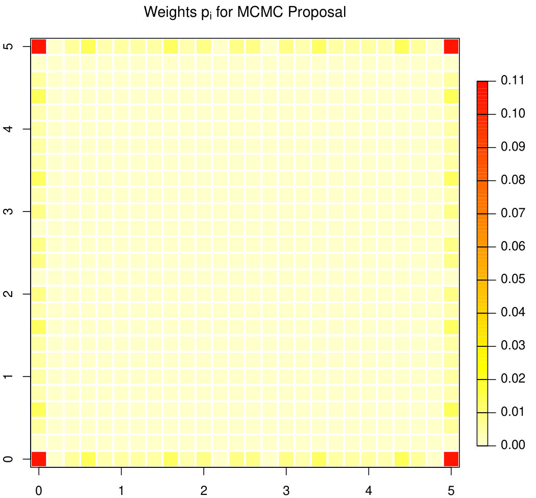 Figure 1
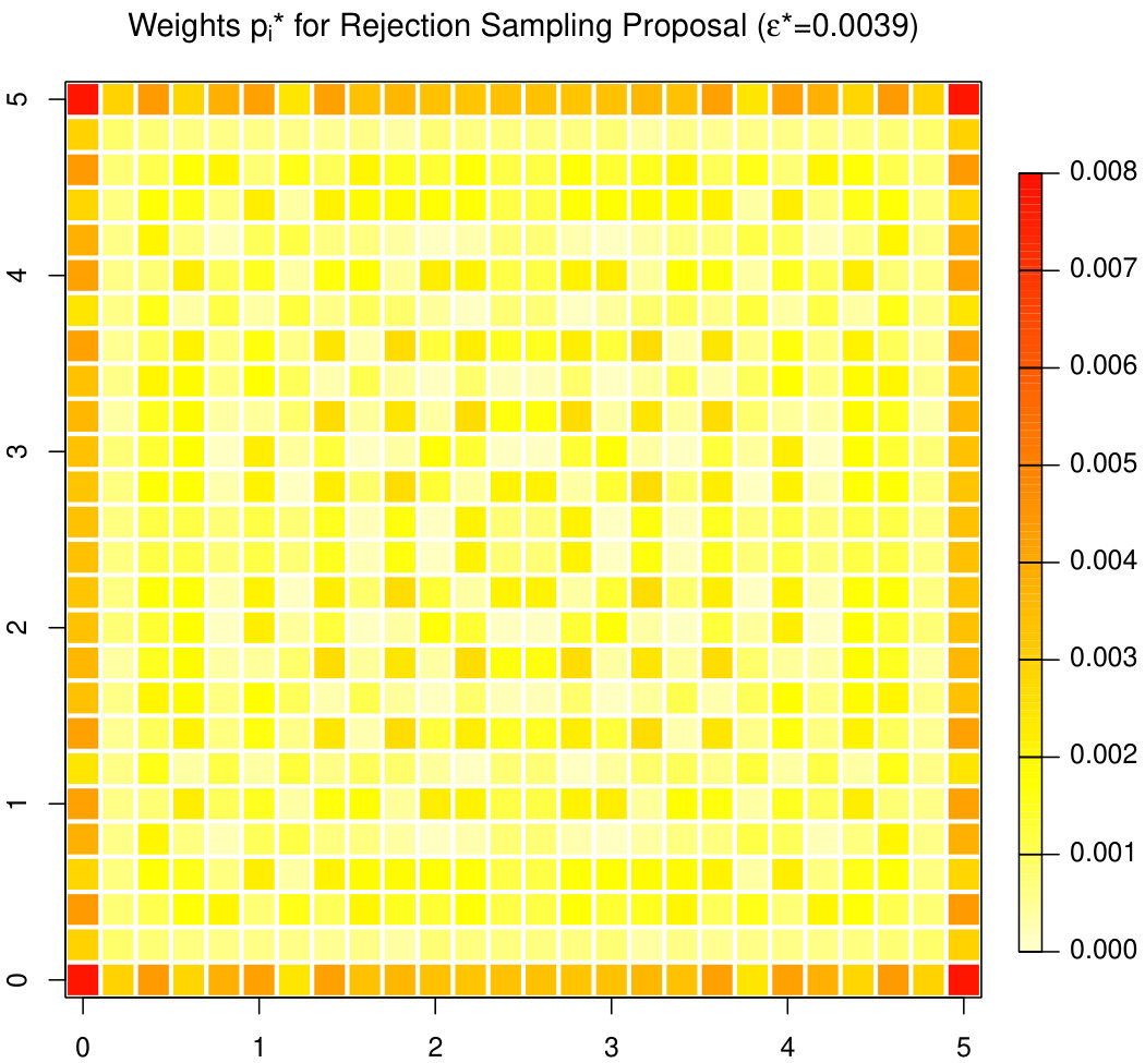 Figure 2
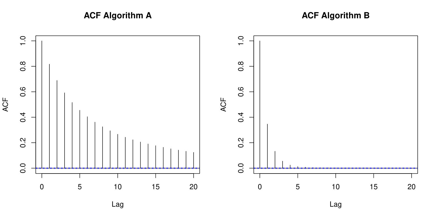 Figure 3
Peer Reviews
No public reviews on file for this paper yet. If you reviewed it on a platform where reviews are public (OpenReview, ICLR, NeurIPS, ICML), you can paste yours below so the community can read it here.
Videos
No videos yet. Explain this paper in a talk, walkthrough, or lecture? Add one.
\historydates\doiheadtext
\authormark
Oesting et al
\corres
*Marco Oesting, Department Mathematik, Universität Siegen, Walter-Flex-Str. 3, D-57072 Siegen, Germany.
Sampling Sup-Normalized Spectral Functions for Brown–Resnick Processes
Marco Oesting
Martin Schlather
Claudia Schillings
\orgdivDepartment Mathematik, \orgnameUniversität Siegen, \orgaddress\countryGermany
\orgdivInstitut für Mathematik, \orgnameUniversität Mannheim, \orgaddress\countryGermany
Abstract
[Summary]Sup-normalized spectral functions form building blocks of max-stable and Pareto processes and therefore play an important role in modeling spatial extremes. For one of the most popular examples, the Brown–Resnick process, simulation is not straightforward. In this paper, we generalize two approaches for simulation via Markov Chain Monte Carlo methods and rejection sampling by introducing new classes of proposal densities. In both cases, we provide an optimal choice of the proposal density with respect to sampling efficiency. The performance of the procedures is demonstrated in an example.
keywords:
Markov Chain Monte Carlo, Max-Stable Process, Pareto Process, Rejection Sampling, Spatial Extremes
1 Introduction
Spatial and spatio-temporal extreme value analysis aims at investigating extremes of quantities described by stochastic processes. In the classical setting, the real-valued process of interest is sample-continuous on a compact domain . Analysis of its extremes is often based on results of the limiting behavior of maxima of independent copies , . Provided that there exist continuous normalizing functions and such that the process of normalized maxima converges in distribution to some sample-continuous process with nondegenerate margins as , the limit process is necessarily max-stable and we say that is in the max-domain of attraction of .
From univariate extreme value theory, it follows that the marginal distributions of are necessarily generalized extreme value (GEV) distributions cf. 4 for instance. As max-stability is preserved under marginal transformations between different GEV distributions, without loss of generality, it can be assumed that has standard Fréchet margins, i.e. , , for all . By de Haan 3, any sample-continuous max-stable process with standard Fréchet margins can be represented as
[TABLE]
where the so-called spectral processes , , are independent copies of a nonnegative sample continuous stochastic process on satisfying for all , and is a Poisson point process on which is independent of the and has intensity measure given by for all .
Due to its complex structure, many characteristics of the max-stable process in (1) cannot be calculated analytically, but need to be assessed via simulations. In order to simulate efficiently, Oesting \BOthers. 15 suggest to make use of the sup-normalized spectral representation
[TABLE]
where the are the same as above, the processes are independently and identically distributed, independently of the , with distribution given by
[TABLE]
and for every , where denotes the set of all real-valued continuous functions on equipped with the supremum norm and corresponding -algebra . Here, the normalizing constant is the so-called extremal coefficient of the max-stable process over the domain . In a simulation study, Oesting \BOthers. 15 demonstrate that simulation based on the sup-normalized spectral representation is competitive to other state-of-the-art algorithms such as simulation based on extremal functions 7 provided that the normalized spectral process can be simulated efficiently.
The law of the processes also occurs when analyzing the extremes of a stochastic process in an alternative way focusing on exceedances over a high threshold: If is in the max-domain of attraction of the max-stable process in (1), we have
[TABLE]
as , where is a standard Pareto random variable and is an independent process with law given in (3). The limit process is called Pareto process cf. 9, 8.
Arising as sup-normalized spectral process for both max-stable and Pareto processes, the process plays an important role in modelling and analyzing spatial extremes. As a crucial building block of spatial and spatio-temporal models, this process needs to be simulated in an efficient way. Due to the measure transformation in (3), however, sampling of is not straightforward even in cases where the underlying spectral process can be simulated easily.
In the present paper, we focus on the simulation of for the very popular class of log Gaussian spectral processes, i.e. for some Gaussian process such that for all . The resulting subclass of max-stable processes in (1) comprises the only possible nontrivial limits of normalized maxima of rescaled Gaussian processes, the class of Brown–Resnick processes 13, 12. In order to obtain Brown–Resnick processes that can be extended to stationary processes on , 13 consider , , with being a centered Gaussian process on with stationary increments and variogram
[TABLE]
It is important to note that the law of the resulting max-stable process does not depend on the variance of , but only on . Therefore, is called Brown–Resnick process associated to the variogram .
Recently, Ho \BBA Dombry 11 introduced a two-step procedure to simulate the corresponding sup-normalized process
[TABLE]
efficiently if the finite domain is of small or moderate size:
Sample the index of the component where the vector assumes its maximum, i.e. select one of the events , . Provided that the covariance matrix of the Gaussian vector is nonsingular, we have that this index is a.s. unique and that the probabilities of the corresponding events can be calculated in terms of the matrix and the vector given by
[TABLE]
where is the variance vector of and . More precisely, by Ho \BBA Dombry 11,
[TABLE]
where denotes the vector after removing the th component, denotes the matrix after removing the th row and th column and is the distribution function of an -dimensional Gaussian distribution with mean vector and covariance matrix evaluated at . 2. 2.
Conditional on , we have and the distribution of the vector is an -dimensional Gaussian distribution with mean vector and covariance matrix conditional on being nonpositive.
However, the first step includes computationally expensive operations such as the evaluation of -dimensional Gaussian distribution functions and the inversion of matrices of sizes and . Furthermore, an efficient implementation of the second step is not straightforward. Thus, the procedure is feasible for small or moderate only.
In this paper, we will introduce alternative procedures for the simulation of , or, equivalently, , that are supposed to work for larger , as well. To this end, we will modify a Markov Chain Monte Carlo (MCMC) algorithm proposed by Oesting \BOthers. 15 and a rejection sampling approach based on ideas of de Fondeville \BBA Davison 2. Both procedures have originally been designed to sample sup-normalized spectral functions in general. Here, we will adapt them to the specific case of Brown–Resnick processes.
2 Simulating via MCMC algorithms
Based on the Brown–Resnick process as our main example, we consider a max-stable process with spectral process for some sample-continuous process . Henceforth, we will always assume that the simulation domain is finite and that the corresponding spectral vector possesses a density w.r.t. some measure on . Then, by (3), the transformed spectral vector , where the logarithm is applied componentwise, has the multivariate density
[TABLE]
which obviously has the same support as , i.e. .
As direct sampling from the density is rather sophisticated and the normalizing constant is not readily available, it is quite appealing to choose an MCMC approach for simulation. In the present paper, we focus on Metropolis-Hastings algorithms with independence sampler cf. 17 for example. Denoting the strictly positive proposal density on by , the algorithm is of the following form:
Algorithm 1**.**
*MCMC APPROACH (METROPOLIS–HASTINGS)
Input: proposal density
Simulate according to the density .
for {
for Sample from and set
for
for where the acceptance probability is given by (4).
}
Output: Markov chain .
Here, the acceptance ratio for a new proposal given a current state is
[TABLE]
using the convention that a ratio is interpreted as [math] if both the enumerator and the denominator are equal to [math]. This choice of ensures reversibility of the resulting Markov chain with respect to the distribution of . Further, it allows for a direct transition from any state to any other state . Consequently, the chain is irreducible and aperiodic and, thus, its distribution converges to the desired stationary distribution, that is, for a.e. initial state , we have that
[TABLE]
where denotes the distribution of the -th state of a Markov chain with initial state and is the total variation norm.
As a general approach for the simulation of sup-normalized spectral processes of arbitrary max-stable processes, Oesting \BOthers. 15 propose to use Algorithm 1 with the density of the original spectral vector as proposal density (Algorithm 1A) and the Metropolis-Hastings acceptance ratio in (4) simplifies to
[TABLE]
As the proposal density is strictly positive on , convergence of the distribution of the Markov chain to the distribution of as in (5) is ensured. If the support of is unbounded, however, there is no uniform geometric rate of convergence of the chain in (5), as we have
[TABLE]
14. In particular, this holds true for the case of a Brown–Resnick process where is a Gaussian vector.
Furthermore, due to the structure of the acceptance ratio in (6), the Markov chain may get stuck, once a state with a large maximum is reached. This might lead to rather poor mixing properties of the chain. Even though independent realizations could still be obtained by starting new independent Markov chains cf. 15, such a behavior is undesirable having chains in high dimension with potentially long burn-in periods in mind.
While the algorithm in Oesting \BOthers. 15 is designed to be applicable in a general framework, we will use a specific transformation to construct a Markov chain with stronger mixing and faster convergence to the target distribution. For many popular models such as Brown–Resnick processes, this transformation is easily applicable. More precisely, we consider the related densities , , with . These densities are closely related to the distributions that have been studied in Dombry \BOthers. 7.
Hence, we propose to approach the target distribution with density by Algorithm 1 using a mixture
[TABLE]
as proposal density, where the weights , , are such that . The corresponding acceptance probability in (4) is then
[TABLE]
With the proposal density being strictly positive on , we can see that the distribution of the Markov chain again converges to its stationary distribution with density . As we further have
[TABLE]
provided that for , the results found by Mengersen \BBA Tweedie 14 even ensure a uniform geometric rate of convergence for any starting value in contrast to the case where .
In order to obtain a chain with good mixing properties, we choose such that the acceptance rate in Algorithm 1 is high provided that the current state is (approximately) distributed according to the stationary distribution. To this end, we minimize the relative deviation between and under , i.e. we minimize
[TABLE]
under the constraint . Introducing a Lagrange multiplier , minimizing
[TABLE]
results in solving the linear system
[TABLE]
where and with
[TABLE]
Provided that the matrix is nonsingular, the solution of (16) is given by
[TABLE]
cf. 1 for instance. This solution does not necessarily satisfy the additional restriction for all . In case that is singular or the vector has at least one negative entry, the full optimization problem
[TABLE]
has to be solved. Using the Karush–Kuhn–Tucker optimality conditions, the quadratic program (2) can be transformed into a linear program with additional (nonlinear) complementary slackness conditions. It can be solved by modified simplex methods. Alternatively, the problem (2) can be solved by the dual method by Goldfarb \BBA Idnani 10.
Remark 2.1**.**
In order to ensure a geometric rate of convergence of the distribution of the Markov chain, we might replace the condition for all in (2) by for some given . Then, a geometric rate of convergence follows from (9) as described above.
In the case of Brown–Resnick processes, for simplicity, we consider the case that possesses a full Lebesgue density. In particular, the covariance matrix of is assumed to be nonsingular. Then, the target density is
[TABLE]
where is again the variance vector of . Now, the densities which form the proposal density are just shifted Gaussian distributions:
[TABLE]
cf. Lemma 1 in the Supplementary Material of Dombry \BOthers. 7, i.e. we have
[TABLE]
where the Gaussian vectors and possess densities and , respectively. The calculation of the optimal weights is based on the expectation in (17) which typically cannot be calculated analytically, but needs to be assessed numerically via simulations. Such a numerical evaluation, however, is challenging as the random variable is unbounded. To circumvent these computational difficulties, we make use of the identity
[TABLE]
This expression can be conveniently assessed numerically as the random variable is bounded by .
Remark 2.2**.**
Note that both (19) and the final result in (20) still hold true if does not possess a full Lebesgue density, but exactly one component is degenerate and the reduced covariance matrix is nonsingular. This situation appears in several examples such as being a fractional Brownian motion where a.s.
In summary, we propose the procedure below to simulate the normalized spectral vector for the Brown–Resnick process (Algorithm 1B):
Calculate by solving the quadratic program (2) where the entries of the matrix are given by (20). Provided that all its components are nonnegative, the solution has the form (18). 2. 2.
Run Algorithm 1 with proposal density and acceptance probability given by (8). The output of the algorithm is a Markov chain whose stationary distribution is the distribution of .
3 Exact Simulation via Rejection Sampling
In this section, we present an alternative procedure to generate samples from with probability density . In contrast to Section 2 where we generated a Markov chain consisting of dependent samples with the desired distribution as stationary distribution, here, we aim to produce independent realizations from the exact target distribution. To this end, we make use of a rejection sampling approach cf. 5 for instance based on a proposal density satisfying
[TABLE]
for some .
Algorithm 2**.**
*REJECTION SAMPLING APPROACH
Input: proposal density and constant satisfying (21)
repeat {
repeat Simulate according to the density .
repeat Generate a uniform random number in .
} until
Output: exact sample from distribution with density
Thus, on average, simulations from the proposal distribution are needed to obtain an exact sample from the target distribution. Of course, to minimize the computational burden, for a given proposal density , the constant should be chosen maximal subject to (21), i.e.
[TABLE]
Recently, de Fondeville \BBA Davison 2 followed a similar idea and suggested to base the simulation of a general sup-normalized spectral process on the relation
[TABLE]
where is a spectral process normalized with respect to another homogeneous functional instead of the supremum norm, i.e. a.s. If is a.s. bounded from above by some constant, from the relation (22), we obtain an inequality of the same type as (21) for the densities of and instead of and , respectively. Thus, samples of can be used as proposals for an exact rejection sampling procedure. For instance, the sum-normalized spectral vector , i.e. the vector which is normalized w.r.t. the functional , can be chosen as it is easy to simulate in many cases cf. 7 and satisfies almost surely.
For a Brown–Resnick process, it is well-known that the sum-normalized process has the same distribution as where has the density from (7) in Section 2 with equal weights see also 6. Thus, in this case, the procedure proposed by de Fondeville \BBA Davison 2 with is equivalent to performing rejection sampling for with as proposal distribution (Algorithm 2A). From Equation (9), it follows that rejection sampling can also be performed with and arbitrary positive weights summing up to , since we have (21) with . Thus, accepting a proposal in the rejection sampling procedure with probability
[TABLE]
we will obtain a sample of independent realizations from the exact target distribution . The rejection rate, however, is pretty high. In order to obtain one realization of , on average simulations from are required. It can be easily seen that the computational costs are indeed minimal for the choice , i.e. the choice in the approach based on the sum-normalized representation. In this case, one realization of on average requires to sample times from . Therefore, this approach becomes rather inefficient if we have a large number of points on a dense grid.
In order to reduce the large computational costs of rejection sampling which are mainly due to the fact that gets small as , we replace each density by the modified multivariate Gaussian density whose variance is increased by the factor for some :
[TABLE]
Analogously to for the MCMC approach in Section 2, we propose a mixture
[TABLE]
with and as proposal density for the rejection sampling algorithm. A proposal is then accepted with probability
[TABLE]
where
[TABLE]
Thus, to summarize, for appropriately chosen and such that , we propose to run Algorithm 2 with proposal density and according to (3).
Remark 3.1**.**
To further reduce the computational costs in the simulation, we might even choose a more flexible approach. For instance, instead of using a mixture of a finite number of functions , one could consider arbitrary mixtures
[TABLE]
where on the enlarged domain and is a probability measure on . Furthermore, depending on , different values for might be chosen. However, due to the complexity of the optimization problems involved, we restrict ourselves to the situation above where is a probability measure on and is constant in space.
Using the procedure described above, on average, simulations from the proposal distribution are needed to obtain one exact sample from the target distribution, i.e. the computational complexity of the algorithm depends on the choices of and . The remainder of this section will be devoted to this question.
Choice of and
For a given , the computational costs of the algorithm can be minimized by choosing such that the constant given in (3) is maximal, i.e. by choosing as the solution of the nonlinear optimization problem
[TABLE]
Optimizing further w.r.t. , we obtain the optimal choice where .
As the above optimization problem includes optimization steps w.r.t. , and , none of which can be solved analytically, the solution is quite involved. In order to reduce the computational burden, we simplify the problem by maximizing an analytically simpler lower bound. To this end, we decompose the convex combination into sums over disjoint subsets of the form . For a convex combination of with weight vector , we obtain the lower bound
[TABLE]
where we made use of the convexity of the exponential function. Setting , this bound can be calculated explicitly:
[TABLE]
Hence,
[TABLE]
where for every subset . Now, for each , let be a partition of , so that
[TABLE]
Thus, the RHS of (3) provides an explicit lower bound for the average acceptance probability for any choice of the .
Remark 3.2**.**
Assume that, for some , there is some index set such that for all . Then, Equation (3) provides the bound
[TABLE]
for all . Alternatively, for the same index set , we could bound each summand separately, i.e.
[TABLE]
Note that, for all , the RHS of (28) is less than the RHS of (27), i.e. the lower bound is less sharp. Therefore, we prefer pooling locations with the same distance to rather than considering them separately in order to have the bound in (3) as sharp as possible.
In view of (3), instead of considering the exact value which is needed to calculate the minimal rejection rate, but cannot be given explicitly, we might maximize the function
[TABLE]
for fixed partitions . Due to the complex dependence of on , the resulting optimization problem is nonlinear in even for fixed . To circumvent this difficulty, for each , we fix -dimensional weight vectors and consider the function
[TABLE]
with and for the unique set such that .
Analogously to the solution above, we first maximize for fixed and , i.e. we consider the optimization problem
[TABLE]
To convert the linear program to standard form, we introduce an additional variable , unconstrained in sign, leading to the equivalent program
[TABLE]
The standard form of (3) is then given by
[TABLE]
Such a linear program in standard form can be solved by standard techniques such as the simplex algorithm. Compared to the optimization of , the complementary one-dimensional problem of maximizing for fixed can be solved rather easily.
To summarize, starting from some and , we propose to apply the following two steps repeatedly (Algorithm 2B):
Define
[TABLE]
and set
[TABLE]
i.e. the solution of the optimization problem (3) (or (3) or (3), equivalently). 2. 2.
Set .
Even though might be significantly smaller than , in some cases, this bound is already sufficient to improve the results for that have been discussed in the beginning of this section, where we have already seen that the corresponding optimal weight vector equals and that . We show an example to illustrate that this choice is not necessarily optimal, i.e. there is some and a vector of weights such that .
Example 3.3** (Fractional Brownian Motion).**
Let be equidistant locations in and for some . Choose , and set . Then, for every there are at least locations such that . Thus, we obtain for large that
[TABLE]
which is eventually larger than as .
4 Illustration
Finally, we illustrate the performance of Algorithm 1 and the rejection sampling algorithm in an example. Taking up Example 3.3 in higher dimension, we consider the case that is a Brown–Resnick process associated to the variogram
[TABLE]
on the grid ( points). We run four different algorithms:
- 1A.
Algorithm 1 with proposal density as proposed by Oesting \BOthers. 15 2. 1B.
Algorithm 1 with proposal density where is given as the solution of (2) (cf. Section 2). 3. 2A.
Algorithm 2 with proposal density and (equivalent to the procedure proposed in de Fondeville \BBA Davison 2 based on sum-normalized spectral functions) 4. 2B.
Algorithm 2 with proposal density and in (3) where and are obtained as described in Section 3
Even though the laws of the Brown–Resnick process and the normalized spectral process do not depend on the variance, but only on the variogram of the underlying Gaussian process , the choice of the Gaussian process may affect the performance of the algorithms. Here, we choose the Gaussian process whose law is uniquely defined via the construction
[TABLE]
where is an arbitrary centered Gaussian process with variogram . Oesting \BBA Strokorb 16 show that this process has a smaller maximal variance and is thus preferable in the context of simulation.
We first calculate the optimal weights as a solution of (2) (used in Algorithm 1B) as well as the optimal weights as a solution of (3) and the optimal variance modification (used in Algorithm 2B). The results for and are displayed in Figure 1. It can be seen that, in both cases, the weights are not spatially constant, but are larger on the boundary of the convex hull with the maximum in the corners of the square. This observation is well in line with the fact that these points have the largest contribution to since the variance of attains its maximum there see also 16.
We run Algorithm 1 with both proposal densities as specified above (Algorithms 1A and 1B, respectively) to obtain two Markov chains and of length . It can be seen that the empirical acceptance rate of the second chain () is remarkably higher than the one of the first chain () which already indicates stronger mixing. This impression is confirmed by analyzing the empirical autocorrelation functions of the time series and which are shown in Figure 2. Here, the empirical autocorrelation in the second chain is drastically reduced in comparison with the first chain, indicating that two states of the chain can be regarded as nearly uncorrelated after roughly five steps.
The rejection sampling algorithm (Algorithm 2A and Algorithm 2B) automatically generates independent realizations from the multivariate target density . Therefore, we will compare them with respect to their computational complexity. To this end, we run them to generate a sample of size and count the average number of simulations of Gaussian vectors from the proposal density to generate one realization of . In case of Algorithm 2A, this number is which is close to the theoretical expression . For Algorithm 2B, the number is improved by a factor of approximately , leading to an average number of Gaussian vectors to be simulated to obtain one realization from the target distribution. This improvement is well in line with the corresponding value .
As the example illustrates, the two modifications we suggested may lead to significant improvements of MCMC and rejection algorithms that have been proposed so far. Here, only the modified rejection sampling algorithm ensures independence of exact samples from the target distribution. However, as the example indicates, the MCMC algorithm might be particularly attractive in practice as a thinned chain results in nearly independent samples even if the thinning rate is rather small. Note that we also tried other examples such as a Brownian sheet (). However, we found that significant improvements in the rejection sampling procedure become apparent only for , see also Example 3.3.
Acknowledgements
The authors are grateful to Kirstin Strokorb, Dimitri Schwab and Jonas Brehmer for numerous valuable comments. M. Schlather has been financially supported by Volkswagen Stiftung within the project ‘Mesoscale Weather Extremes – Theory, Spatial Modeling and Prediction (WEX-MOP)’.
The reference list from the paper itself. Each links out to its DOI / PubMed record.
- 1Cressie \APA Cyear 1993 \APA Cinsertmetastar cressie 93 {APA Crefauthors} Cressie, N \BPBI A. \APA Cref Year 1993. \APA Crefbtitle Statistics for Spatial Data Statistics for Spatial Data. \APA Caddress Publisher New York John Wiley & Sons. \Print Back Refs \Current Bib
- 2de Fondeville \BBA Davison \APA Cyear 2018 \APA Cinsertmetastar d FD 17 {APA Crefauthors} de Fondeville, R. \BCBT \BBA Davison, A \BPBI C. \APA Cref Year Month Day 2018. \BBOQ \APA Crefatitle High-dimensional peaks-over-threshold inference High-dimensional peaks-over-threshold inference. \BBCQ \APA Cjournal Vol Num Pages Biometrika 1053575-592. \Print Back Refs \Current Bib
- 3de Haan \APA Cyear 1984 \APA Cinsertmetastar dehaan-84 {APA Crefauthors} de Haan, L. \APA Cref Year Month Day 1984. \BBOQ \APA Crefatitle A spectral representation for max-stable processes A spectral representation for max-stable processes. \BBCQ \APA Cjournal Vol Num Pages Ann. Probab.1241194–1204. \Print Back Refs \Current Bib
- 4de Haan \BBA Ferreira \APA Cyear 2006 \APA Cinsertmetastar dhf 06 {APA Crefauthors} de Haan, L. \BCBT \BBA Ferreira, A. \APA Cref Year 2006. \APA Crefbtitle Extreme Value Theory: An Introduction Extreme Value Theory: An Introduction. \APA Caddress Publisher New York Springer. \Print Back Refs \Current Bib
- 5Devroye \APA Cyear 1986 \APA Cinsertmetastar devroye-1986 {APA Crefauthors} Devroye, L. \APA Cref Year 1986. \APA Crefbtitle Non-Uniform Random Variate Generation Non-Uniform Random Variate Generation. \APA Caddress Publisher New York Springer-Verlag. \Print Back Refs \Current Bib
- 6Dieker \BBA Mikosch \APA Cyear 2015 \APA Cinsertmetastar dieker-mikosch-15 {APA Crefauthors} Dieker, A \BPBI B. \BCBT \BBA Mikosch, T. \APA Cref Year Month Day 2015. \BBOQ \APA Crefatitle Exact simulation of Brown-Resnick random fields at a finite number of locations Exact simulation of Brown-Resnick random fields at a finite number of locations. \BBCQ \APA Cjournal Vol Num Pages Extremes 182301–314. \Print Back Refs \Current Bib
- 7Dombry \B Others . \APA Cyear 2016 \APA Cinsertmetastar deo 16 {APA Crefauthors} Dombry, C., Engelke, S. \BCBL \BBA Oesting, M. \APA Cref Year Month Day 2016. \BBOQ \APA Crefatitle Exact Simulation of Max-Stable Processes Exact simulation of max-stable processes. \BBCQ \APA Cjournal Vol Num Pages Biometrika 1032303–317. \Print Back Refs \Current Bib
- 8Dombry \BBA Ribatet \APA Cyear 2015 \APA Cinsertmetastar dombry-ribatet-15 {APA Crefauthors} Dombry, C. \BCBT \BBA Ribatet, M. \APA Cref Year Month Day 2015. \BBOQ \APA Crefatitle Functional regular variations, Pareto processes and peaks over threshold Functional regular variations, Pareto processes and peaks over threshold. \BBCQ \APA Cjournal Vol Num Pages Stat. Interface 819–17. \Print Back Refs \Current Bib