Stability for a second type partitioning problem
Jinyu Guo, Chao Xia

TL;DR
This paper investigates the stability properties of type-II partitioning problems, classifying stable hypersurfaces in space forms, providing topological restrictions in convex domains, and establishing Morse index bounds based on topology.
Contribution
It offers a complete classification of stable type-II stationary hypersurfaces in space forms and topological restrictions for surfaces in convex domains, along with Morse index bounds.
Findings
Stable hypersurfaces are totally geodesic n-balls in space forms
Topological restrictions for stable surfaces in convex domains
Lower bounds for Morse index based on topology
Abstract
In this paper, we study stability and instability problem for type-II partitioning problem. First, we make a complete classification of stable type-II stationary hypersurfaces in a ball in a space form as totally geodesic -balls. Second, for general ambient spaces and convex domains, we give some topological restriction for type-II stable stationary immersed surfaces in two dimension. Third, we give a lower bound for the Morse index for type-II stationary hypersurfaces in terms of their topology.
Click any figure to enlarge with its caption.
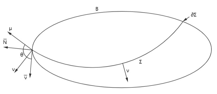 Figure 1
Peer Reviews
No public reviews on file for this paper yet. If you reviewed it on a platform where reviews are public (OpenReview, ICLR, NeurIPS, ICML), you can paste yours below so the community can read it here.
Videos
No videos yet. Explain this paper in a talk, walkthrough, or lecture? Add one.
Stability for a second type partitioning problem
Jinyu Guo
School of Mathematical Sciences
Xiamen University
361005, Xiamen, P.R. China
and
Chao Xia
School of Mathematical Sciences
Xiamen University
361005, Xiamen, P.R. China
Abstract.
In this paper, we study stability and instability problem for type-II partitioning problem. First, we make a complete classification of stable type-II stationary hypersurfaces in a ball in a space form as totally geodesic -balls. Second, for general ambient spaces and convex domains, we give some topological restriction for type-II stable stationary immersed surfaces in two dimension. Third, we give a lower bound for the Morse index for type-II stationary hypersurfaces in terms of their topology.
MSC 2010: 53A10, 53C24, 53C40.
Keywords: Partitioning problem, Minimal surfaces, Capillary surfaces, Stability, Rigidity.
This work is supported by NSFC (Grant No. 11871406), the Natural Science Foundation of Fujian Province of China (Grant No. 2017J06003) and the Fundamental Research Funds for the Central Universities (Grant No. 20720180009).
Contents
-
3 Uniqueness for type-II stable stationary hypersurfaces in a ball
-
4 Topological restriction on type-II stable stationary surface
1. Introduction
Let be a convex body (compact convex set with non-empty interior). We look at hypersurfaces in which divides into to two disjoint domains and in different manners. In the literature the following two types of partitioning problems have been considered.
Type-I partitioning problem. Find the area-minimizing hypersurfaces among all hypersurfaces in which divides into two disjoint domains and with prescribed volume, namely,
[TABLE]
Type-II partitioning problem. Find the area-minimizing hypersurfaces among all such hypersurfaces in which divides into two disjoint domains and with prescribed wetting boundary area111wetting boundary means for the boundary part on . The word “wetting” comes from the physical model of capillary surfaces., namely,
[TABLE]
These two problems haven been intensively studied by Burago-Maz’ya in late 60s [10] in the case , the unit ball. By using spherical symmetrization, they showed that the solution for Type-I partitioning problem is totally geodesic -ball and all spherical caps intersecting orthogonally (see [20], Section 5.2.1, Lemma 1), while the solution for Type-II partitioning problem is all totally geodesic -balls (see [20], Section 9.4.4, Lemma). Bokowsky-Sperner [9] also studied these two partitioning problems and gave the same classification result as Burago-Maz’ya when is a ball. They also gave several estimates for the corresponding isoperimetric ratio when is a general convex body.
Besides the area-minimizing hypersurfaces, one is also interested in studying stationary hypersurfaces for these partitioning problems. It follows from the first variational formulas (see e.g. Section 2) that stationary hypersurfaces for Type-I partitioning problem are free boundary constant mean curvature (CMC) hypersurfaces, while stationary hypersurfaces for Type-II partitioning problem are minimal hypersurfaces intersecting at a constant angle. Here free boundary means the hypersurfaces intersects orthogonally. There have been plenty of works about existence, regularity and construction of free boundary CMC hypersurfaces, especially free boundary minimal hypersurfaces in the last four decades.
When is a ball, there are several rigidity results, for example, Hopf type theorem by Nitsche [21] and Ros-Souam [25], Alexandrov type theorem by Ros-Souam [25] for these two types stationary hypersurfaces. In particular, it has been found by Fraser-Schoen’s series of works [14, 15, 16] that free boundary minimal hypersurfaces in a ball turns out to have close relationship with the Steklov eigenvalue problem.
Stability problem for Type-I partitioning problem has been initiated and studied by Ros-Vergasta [26]. A free boundary CMC hypersurface is called type-I stable if the second variation of the area functional at this hypersurface is non-negative among any volume-preserving variations. Type-I stable free boundary CMC hypersurfaces are smooth local minimizers for Type-I partitioning problem. In the framework of sets of finite perimeter, the local minimizers for Type-I partitioning problem have been considered by Sternberg-Zumbrun [30] in 1998. It has been conjectured that the free boundary totally geodesic -ball and free boundary spherical caps are all type-I stable free boundary CMC hypersurfaces in . This conjecture has been recently solved by Nunes [22] in two dimension (see also Barbosa [5]) and Wang-Xia [32] in any dimensions. Moreover, Wang-Xia [32] also gave complete classification for type-I stable capillary hypersurfaces in , namely, CMC hypersurfaces intersecting at a constant contact angle.
The first aim of this paper is to study stability problem for type-II partitioning problem. Recall that stationary hypersurfaces for type-II partitioning problem in are minimal hypersurfaces intersecting at a constant angle. We call a minimal hypersurfaces intersecting at a constant angle is type-II stable if the second variation of the area functional at this hypersurface is non-negative among any wetting-area-preserving variations. We show the following complete classification for type-II stable minimal hypersurfaces in intersecting at a constant angle.
Theorem 1.1**.**
A type-II stable stationary immersed hypersurface in an Euclidean ball is a totally geodesic -ball.
In case that the ball lies in a space form, we have the similar result.
Theorem 1.2**.**
A type-II stable stationary immersed hypersurface in a (n+1)-ball in a space form is a totally geodesic -ball.
For general convex bodies in general ambient -manifolds, we obtain some topological restriction for type-II stable stationary immersed surfaces.
Theorem 1.3**.**
Let be a type-II stable stationary compact immersed surface with free boundary. Assume and . Then the only possible values for the genus and the number of boundary component of are and or and . Moreover, and happens only when along and along .
Theorem 1.4**.**
Let be a type-II stable stationary compact immersed surface. Assume and . Assume is embedded in . Then the only possible values for the genus and the number of boundary component of are if is even and if is odd.
In Theorems 1.3 and 1.4, , and denote the sectional curvature, the Ricci curvature and the scalar curvature of respectively, and denotes the second fundamental form of .
The instability for a variational problem is quantitatively measured by the Morse index. For the type-II partitioning problem, the Morse index for a stationary hypersurface is the non-negative integer which indicates the dimension of sets of wetting-area-preserved deformations which decreases the area of the type-II stationary hypersurface. A stationary hypersurface is stable is equivalent that it has vanishing Morse index. It turns out that the Morse index controls the topology and geometry for stationary hypersurfaces.
There are plenty of works on the index estimate for closed minimal hypersurfaces or minimal hypersurfaces with free boundary, see for example, Ros [24], Savo [29] and Ambrozio-Carlotto-Sharp [3, 4]. See also [23, 12, 13] for index estimate for CMC surfaces with free boundary, which is related to type-I partitioning problem. The technique in [23, 12, 13] for non-minimal CMC case only applies for two dimension.
The next aim of this paper is to study the index estimate for minimal hypersurfaces with constant contact angle, i.e., stationary hypersurfaces for type-II partitioning problem. We use to denote the Morse index for a type-II stationary hypersurface . Following the argument of Savo [29] and Ambrozio-Carlotto-Sharp [3, 4], by using the coordinates of harmonic one-forms, we are able to prove the following lower bound for the index.
Theorem 1.5**.**
Let be a type-II stationary compact immersed hypersurface. Let be isometrically embedded in . Assume for any non-zero vector field on satisfies
[TABLE]
where and denote the Riemannian curvature tensor and Ricci curvature tensor of respectively, denotes the mean curvature of , and denotes the second fundamental form for the embedding . Then
[TABLE]
where denotes the first relative homology group with real coefficients.
As a corollary, we have the following
Corollary 1.1**.**
Let be a strictly mean convex domain in and be a type-II stationary compact immersed hypersurface. Then
[TABLE]
Using another argument of Ros [23] and Ambrozio-Carlotto-Sharp [3], again using the coordinates of harmonic one-forms, we can get the following Morse index estimate for two dimension.
Theorem 1.6**.**
Let be a type-II stationary compact immersed surface. Let be isometrically embedded in . Assume for any non-zero vector field on satisfies
[TABLE]
Then
[TABLE]
In the case of and is mean convex domain, the inequality (1.2) is satisfied. (In the case , one needs use the fact that there are no minimal closed surfaces in ). Therefore we have the following corollaries.
Corollary 1.2**.**
Let be a mean convex domain in and be a type-II stationary compact immersed surface. Then
[TABLE]
Corollary 1.3**.**
Let be a mean convex domain in and be a type-II stationary compact immersed surface. Then
[TABLE]
The remaining part of this paper is organized as follows. In Section 2 we review the definition and basic properties of type-II stationary hypersurfaces. In Section 3 we give a proof of Theorem 1.1 for type-II stationary hypersurfaces in a ball in after finding admissible test function (3.2). and we will provide a detailed proof of Theorem 1.2 for type-II stationary hypersurfaces in a ball in and sketch a proof for type-II hypersurfaces in a ball in . In Section 4, we use balancing argument to study stability problem for type-II stationary hypersurfaces in general convex bodies in general ambient manifolds, and prove Theorem 1.3 and 1.4. In Section 5, we give Morse index estimate lower bounds for type-II stationary hypersurfaces, and prove Theorems 1.5 and 1.6,
2. Preliminaries
Let be an oriented -dimensional Riemannian manifold and be a smooth compact domain in that is diffeomorphic to an Euclidean ball. Let be an isometric immersion of an orientable -dimensional compact manifold with boundary into satisfying
[TABLE]
Such an immersion is called proper.
We denote by , and the gradient, the Laplacian and the Hessian on respectively, while by , and the gradient, the Laplacian and the Hessian on respectively. We will use the following terminology for four normal vector fields. We choose one of the unit normal vector field along and denote it by . We denote by the unit outward normal to in and be the unit outward normal to in . Let be the unit normal to in such that the bases and have the same orientation in the normal bundle of . Denote by and the second fundamental form and the mean curvature of the immersion respectively. Precisely, and
By an admissible variation of , we mean a differentiable map such that is an immersion satisfying and for every and . We denote the area functional of the immersion by
[TABLE]
where is the volume element of in the metric induced by . We denote the wetting area functional are defined by
[TABLE]
where is the area element of . A variation is said to be wetting-area-preserving if for each .
It is easy to see that the first variation formulae of and for an admissible variation with a variation vector field are given by
[TABLE]
where and are the area element of and respectively.
Definition 2.1**.**
A proper immersion is said to be type-II stationary if for any wetting-area-preserving variation of .
From the above first variation formulae, we know that is type-II stationary if and only if is a minimal immersion, namely , and
[TABLE]
Equation (2.3) implies intersects at some constant angle such that .
We make a choice of the normal so that, along , the angle between and or equivalently between and is everywhere equal to (see Figure 1). To be more precise, in the normal bundle of , we have the following relations:
[TABLE]
For , from (2.5) and the fact , we see that a wetting-area-preserving variation with , where is the tangential part of , satisfies
[TABLE]
Conversely, we shall show
Proposition 2.1**.**
Let be a proper type-II stationary immersion with a contact angle . Then for a given satisfying , there exists an admissible wetting-area-preserving variation of with variational vector field having as its normal part.
Proof.
We first assume is embedded. For each point , let be the projection of on . Denote which is tangential to along . Extend smoothly to a vector field on , still denote by . Denote and extend smoothly to a vector field on , which is a -neighborhood of in , such that is tangential to along . By construction, . Consider the local flow of in , that is, . Let be given by . We shall find a function such that
[TABLE]
is the desired deformation. First, since is the local flow of and is tangential to along , we know . Second, since
[TABLE]
where we have
[TABLE]
Let be the local solution of the following initial value problem:
[TABLE]
It follows from the condition that that is, is a wetting area preserving admissible deformation. Finally, it is easy to see that
[TABLE]
which means the variational vector field of has as its normal part.
In the general case of immersion, we shall first construct an admissible variation and endow with the pull-back metric and it is enough to prove the result for endowed with , which is the embedded case. See [2], Proposition 2.1 for details. ∎
The second variational formula of the area functional under admissible wetting-area-preserving variations is given as follows.
Proposition 2.2**.**
Let be a proper type-II stationary immersion. Let be an admissible wetting-area-preserving variation with variational vector field having as its normal part. Then
[TABLE]
Here
[TABLE]
* is the Ricci curvature tensor of , and is that of in given by .*
We postpone the proof of Proposition 2.2 to Appendix A.
Definition 2.2**.**
A proper type-II stationary immersion is called stable if for all wetting-area-preserving variations, that is,
[TABLE]
for any satisfying . Here is as in (2.8).
3. Uniqueness for type-II stable stationary hypersurfaces in a ball
3.1. The Euclidean case
In this subsection, we consider the case and is the Euclidean unit ball (in our notation, is the Euclidean unit open ball). In this case, , and . Abuse of notation, we use to denote the position vector in . We use to denote the Euclidean inner product.
The stability condition becomes
[TABLE]
with
[TABLE]
for all such that .
Theorem 3.1**.**
A type-II stable minimal hypersurfaces in intersecting at a constant angle is a totally geodesic -ball.
Proof.
For convenience, we omit writing the volume form and the area form in an integral.
We know that is minimal and intersects at a constant angle, say . For each constant vector field , Define on ,
[TABLE]
By direct computation, by using (2.4) and (2.5), one sees
[TABLE]
On the other hand, since is minimal, we have
[TABLE]
Thus, by integration by parts, we see
[TABLE]
Therefore, is an admissible test function in (3.1). It follows that
[TABLE]
We can compute that on by [32] Proposition 2.1,
[TABLE]
Also, on ,
[TABLE]
Thus
[TABLE]
Using (3.4) and (3.5) in (3.3), we get that for each ,
[TABLE]
We take to be the coordinate vectors in , and add (3.6) for all to get
[TABLE]
Let , we know that from (2.5). Thus
[TABLE]
and combining with (3.7), we have
[TABLE]
On the other hand, we have
[TABLE]
It follows that
[TABLE]
Thus, inequality (3.8) reduces to
[TABLE]
We conclude that which implies that is a totally geodesic -ball in . ∎
3.2. The hyperbolic case
Let be the simply connected hyperbolic space with curvature . We use here the Poincaré ball model, which is given by
[TABLE]
In this subsection we use or to denote the Euclidean metric and the Cartesian coordinate in . Sometimes we also represent the hyperbolic metric, in terms of the polar coordinate with respect to the origin, as
[TABLE]
We use to denote the hyperbolic distance from the origin and denote . It is easy to verify that
[TABLE]
The position function , in terms of polar coordinate, can be represented by
[TABLE]
It is well-known that is a conformal Killing vector field with
[TABLE]
Let be a ball in with hyperbolic radius . By an isometry of , we may assume is centered at the origin. , when viewed as a set in , is the Euclidean ball with radius . The principal curvatures of are . The unit normal to with respect to is given by
[TABLE]
Moreover, for each constant vector field , we can define a smooth vector field in by
[TABLE]
From [32] Proposition 4.1, we know that is a Killing vector field in , i.e.,
[TABLE]
Denote function as follow
[TABLE]
Proposition 3.1**.**
[32]** For any tangential vector field on , we have
[TABLE]
Proposition 3.2**.**
Let be an isometric immersion into the hyperbolic ball with zero mean curvature , whose boundary intersects at a constant angle . For each constant vector field define
[TABLE]
Then satisfies
[TABLE]
Along , we have
[TABLE]
where
[TABLE]
Proof.
In this proof we always take value along and use (2.4) and (2.5). Firstly, from (3.15) we get
[TABLE]
On the other hand, using integration by parts, we see
[TABLE]
Combining (3.25) with (3.26), we get
[TABLE]
Applying (2.4), (2.5) and (3.13), we have
[TABLE]
Using (3.27) and (3.28), we get the first equation (3.22).
Next, note that
[TABLE]
Therefore,
[TABLE]
By (3.16), (3.17) and [32] Proposition 2.1, we can compute that
[TABLE]
Using and , we obtain
[TABLE]
Therefore, applying relationship , we have
[TABLE]
By (3.28), we complete this proposition. ∎
Theorem 3.2**.**
Assume is an immersed type-II stable hypersurface in the ball with zero mean curvature and constant contact angle . Then is totally geodesic.
Proof.
The stability inequality (2.7) reduces to
[TABLE]
for all function , where is given by (3.24) since has constant principal curvature .
For each constant vector field , we consider
[TABLE]
along .
Equation (3.22) tells us that . Therefore, is an admissible function for testing stability.
Using (3.19) and (3.20), noting that and (3.29), we compute that
[TABLE]
Therefore, we have
[TABLE]
and in turn
[TABLE]
From (3.23), we know
[TABLE]
Inserting (3.32) and (3.33) into the stability condition (3.31), we get for any ,
[TABLE]
We take to be the coordinate vectors in . Noticing that , , we have
[TABLE]
Therefore, by summing (3.34) for all , we get
[TABLE]
As in the Euclidean case, we introduce an auxiliary function
[TABLE]
From (3.18) and , we get
[TABLE]
Note that . Thus we have
[TABLE]
Adding this to (3.35), using (3.36), we have
[TABLE]
This implies is totally geodesic. The proof is completed. ∎
3.3. The spherical case
In this subsection, we sketch the necessary modifications in the case that the ambient space is the spherical space form . We use the model
[TABLE]
to represent , the unit sphere without the south pole. Let be a ball in with radius centered at the north pole. The corresponding . the Killing vector field in this case are
[TABLE]
The crucial functions and in this case are
[TABLE]
Similarly as the hyperbolic case, these functions span the vector space
[TABLE]
Using , , and , the proof goes through parallel to the hyperbolic case. The method works for balls with any radius . Compare to the hyperbolic case, in this case can be negative when . Nevertheless, by going through the proof, we see this does not affect the issue on stability. ∎
4. Topological restriction on type-II stable stationary surface
In this section, we use two kinds of balancing arguments, similar to Ros-Vergasta [26] and Nunes [22], to get topological restriction on type-II stable stationary surfaces.
Step 1. Let be a compact Riemann surface obtained from by attaching a conformal disk at any connected component of . Then there exists a non-trivial conformal map such that (see [31] p. 261)
[TABLE]
Let be the restriction of to . Then be a conformal immersion. By Hersch [18] and Li-Yau [19]’s result, by combining with a conformal diffeomorphism of , we can assume
[TABLE]
where denotes the coordinate function of in .
Using as admissible test functions in (2.9), we get
[TABLE]
Summing up the above inequalities for , using we get
[TABLE]
By conformality of , we have
[TABLE]
Using the Gauss equation and the Gauss-Bonnet formula, taking into account that , we have
[TABLE]
Here is the geodesic curvature of in and is the Gauss curvature of . It follows that
[TABLE]
On the other hand, from (2.4) and (2.5), we have
[TABLE]
Thus
[TABLE]
where . In turn,
[TABLE]
Taking into account of (4.2), (4.3), (4.4) in (4.1), we have
[TABLE]
Step 2. By a result of Ahlfors [1] and Gabard [17], there exists a conformal branched cover such that
[TABLE]
on . Also, by combining with a conformal diffeomorphism of , we can assume
[TABLE]
Thus are admissible test functions in (2.9). We obtain
[TABLE]
By conformality of , we have
[TABLE]
Using the same argument as Step 1, we get
[TABLE]
Proof of Theorem 1.3
Consider the free boundary case, i.e. . In this case one has
[TABLE]
Hence, from (4.5) and (4.8), by our assumption that and , we deduce that and , or and . Moreover, and happens only when along and along .
Proof of Theorem 1.4
Let us consider the general case, . Assume is embedded. Then divide by several components.We choose one of these components, denoted by , so that intersects with . We know
[TABLE]
Then
[TABLE]
By the Gauss-Bonnet formula for , we have
[TABLE]
Hence
[TABLE]
Note that depending on the choice of . By the Gauss equation, if and , we know the Gauss curvature of is nonnegative and in turn,
[TABLE]
Using (4.5), we conclude that and .
5. Morse index estimate
In this section, we will discuss lower bound estimates for Morse Index of stationary type-II hypersurface in a connected domain in .
For any , we set
[TABLE]
Here is as in (2.8).
Definition 5.1**.**
Let be a type-II stationary immersed hypersurface. The Morse index of is defined to be the maximal dimension of a subspace of such that
[TABLE]
For the Jacobi operator , with the boundary condition
[TABLE]
there exists a non-decreasing and diverging sequence of eigenvalues associated to a -orthonormal basis of solutions to the eigenvalue problem
[TABLE]
By Rayleigh’s theorem, the eigenvalues has the following variational characterization
[TABLE]
where and is the orthogonal complement of with respect to the inner product of .
The Morse index of a type-II stationary hypersurface is closely related to the number of negative eigenvalues of (5.1). For type-I case, a similar statement can be found in the literature, see e.g. [8, 28].
Proposition 5.1**.**
Let be the number of negative eigenvalues of (5.1). Then
[TABLE]
Proof.
Let be the subspace consisting of the first eigenfunctions for (5.1). Since
[TABLE]
we have and
On the other hand, consider the linear operator defined by
[TABLE]
It follows that
[TABLE]
∎
Thanks to above proposition, to estimate the Morse index of , one only needs to estimate the number of negative eigenvalues of (5.1). Next we use the method of Savo [29], Ambrozio-Carlotto-Sharp [3, 4] to find an estimate of number of negative eigenvalues of (5.1) in terms of topological invariant.
First, let be isometrically embedded in . Let be a canonical basis of . We use to denote the inner product of and to denote the covariant derivative of . We use to denote the second fundamental form for the embedding Given a vector field on , we denote by its dual 1-form.
5.1. First method: coordinates of
Define
[TABLE]
where is the outward unit normal vector field of . Then we have the following key formula.
Proposition 5.2**.**
Let
[TABLE]
Then
[TABLE]
where is an orthonormal basis of .
Proof.
The proof is close to Savo [29], Ambrozio-Carlotto-Sharp [4], small difference arises from the boundary computation. We prove it here for reader’s convenience. A direct computation gives
[TABLE]
Note that
[TABLE]
It follows that
[TABLE]
and in turn
[TABLE]
Using the Gauss equation for the immersion , taking account , we have
[TABLE]
Note that . It follows that
[TABLE]
By the Weintzenböck formula, using that , we have
[TABLE]
On the other hand, by choosing is orthonormal basis of , we get
[TABLE]
Since along , then along for some smooth function on . Thus
[TABLE]
Combining the above computation, we get
[TABLE]
Recall that
[TABLE]
Thus
[TABLE]
It follows that
[TABLE]
where in the last equality we used . We get the assertion (5.2). ∎
Proof of Theorem 1.5. Assume the number of negative eigenvalues of (5.1) is . Define
[TABLE]
where are functions defined via by (5.2) and ranges from to and ranges from to .
First, we claim that
For any non-zero 1-form , this means that , thus
[TABLE]
by the variational characterization of the eigenvalue problem (5.1). In particular, by (5.2) and hypothesis (1.5), we have
[TABLE]
Hence has trivial kernel.
Next, we observe that is a linear operator and
[TABLE]
Thus
[TABLE]
By [4] Theorem 3, we have the following isomorphisms
[TABLE]
Recall from Proposition 5.1 that . The assertion follows. ∎
Remark 5.1**.**
The dimension of this homology group can be explicitly computed in terms of the homology groups of and (see [4], Lemma 4).
5.2. Second method: coordinates of
Now we consider case. Assume is type-II stationary surface in . Given a vector field on , we denote by its dual 1-form.
Define
[TABLE]
Proposition 5.3**.**
Let
[TABLE]
Then
[TABLE]
where is an orthonormal basis of .
Proof.
We can directly compute that
[TABLE]
Note that
[TABLE]
Hence,
[TABLE]
Next choosing such that the second fundamental form for , we can check that
[TABLE]
Since is minimal surface in .
On the other hand, applying (5.5) and the Weintzenböck formula
[TABLE]
By integrating by parts and , we have
[TABLE]
Since , we know
[TABLE]
Therefore, by (5.9) and (5.10)
[TABLE]
By Gauss equation and , we have
[TABLE]
Putting (5.8),(5.2) and (5.12) into (5.7), we get
[TABLE]
Therefore, combining the above computation, we have
[TABLE]
Since is a minimal surface in , we complete the proof. ∎
Proof of Theorem 1.6. Assume the number of negative eigenvalues of (5.1) is . Define
[TABLE]
where are functions defined via by (5.4) and ranges from to and ranges from to .
First, we claim that
For any non-zero 1-form , this means that , thus
[TABLE]
by the variational characterization of the eigenvalue problem (5.1). In particular, by (5.6) and hypothesis (1.2), we have
[TABLE]
Hence has trivial kernel.
Next, we observe that is a linear operator and
[TABLE]
Thus
[TABLE]
By [4] Theorem 3 and , we have
[TABLE]
Recall from Proposition 5.1 that . We finish the proof. ∎
Appendix A Second variational formula
In this appendix, we prove Proposition 2.2, namely, the second variation formula of area functional (2.7) under admissible wetting-area-preserving variations. For simplicity, we use to denote all the inner products in the following computation. The computation is very close to the one by Ros-Souam [25].
Firstly, applying the admissible condition, (2.4) and (2.5), we get
[TABLE]
Therefore,
[TABLE]
So we can define
[TABLE]
where denotes the tangent part of to .
On the other hand, from
[TABLE]
we see can be also expressed as follows
[TABLE]
We use a prime to denote the time derivative at in the following.
Proposition A.1**.**
[25]** Let denote the gradient on for the metric induced by and (resp. ) the tangent part of to (resp. to ).Let also , and denote respectively the shape operator of in with respect to ,of in with respect to and of in with respect to . Then
- (1)
**
- (2)
**
- (3)
**
Proof.
to prove (1), let be an orthonormal basis of for some . Put , then using the fact and , we have
[TABLE]
As a consequence of (1) we get
[TABLE]
Let now be an orthonormal basis of for some . As before, put , then we can use (A.2) and
[TABLE]
Thanks to (A.4) and (A.5), we have
[TABLE]
The formula (2) follows from (A.6).
To prove (3), we use again and (A.3)
[TABLE]
Therefore, the formula (3) now follows from (A.7) and the fact ∎
Proposition A.2**.**
[TABLE]
Proof.
By Proposition A.1 (3) and the fact , we have
[TABLE]
∎
Now we are ready to prove Proposition 2.2.
Proof of Proposition 2.2. Firstly, from (2.1), we have
[TABLE]
Notice that for any wetting-area-preserving variations if and only if in and is constant. Moreover, we have the well known formula (see [27])
[TABLE]
It follows that
[TABLE]
So to prove the formula for we need to compute
[TABLE]
Firstly, we compute the first term of (A.10). By using (2.4), we have
[TABLE]
By (A.3), we obtain that
[TABLE]
Applying (A.11) and (A.12), we have
[TABLE]
On the other hand, using (2.4) and (2.5), we get
[TABLE]
Therefore, inserting (A.14) into (A.13), we get the first term of (A.10)
[TABLE]
By Proposition A.1 (2), Proposition A.2 and (A.2), we can compute the second term of (A.10) as follow
[TABLE]
Next, we compute the third boundary term of (A.10) by using (2.4)
[TABLE]
Therefore, putting (A.15), (A.16), (A.17) into (A), we get
[TABLE]
where in the last equality we have used the wetting-area-preserving condition
[TABLE]
and the expression (2.8) for . The proof is completed. ∎
The reference list from the paper itself. Each links out to its DOI / PubMed record.
- 1[1] L. Ahlfors, Open Riemann surfaces and extremal problems on compact subregions, Comment. Math. Helv. 24 (1950), 100-134.
- 2[2] A. Ainouz and R. Souam, Stable capillary hypersurfaces in a half-space or a slab, Indiana Univ. Math. J. 65 (2016), no. 3, 813–831.
- 3[3] L. Ambrozio, A. Carlotto and B. Sharp, Comparing the Morse index and the first Betti number of minimal hypersurfaces, J. Differential Geom. 108 (2018), no. 3, 379–410.
- 4[4] L. Ambrozio, A. Carlotto and B. Sharp, Index estimates for free boundary minimal hypersurfaces, Math.Annalen, 370(2018), 1063–1078.
- 5[5] E. Barbosa, On CMC free-boundary stable hypersurfaces in a Euclidean ball, Math. Ann. 372 (2018) 179–187.
- 6[6] J. L. Barbosa and M. do Carmo, Stability of hypersurfaces with constant mean curvature, Math. Z., 185 (1984), pp. 339-353.
- 7[7] J. L. Barbosa, M. do Carmo and J. Eschenburg, Stability of hypersurfaces of constant mean curvature in Riemannian manifolds, Math.Z. 197(1988),123-138.
- 8[8] L. Barbosa, P. Bérard, A “twisted” eigenvalue problem and applications to geometry, J. Math. Pures Appl. 79 (2000), 427-450.