TL;DR
This paper introduces a nonlinear extension of the single index model that employs multiple index vectors and local estimation techniques, enhancing flexibility and adaptability in modeling complex relationships.
Contribution
It proposes a novel nonlinear generalization of the single index model using local linear regression and geodesic metrics, with theoretical guarantees and empirical validation.
Findings
The method accurately estimates local index vectors.
It outperforms state-of-the-art methods on synthetic data.
It demonstrates strong predictive performance on real-world datasets.
Abstract
Single index model is a powerful yet simple model, widely used in statistics, machine learning, and other scientific fields. It models the regression function as , where a is an unknown index vector and x are the features. This paper deals with a nonlinear generalization of this framework to allow for a regressor that uses multiple index vectors, adapting to local changes in the responses. To do so we exploit the conditional distribution over function-driven partitions, and use linear regression to locally estimate index vectors. We then regress by applying a kNN type estimator that uses a localized proxy of the geodesic metric. We present theoretical guarantees for estimation of local index vectors and out-of-sample prediction, and demonstrate the performance of our method with experiments on synthetic and real-world data sets, comparing it with state-of-the-art methods.
Click any figure to enlarge with its caption.
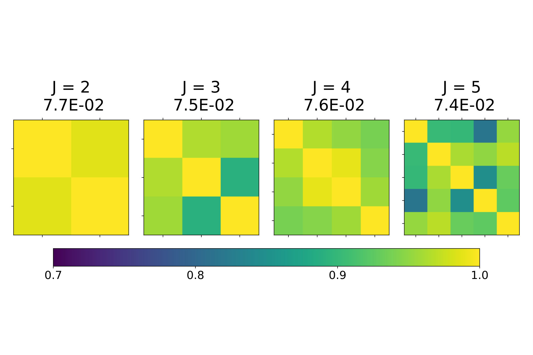 Figure 1
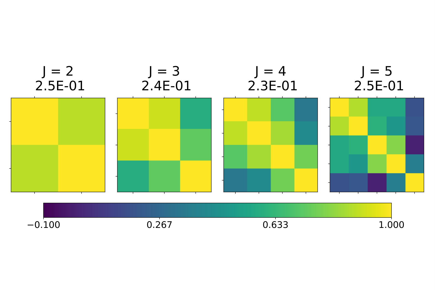 Figure 2
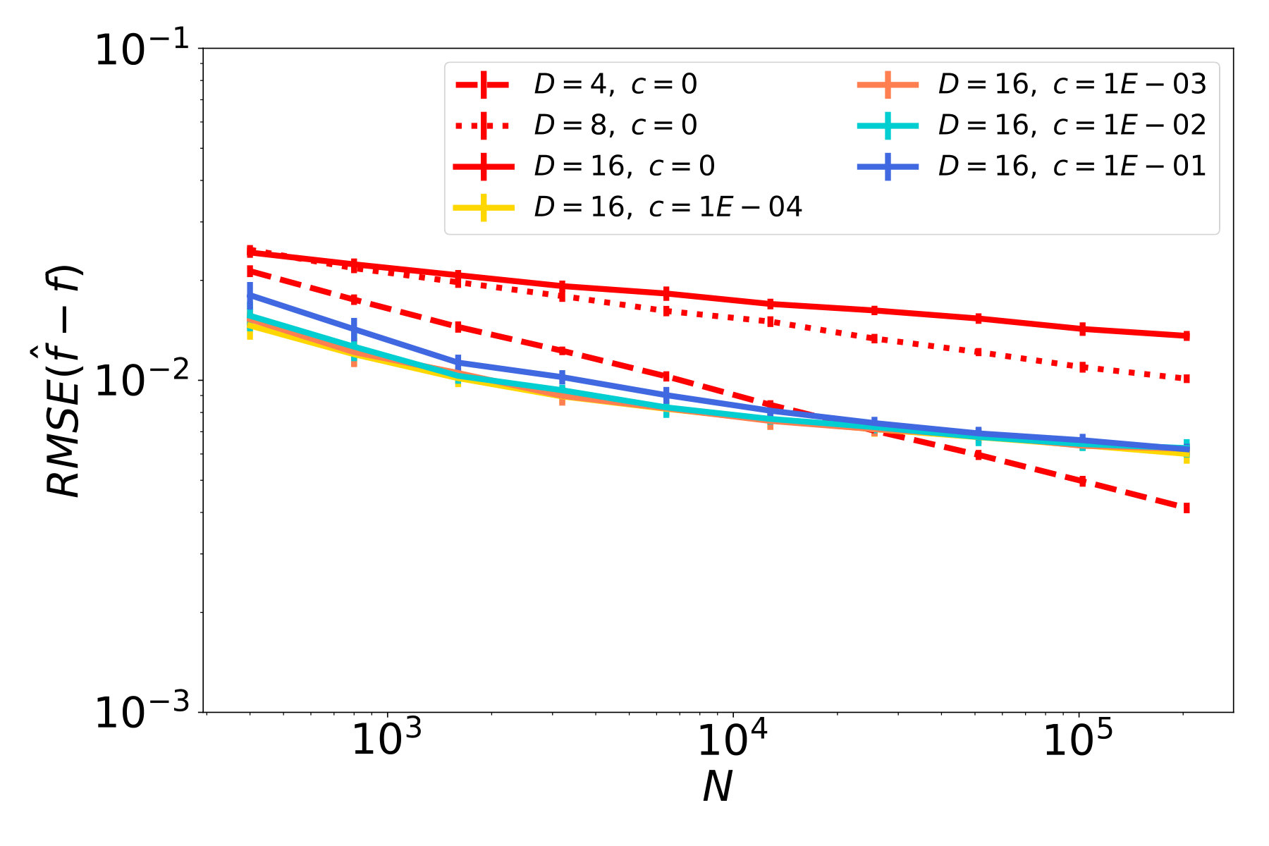 Figure 3
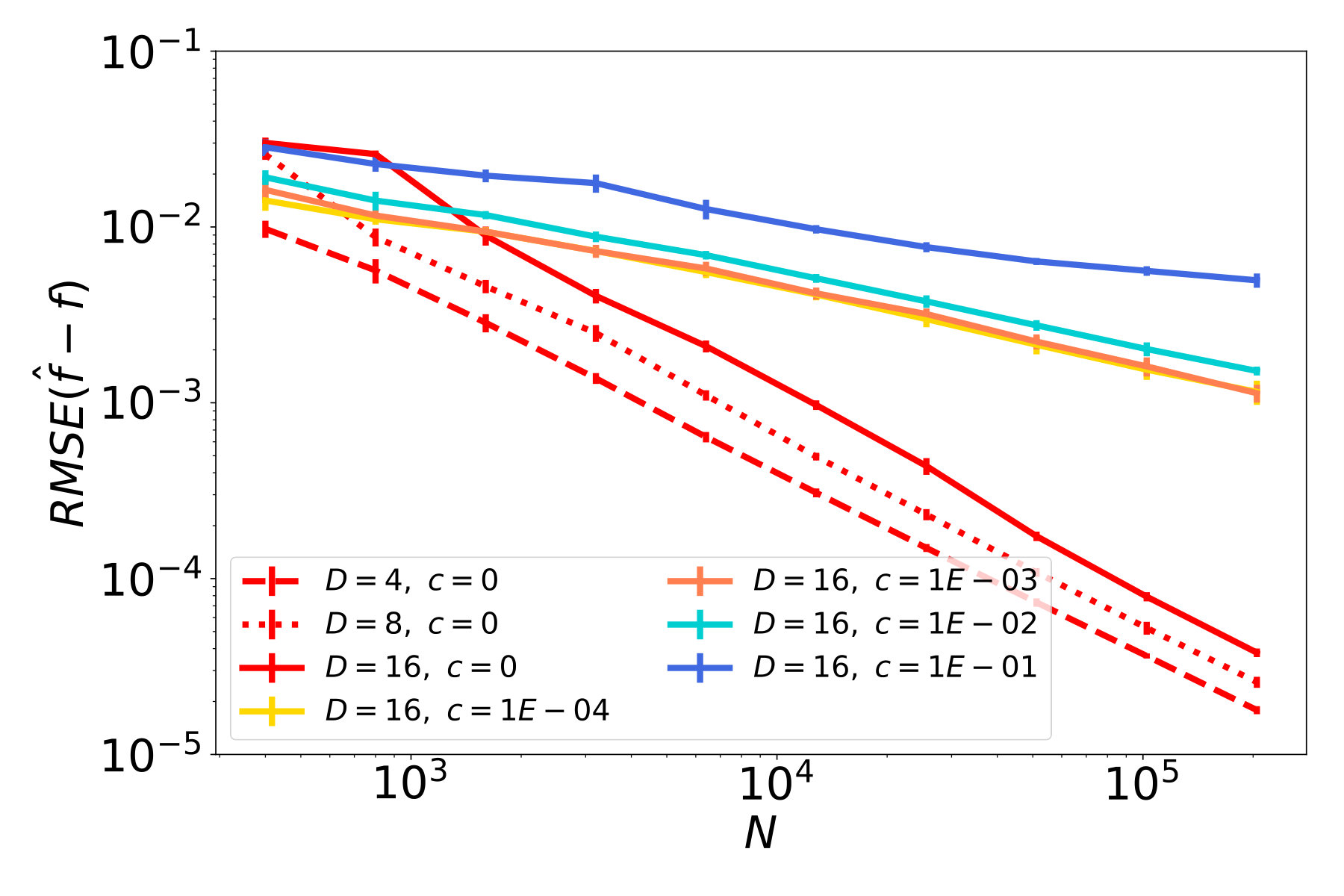 Figure 4
 Figure 5
 Figure 6
 Figure 7
 Figure 8
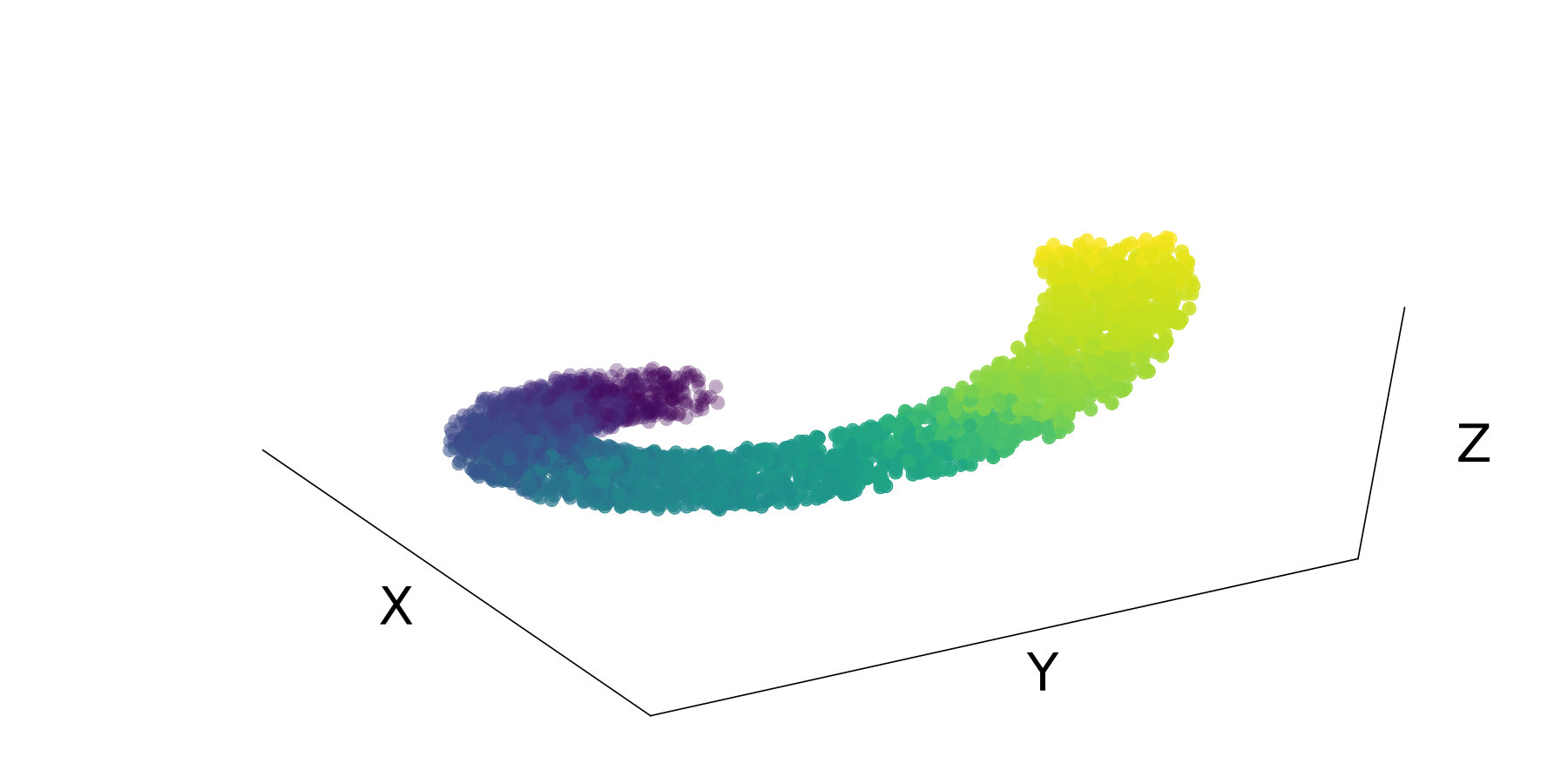 Figure 9
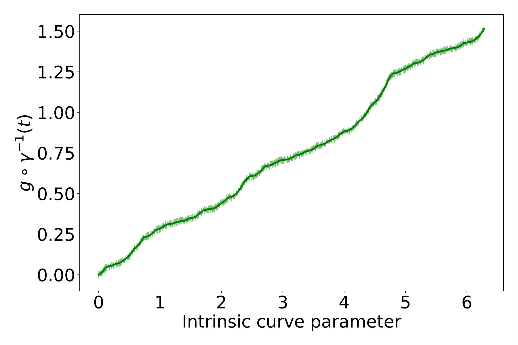 Figure 10
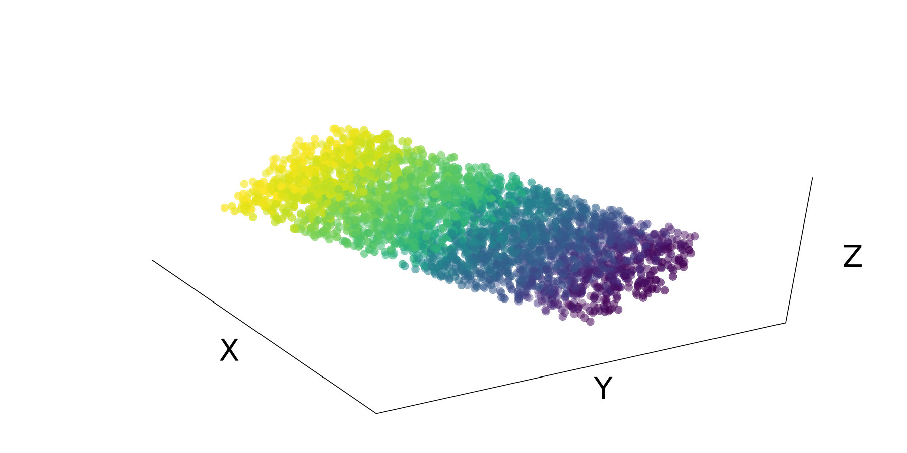 Figure 11
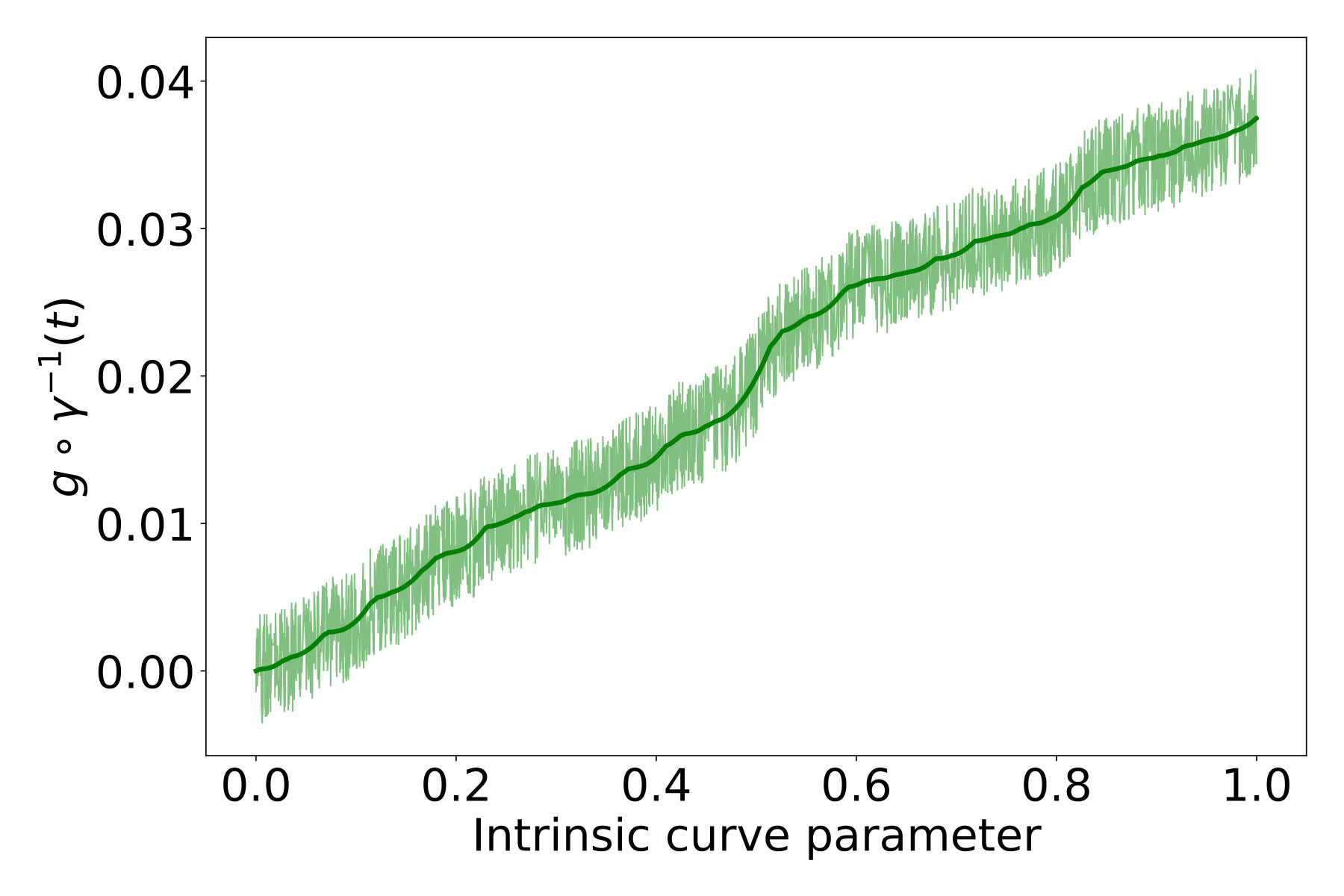 Figure 12
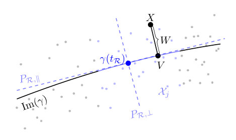 Figure 13
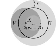 Figure 14
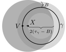 Figure 15
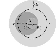 Figure 16
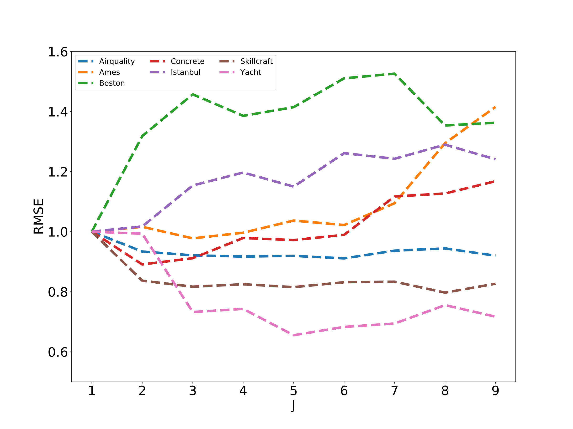 Figure 17
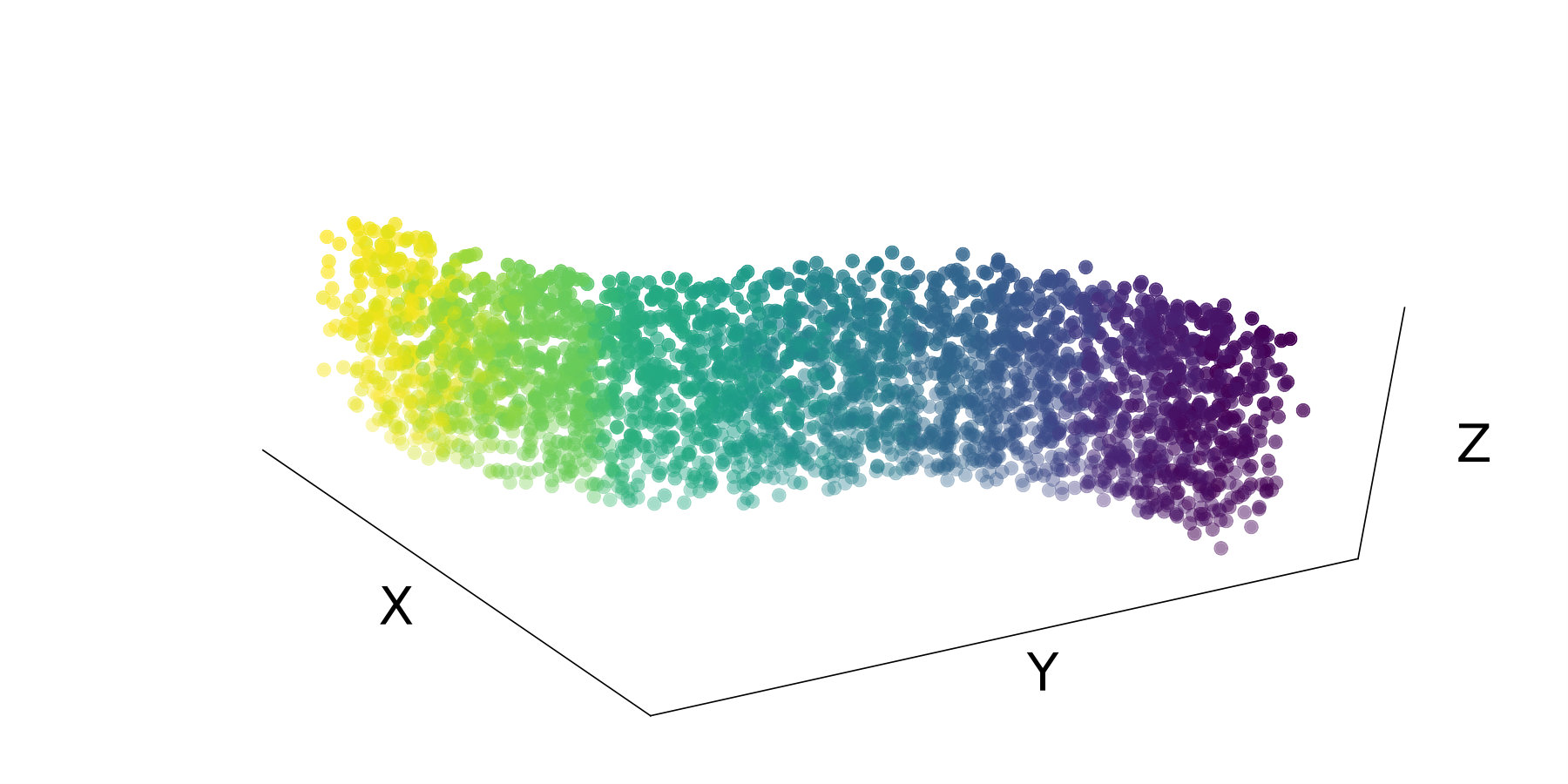 Figure 18
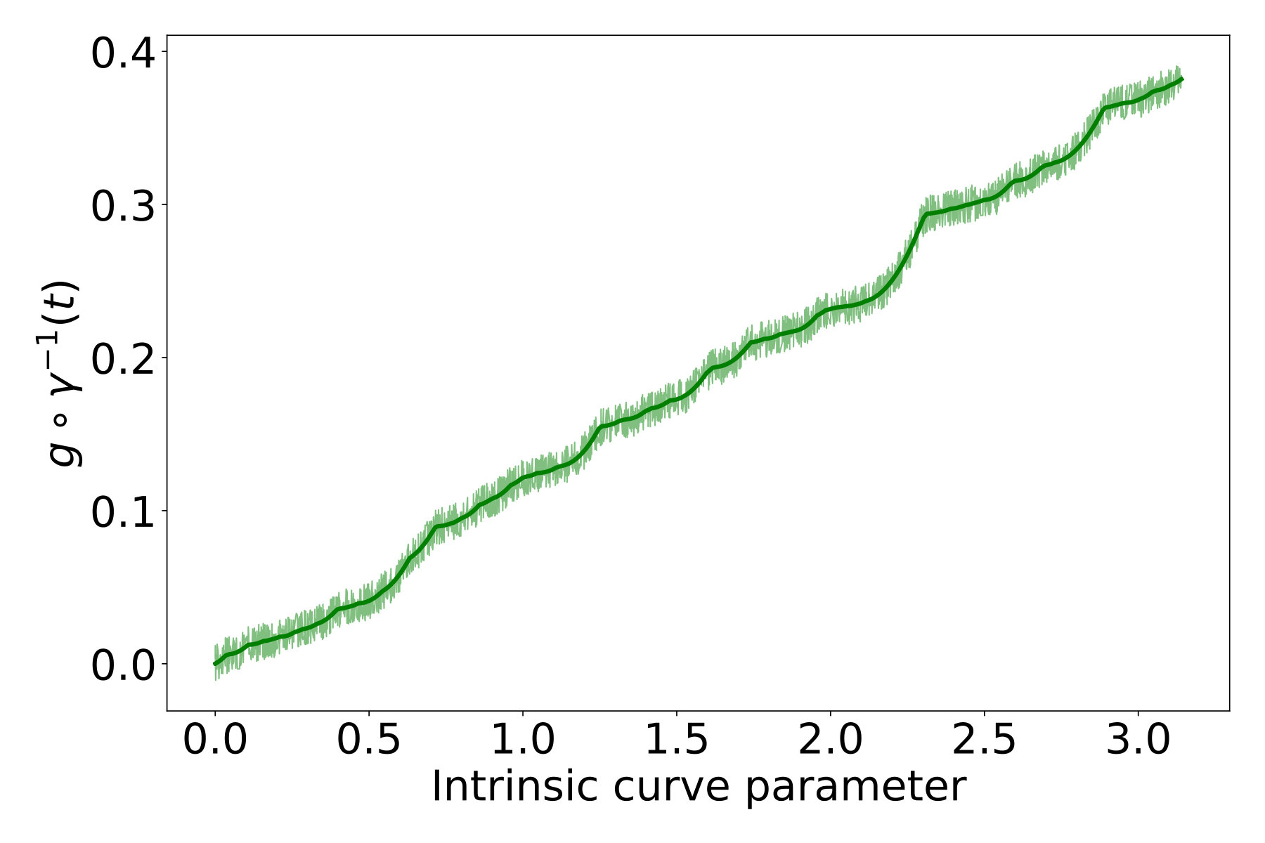 Figure 19
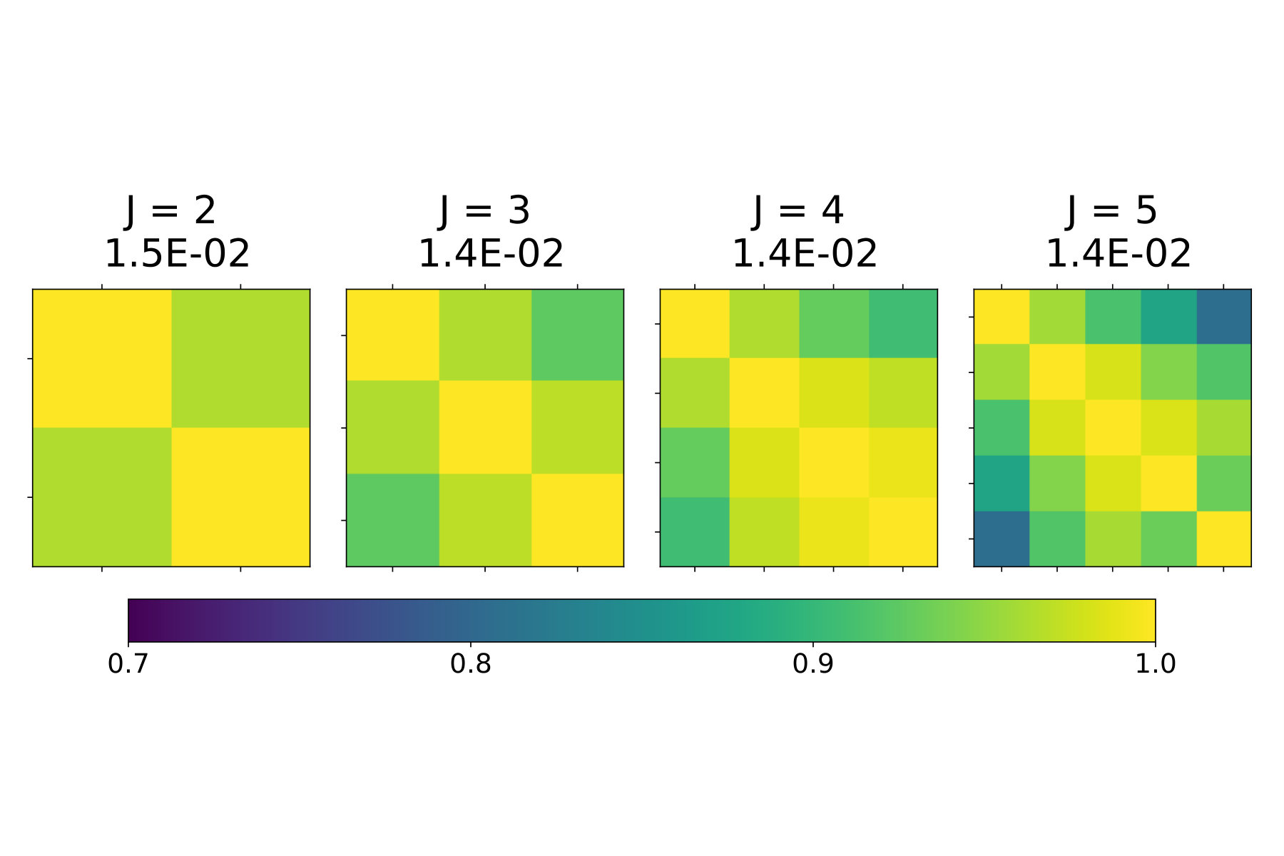 Figure 20
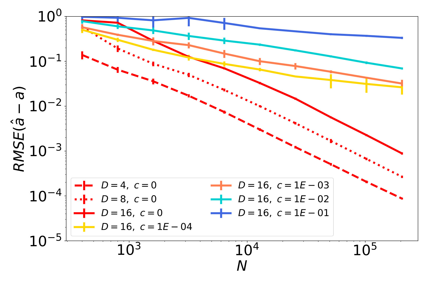 Figure 21
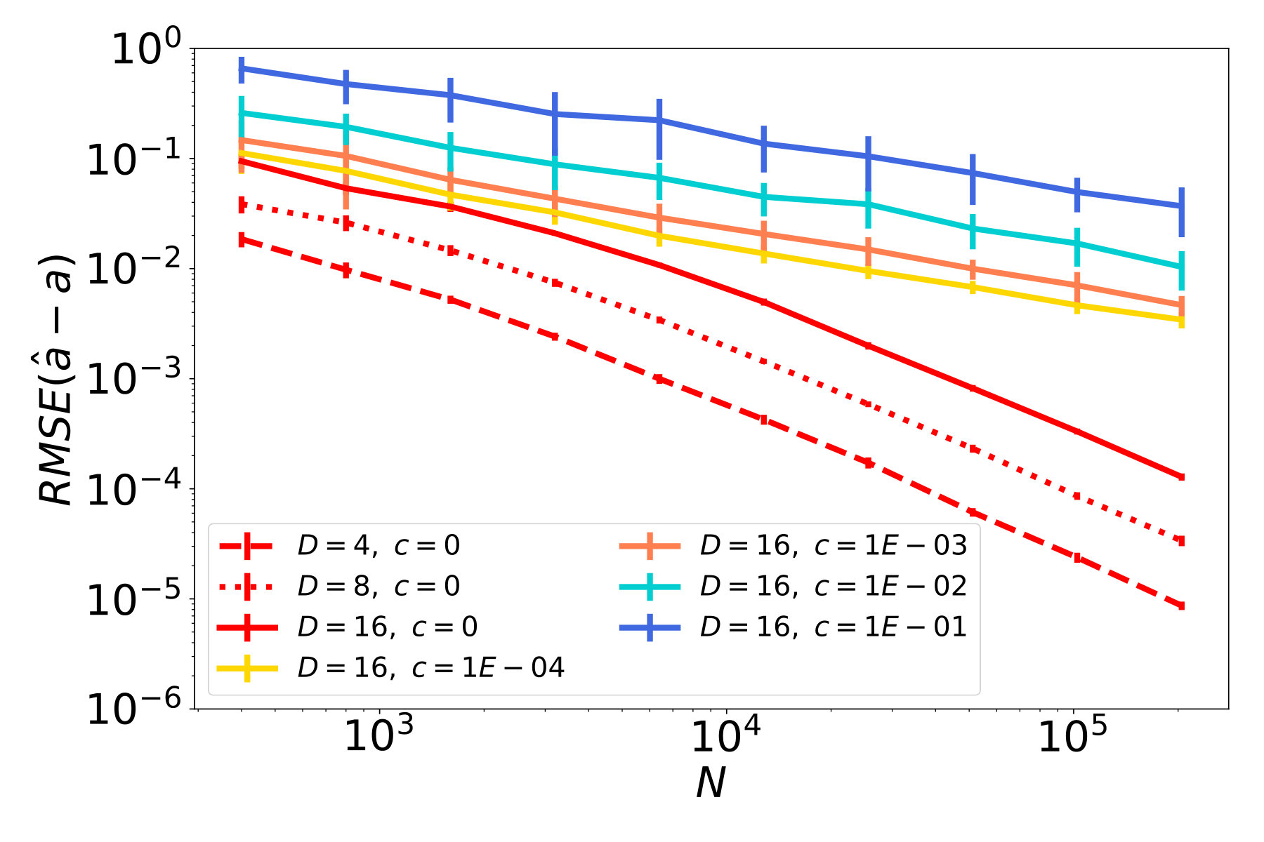 Figure 22
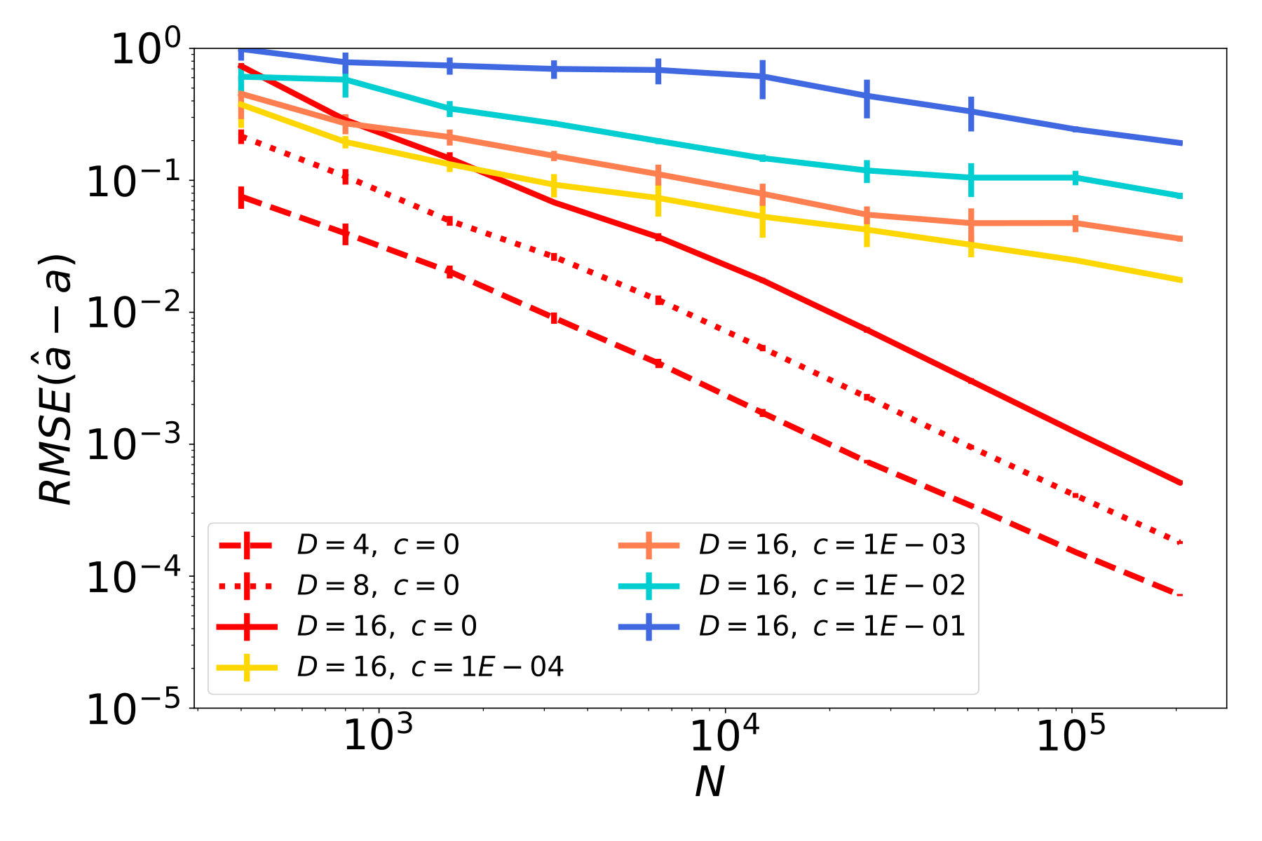 Figure 23
| symbol | definition |
|---|---|
| geometry | |
| is the parametrization of | |
| the orthogonal projection onto , see (3) | |
| geodesic distance for , extended by | |
| ball of radius around a point , with respect to a metric | |
| bound for the curvature of , i.e. | |
| \hdashline | projections onto the tangent/normal space at |
| here and | |
| probability | |
| random vector in with a distribution , and the marginal of is | |
| random vectors such that , where | |
| the expectation and the covariance of a random variable | |
| empirical mean and sample covariance over all samples | |
| shorthand for conditional mean and conditional covariance | |
| mean, and covariance, over samples that belong to ; | |
| constants | |
| the bi-Lipschitz constant of the function , see (10) | |
| number of level sets, i.e. the size of the partitioning of the data; , see (12) | |
| bound on the noise term , i.e., , where , see (A1) | |
| constant in bounding influence of cross-covariance, see (A3) | |
| lower-bound for non-zero eigenvalues in directions normal to , see (A4) | |
| bound for , see (A5) | |
| uniformity constant for the distribution along , see (A6) |
| NSIM | implication on SIM | comparable assumption in the literature |
|---|---|---|
| (A1) | the setting is often studied in SIM literature, e.g. in [16, 38] | |
| (A2) | for | integral part for inverse regression based techniques, usually implied by ellipticity, e.g. [29, 33, 34] |
| (A3) | implied by (A1) and (A2) | - |
| (A4) | for all , | implied by the constant conditional covariance assumption used sometimes for sufficient dimension reduction, e.g. [8, 27, 28] |
| (A5) | there exists such that | existing methods require to prove regression rates that do not depend exponentially on , e.g. [3, 22] |
| (A6) | is absolutely continuous with respect to the Lebesgue measure on the image of | this is common to ensure that the manifold is covered well enough, e.g. [32] |
| Characteristics | Yacht | Istanbul | Ames | Concrete | Air Quality | Boston | Skillcraft |
|---|---|---|---|---|---|---|---|
| -TF | Yes | No | Yes | No | No | Yes | Yes |
| Factor | |||||||
| Method | |||||||
| NSIM-dyad | |||||||
| NSIM-stat | |||||||
| Lin-Reg | |||||||
| kNN | |||||||
| SIR-kNN | |||||||
| Isotron | |||||||
| Iterations | |||||||
| ELM-Sig | |||||||
| Nodes | |||||||
| SNN-Tan | |||||||
| Nodes | |||||||
| SNN-Sig | |||||||
| Nodes |
| Term | Bound multiplied with | Shorthand notation |
|---|---|---|
Peer Reviews
No public reviews on file for this paper yet. If you reviewed it on a platform where reviews are public (OpenReview, ICLR, NeurIPS, ICML), you can paste yours below so the community can read it here.
Code & Models
Videos
No videos yet. Explain this paper in a talk, walkthrough, or lecture? Add one.
Taxonomy
MethodsLinear Regression
**
**Nonlinear generalization of the monotone single index model
Željko Kereta Email: [email protected] Simula Research Laboratory, Machine Intelligence Department, Oslo, Norway
Timo Klock Email: [email protected] Simula Research Laboratory, Machine Intelligence Department, Oslo, Norway
Valeriya Naumova Email: [email protected] SimulaMet, Machine Intelligence Department, Oslo, Norway
Abstract
Single index model is a powerful yet simple model, widely used in statistics, machine learning, and other scientific fields. It models the regression function as , where is an unknown index vector and are the features. This paper deals with a nonlinear generalization of this framework to allow for a regressor that uses multiple index vectors, adapting to local changes in the responses. To do so we exploit the conditional distribution over function-driven partitions, and use linear regression to locally estimate the index vectors. We then regress by applying a kNN type estimator that uses a localized proxy of the geodesic metric. We present theoretical guarantees for estimation of local index vectors and out-of-sample prediction, and demonstrate the performance of our method with experiments on synthetic and real-world data sets, comparing it with state-of-the-art methods.
Keywords: high-dimensional regression, dimension reduction, single index model, nonparametric regression, nonlinear methods
1 Introduction
Many problems in data analysis can be formulated as learning a function from a given data set in a high-dimensional space. Due to the curse of dimensionality, accurate regression on high-dimensional functions typically requires a number of samples that scales exponentially with the ambient dimension [41]. A common approach to mitigating these effects is to impose structural assumptions on the data. Indeed, a number of recent advances in data analysis and numerical simulation are based on the observation that high-dimensional, real-world data is inherently structured, and that the relationship between the features and the responses is of a lower dimensional nature [1].
The most direct such model, which has become an important prior for many statistical and machine learning paradigms, considers a -dimensional relationship of the form
[TABLE]
where is a random noise term, and the features and responses are related through an unknown index vector and an unknown monotonic function . Model (1) is called the single index model (SIM), and it first appeared in economical and statistical communities in the early 90s [15, 18]. Moreover, SIM provides a basis for more complex models such as multi-index models [5, 28, 42] and neural networks [24].
An assumption shared by SIM and generalizations is that there is a single lower dimensional linear space that accounts for the complexity in relating and . While simple, this assumption is only a first level approximation and is rarely observed in real-world regression problems. The goal of this paper is to relax the assumption on global linearity in the model (1), in order to locally adapt to changes in the relationship between and . Specifically, we propose the nonlinear single index model (NSIM), defined by
[TABLE]
where is a random noise term, is a bi-Lipschitz function, is a parametrization of a curve , and is the corresponding orthogonal projection, defined by
[TABLE]
Function can be seen as a univariate scalar function, defined on the parametrization domain , provided is a simple curve. This identification is useful for defining examples of the setting, and reveals SIM as a special example of (2), where .
Before formally describing the assumptions and details of our approach, let us begin with a couple of comments. Recall that smooth curves can be locally approximated by affine approximations, i.e., where is a local tangent vector of . Problem (2) can therefore be approximated by a family of problems of the type , where corresponds to pieces of that are approximately affine. Notice now that due to the monotonicity of , the proximity of and implies the proximity of and , and vice versa. Therefore, instead of looking at approximately affine pieces of , we can equivalently consider a partition of , consisting of disjoint intervals , and split (2) into a family of localized SIM problems
[TABLE]
where tangent vectors now play the role of index vectors in (1).
In Figure 1 we study the effects of such an approach on several UCI data sets111https://archive.ics.uci.edu/ml/datasets.html. Namely, for each data set we partition the data into sets, as detailed above, learn a SIM estimator on each of the sets, and then plot the generalization error of the resulting estimator as a function of the hyperparameter . Given sufficient amount of data, we can observe that replacing (1) with (4), its localized counterpart, often returns better estimation results. For example, on the Yacht data set the generalization error improves by more than percent for compared to SIM. Notice though that increasing the number of localized pieces does not always improve the performance. This can mostly be attributed to the fact that splitting the original data set into disjoint subgroups reduces the number of samples within each group, which has a detrimental effect on the variance of the estimator. In other words, we face a typical bias-variance trade-off, implying that hyperparameter needs to be carefully selected. Furthermore, sometimes a SIM is indeed the best fit to the data (e.g. Boston data set). As shown in the experiments in Section 5, this will be detected by our approach when combined with cross-validation to choose .
Related work.
To the best of our knowledge, relaxations of SIM have not yet been considered in this form. However, three research areas are highly relevant: linear single- and multi-index models, nonlinear sufficient dimension reduction, and manifold regression. Below we provide a short overview of the most significant and relevant achievements in each of these fields.
Single- and multi index models have been extensively researched, and we therefore, restrict ourselves to conceptually related work. Most studies focus only on the estimation of index vector(s), which started with the early work on linear regression based methods [4, 14, 31, 40]. The most relevant work is [16], where the authors use iterative local linear regression to estimate the index vector . Locality is enforced by kernel weights, which are initially set to be spherical around the estimation point, and then iteratively reshaped so that the isolines resemble level set boundaries of a strictly monotonous link function . This approach has been extended to the case of multiple index vectors [7], estimating instead the corresponding index space.
Another relevant line of work are methods based on inverse regression that began with the introduction of sliced inverse regression (SIR) [29]. This was followed by SAVE [8], PHD [30] , MAVE [46], Contour regression [28], Directional regression [27], etc. The common thread shared by these methods is the use of inverse moments, such as and , to estimate the index vector or the index space.
Several methods simultaneously learn the link function and the index vector. We mention Isotron [20] and Slisotron [19], which iteratively update the link function and the index vector; [10] that additionally assumes sparsity of the index vector; [6, 23] that use an iterative procedure and spline estimates; [38] that uses higher dimensional splines.
On the other hand, methods and theory for nonlinear sufficient dimension reduction are still in the early stages and there are many open questions. Most of the existing studies consider kernelized versions of linear estimators (such as SIR or SAVE) to globally linearize the problem in feature space, and then apply well-known regression methods, see [25, 26, 45, 47].
Model (2) can also be considered from the viewpoint of manifold regression, where the goal is to estimate a function defined on the data. Manifold regression methods, such as [3, 22, 36], generally assume that the marginal distribution of is either supported on or in its close vicinity. As a consequence, Euclidean distances can be used to locally approximate the geodesic metric. This is a strong assumption which is implicitly or explicitly leveraged by all manifold regression techniques, and presents a breaking point for their effective use. In this work, we instead consider distributions that are spread in all directions of the ambient space around the curve . Consequently, geodesic proximity cannot be inferred from Euclidean distances and we instead need to locally approximate the geodesic distance.
Main idea and estimation procedure for the NSIM model.
Model (2) increases the flexibility of the ordinary SIM by allowing for varying index vectors, corresponding to different regimes of the response . Consequently, a natural approach would be to partition the data into several groups, based on , and use a SIM-like estimator to approximate the index vector and the regression function. In particular, our approach follows three steps.
In the first step we partition the data set into sets, and . To do so we define a disjoint union of the responses, for intervals , and then set
[TABLE]
We refer to sets as level sets, since they can be defined as in the noise-free case. The optimal method for partitioning as depends on the marginal distribution of , and is best chosen after inspecting the empirical density. For example, we suggest using dyadic cells of if the density of is roughly uniform, and stochastically equivalent blocks if the probability mass is unevenly distributed.
In the second step we compute estimates of local index vectors by using linear regression on and . Namely, let be the standard finite sample estimate for the conditional covariance , where denotes the empirical expectation. Then, set , where is the solution of linear regression,
[TABLE]
or equivalently,
[TABLE]
Intuitively, vectors correspond to directions in which the function changes, and therefore approximates local gradient directions of . In the case of an ordinary SIM, it has been shown in [2] that the direction of the global linear regression vector, denoted by , is an unbiased estimator of index vector , if has elliptical distribution. Furthermore, is asymptotically normal, hence achieves -consistency. As we will see in Sections 2 and 3, in our case the analysis of is more challenging due to the underlying nonlinear geometry.
In the final step we use a kNN-type estimator to predict for an out-of-sample . Since the make-or-break point of kNN-estimators regards how are distances between and training samples measured, the critical point of this step is about the selection of an appropriate distance function. The issue is that the optimal choice (the geodesic metric on ) is not available since is not known, and the naive choice (the Euclidean metric) generally leads to estimation rates that depend on the ambient dimension, and thus the curse of dimensionality.
To develop a proxy metric, consider now the ordinary SIM. Here the geodesic metric is equivalent to the Euclidean distance of projected samples if approximates the true index vector with a sufficiently high rate, i.e., is a good proxy for the geodesic metric provided is small. Moreover, training the kNN estimator on projected samples achieves optimal univariate regression rates. The NSIM case is more challenging because first, we have different index vectors to choose from, and second, cannot be a priori assigned to any level set since is unknown. Still, if we assign to each sample the index vector , where is the unique level set with , we can show that
[TABLE]
approximates the geodesic metric reasonably well, under suitable choice of the restricting radius , see Section 4.2. In the special case of a perturbed SIM, where is not too far from an affine space, this is also true for , see Section 4.1.
This motivates the following estimator: let denote the -th closest sample to when measured in , and where ties can be broken arbitrarily. Then set
[TABLE]
As we will discuss in Section 4.2, the radius plays a dual role. It needs to be large enough so that there are enough samples to choose neighbors from, but small enough so that (8) is a good proxy for the geodesic metric. The entire estimation approach is summarized in Algorithm 1.
Computational complexity.
The first two steps, partitioning and computing tangents, are dominated by , which is mostly due to forming covariance matrices and computing the generalized inverse. Out-of-sample prediction requires operations per evaluation.
Contributions and organization of the paper.
In this work we introduce a nonlinear generalization of the SIM and study estimation of the model from given data points sampled iid. from an unknown distribution . The presented model synthesizes the fields of linear sufficient dimension reduction and manifold regression, thereby attempting to extend both. We first develop a rigorous mathematical framework, in Section 2, through which NSIM can be theoretically analyzed.
We provide a simple and efficient estimator based on output-conditional linear regression and kNN-regression. Theoretical guarantees of the approach are subjects of Sections 3 (local index vectors) and 4 (function estimation). In summary, we achieve optimal estimation rates [13, 21] in the noise-free scenario ( almost surely), or if the data follows the ordinary SIM. In the general case, the estimator remains biased.
The theoretical analysis on local index vector (or tangent field) estimation requires a careful study of (conditional) ordinary linear regression (6). In particular, two sources of error are present: a bias term, that decays when increasing the number of subsets in the level set partition, and a variance term, that decays with the number of samples . Our analysis reveals a concentration bound of the form
[TABLE]
where is a curvature bound for . This is a surprising result because both the bias and the variance decrease with (as long as the noise is negligible compared to the ). This observation is a key component for establishing optimal regression rates in the noise-free case.
For the regression analysis, we show in Section 4 that is equivalent to the geodesic metric , up to an error made in tangent field estimation. This suffices to establish aforementioned kNN-regression guarantees. These results are relevant from a more general perspective, because they can readily be used with other means of estimating the tangent field, and can be extended to higher dimensional manifolds.
In Section 5 we conclude the paper with extensive numerical tests on synthetic and real data sets, that have previously been used as benchmarks for the SIM model. The results show that the extended flexibility of NSIM is beneficial for both, out-of-sample prediction and model interpretability.
General notation.
We use for . denotes the Euclidean norm for vectors, and the spectral norm for matrices. denotes the geodesic metric on . Provided that is an arc-length parametrization, this means . We extend the notation to by setting whenever projections are uniquely defined. For a discrete set of points we use to denote its number of elements. On the other hand, if is a connected subsegment of or if is an interval, then denotes its length. By an interval we always refer to a closed and connected subset of the real line. We use and . The Moore-Penrose inverse of a matrix is denoted by .
The abbreviation a.s. is used as a shorthand for almost sure events (with respect to implicit random vectors), and iid. refers to independent and identically distributed data sampling. Table 1 contains an overview of notation and constants used in this paper.
2 Theoretical framework for the NSIM model
Due to the broadness of its scope, it is relatively easy to construct examples of NSIM that fit the model but for which estimation from finite samples is not possible. The goal in this section is to define a framework that allows a rigorous analysis, yet is broad enough to encompass both the SIM and its nonlinear generalization NSIM. In the following we describe the assumptions on the function class, the underlying nonlinearity , and on the distribution of the data set.
Regularity assumptions for and .
Let , for an interval , be an arc-length parametrization of a simple, connected, and smooth curve, denoted , and set . We consider Lipschitz functions that satisfy for some -bi-Lipschitz function , that is
[TABLE]
Through rescaling we can always assume . We can, without loss of generality, align with , i.e., choose an orientation such that , for almost every . An important quantity is the reach of - the largest such that any point at distance less than from has a unique nearest point on [9]. This ensures that , and thus , is well defined for all within the reach, i.e., all such that .
Distributional assumptions.
We consider distributions for which the distribution of is absolutely continuous with respect to the Lebesgue measure on for any non-empty interval , and which satisfy assumptions (A1) - (A6) below.
Assumptions (A1) - (A4) are related to single- and multi-index model literature (or more broadly sufficient dimension reduction literature, see [34] for a review), whereas (A5) - (A6) are related to manifold regression. We begin by describing the behavior of the noise .
- (A1)
For , we assume \varepsilon\mathchoice{\mathrel{\hbox to0.0pt{\displaystyle\perp\hss}\mkern 2.0mu{\displaystyle\perp}}}{\mathrel{\hbox to0.0pt{\textstyle\perp\hss}\mkern 2.0mu{\textstyle\perp}}}{\mathrel{\hbox to0.0pt{\scriptstyle\perp\hss}\mkern 2.0mu{\scriptstyle\perp}}}{\mathrel{\hbox to0.0pt{\scriptscriptstyle\perp\hss}\mkern 2.0mu{\scriptscriptstyle\perp}}}X|\pi_{\gamma}(X), and a.s..
In sufficient dimension reduction problems, \varepsilon\mathchoice{\mathrel{\hbox to0.0pt{\displaystyle\perp\hss}\mkern 2.0mu{\displaystyle\perp}}}{\mathrel{\hbox to0.0pt{\textstyle\perp\hss}\mkern 2.0mu{\textstyle\perp}}}{\mathrel{\hbox to0.0pt{\scriptstyle\perp\hss}\mkern 2.0mu{\scriptstyle\perp}}}{\mathrel{\hbox to0.0pt{\scriptscriptstyle\perp\hss}\mkern 2.0mu{\scriptscriptstyle\perp}}}X|\pi_{\gamma}(X) is often more commonly written Y\mathchoice{\mathrel{\hbox to0.0pt{\displaystyle\perp\hss}\mkern 2.0mu{\displaystyle\perp}}}{\mathrel{\hbox to0.0pt{\textstyle\perp\hss}\mkern 2.0mu{\textstyle\perp}}}{\mathrel{\hbox to0.0pt{\scriptstyle\perp\hss}\mkern 2.0mu{\scriptstyle\perp}}}{\mathrel{\hbox to0.0pt{\scriptscriptstyle\perp\hss}\mkern 2.0mu{\scriptscriptstyle\perp}}}X|\pi_{\gamma}(X).
The next assumption states that is centered in the middle of the distribution.
- (A2)
holds -a.s.
This is inspired by the linear condition mean assumption from single- and multi-index model literature, and is an integral component of every method based on inverse regression [33, 34]. It is needed to ensure the recovery of a subspace of the index space in the population regime , see e.g. [8, 29], and is often ensured by a stronger condition: if is elliptically distributed [33]. (A2) also implies identifiability of by the distribution of .
Lemma 1**.**
Let , with orthogonal projections defined according to (3), and let be a random vector such that and are a.s. unique. Let and be measurable and injective. If , and a.s., then a.s..
Proof.
Due to the assumption we have
[TABLE]
Since conditioning on an injective function of a random variable is equivalent with conditioning on the random variable itself, we get
[TABLE]
and similarly for . Plugging into (11) the claim follows. ∎
In the linear case (A1) and (A2) imply for any interval , where is the orthoprojector onto the index space, and . For some single- or multi-index model estimators this suffices to ensure the recovery of the index space in the population regime, see e.g. [29]. In the nonlinear case however, due to curvature we require an additional assumption. Let be the induced random variable and define the mean , the tangential projection , and the orthogonal projection , see Figure 2. Furthermore, let be the shortest connected segment with .
- (A3)
There exists an absolute constant such that
Due to other assumptions, (A3) trivially holds if is replaced by , though we need more regularity. Namely, our analysis shows that replacing with , for some , approximations of the tangent field are valid only if falls below a certain threshold. Thus, for this restricts the analysis to only SIMs and curves with small curvature. We select for the sake of notational simplicity, though the results are valid for any .
Our fourth assumption describes the behavior of orthogonal to the curve.
- (A4)
For all , with , we have
[TABLE]
In the nonlinear case an assumption of this form is necessary in order to ensure that the solution of local linear regression aligns with the local tangent vector instead of the local curvature vector. This is also observed numerically, where if the variance vanishes, as a function of , a vector close to a local curvature vector can minimize (6). Such an assumption has also been used for multi index models, see [8, 27, 28], though assuming (A1) and (A2) would suffice in our case to ensure that the linear regression vector (for any conditioning on ) is contained in the index space.
The last two assumptions deal with properties of the distribution along the curve , denoted by , and with components orthogonal to it, denoted by .
- (A5)
, the component of orthogonal to , satisfies , -a.s.
An assumption of this type is needed due to the fact that the projection , and consequently the function , is not always well defined for . In case of a straight line we have , and thus there are no restrictions on (which reflects standard SIM assumptions). On the other hand, (A5) is a relaxation of standard assumptions in manifold regression, which require samples to lie on, or very near the manifold, i.e., or .
Lastly, we assume that the data distribution along the curve does not deviate too much from a uniform distribution. This is used in manifold regression approaches that approximate the manifold by localization and linearization, as it ensures that local pieces are sufficiently well covered, see e.g. [32].
- (A6)
For random vectors there exists such that holds for any .
A comparison of assumptions (A1)-(A6) with standard assumptions in the literature, and their implication in case of the SIM, is provided in Table 2.
3 Learning localized index vectors
We now begin with the analysis of our estimator by providing guarantees for the estimation of local index vectors in terms of , the number of samples, and , the number of level sets. The estimation of local index vectors follows three steps:
- Step 1
Partition ’s according to a dyadic partitioning of the range222Technically, we ought to use , and to account for noise at the boundaries, but for the sake of simplicity we assume is thresholded to , such that for all . ,
[TABLE] 2. Step 2
Estimate local index vectors with , where is the solution of (local) linear regression for samples ,
[TABLE] 3. Step 3
Assign index vectors to samples by setting .
Denote now the tangent vectors by and , where . Because of the quantization in Step 3, index vector estimation error can be decomposed as
[TABLE]
where is the infimum of all connected pieces of such that , and its curvature bound. Since as long as (by Lemma 11), the second term can be improved by increasing the number of level sets . On the other hand, for the first term we can prove the following concentration bound.
Theorem 2**.**
Let , , and . Define . Provided Assumptions (A1) - (A5) hold, there exist constants , depending polynomially on , , , , , , , such that whenever
[TABLE]
we have
[TABLE]
The first condition in (15) deals with linearization, and effectively bounds the influence of the cross-covariance term from (A3). The condition gets easier to satisfy for shorter , or shorter . This goes in line with the discussion in Section 2, since by isolating shorter segments of , NSIM approaches the SIM, where the condition in (15), and assumption (A4), are trivally satisfied. For a weaker form of (A3), namely , we obtain the same result with replacing , and replacing , see Theorem 16.
The second condition in (15) implies that, locally, there is a minimal number of samples needed to ensure that the norm of the linear regression solution is bounded from below.
Lastly, we note that are proportional to powers of , which implies that they are uniformly upper bounded (independent of ) if is uniformly bounded from below. We show in Lemma 14 in the Appendix that this is indeed the case whenever and is bounded from below. The latter is satisfied if for example , see Lemma 14. Due to the bi-Lipschitz property of , it seems reasonable however that is bounded from below in more general scenarios. The requirement , on the other hand, is also observed numerically, precisely because vanishes as soon as is small. This suggests that our analysis correctly identifies the dependency on .
Remark 3** (Special cases of Theorem 2).**
- :
In the noise-free case the lower bound for is removed. Thus, provided is kept constant and , we achieve . This proves a rate for the estimation of the (local) index vector with the ordinary least squares estimator for strictly monotonic link functions. 2. :
If corresponds to a flat piece of the curve the first term in (16) vanishes. Thus, is an unbiased estimator of , with convergence rate , provided is kept constant and . This result covers the SIM, and our estimation rate matches other results [2, 4, 16].
Recalling decomposition (14), Theorem 2 can now be used to bound for all by invoking a union bound argument over all level sets , .
Corollary 4**.**
Let Assumptions (A1) - (A6) hold. Let and assume we have iid. copies of . Assume we partition the data set into partitions according to (12), so that
[TABLE]
and , and compute local index vectors . There exist constants , depending polynomially on , , , , , , , such that if
[TABLE]
we have
[TABLE]
Let us make two remarks. First, terms in the bound on the right hand side of (19) can also be written in a local form, i.e., a global curvature bound can be replaced with a curvature bound for a segment around the sample . Thus, the learning of local index index vectors is consistent on locally linear pieces.
Second, (17) and (18) suggest that to optimally balance bias and variance we ought to use level sets, where is small enough so that (18) is satisfied. Looking at (19), this implies that there are two regimes.
In the first regime, in order to decrease the error we ought to increase as long as , i.e., subdivide the data set into an increasing number of subsets, while keeping the number of samples within each subset roughly constant. The rationale behind this is that further subdividing the data set not only reduces the approximation error (which is caused by the curvature), but it also reduces the variance in the linear regression part of the problem, i.e., when estimating by . In the second regime function noise precludes further decreasing , since we cannot further decrease . In other words, the noise level imposes a lower bound on , and the bias does not completely vanish.
Note also that in (19), compared to (16), we lose an order in , i.e., in the interval length. This is due to the use of quantization to approximate the entire tangent field over the respective level set. This could be improved by learning a separate tangent for each sample from a level set centred around , but the second term in (19) prohibits achieving overall.
4 Function estimation
In this section we use the guarantees on local index vector estimation to establish function estimation guarantees. We recall that the estimator (9) predicts an output by averaging the responses of , the closest samples with respect to the metric . This makes the analysis challenging because the same data is used twice: first for estimating the geometry and then for predicting the function. As a result, random variables become statistically dependent and their finite sample average could be biased.
To avoid this technical issue split the given data set (consisting of samples) in two halves (reducing the effective sample size only by a factor of ) and use the first half, , for approximating the geometry, and the second half, , for function prediction. We then extend the tangent field approximation through nearest neighbors, defining , where . The prediction of is then given by averaging the responses, , of closest samples with respect to from , see Algorithm 2. Thus, random variables are not used in the selection of closest neighbors of and we preserve unbiased finite sample averages, i.e., .
We split our analysis in two parts. The first concerns the case when is close to an affine space (see Definition 5), and we call it a perturbed single index model. The second part extends the analysis to general curves . The reason for treating the first case separately is that we can achieve theoretical guarantees even without restricting the search space of nearest neighbors, i.e. setting . Furthermore, numerical experiments in Section 5 suggest that perturbed SIMs fit well to several data sets that were previously used as benchmarks for the SIM.
4.1 Function estimation for perturbed single index models
We begin by defining the notion of almost linearity that is used to quantify the deviation of the true model to an ordinary SIM, respectively, of the curve to a straight line.
Definition 5**.**
Let be an interval and an arc-length parametrized curve. Let . We say is -almost linear if for all .
Definition 5 implies that if is close to then is close to a straight line. Furthermore, the Euclidean distance approximates the geodesic distance well, i.e. for any , which allows to prove an equivalence between the (unrestricted) proxy metric and .
Proposition 6**.**
Assume is -almost linear for some . Let , and be arbitrary sets. Let . If is -th closest sample, based on , and the -closest sample, based on , we have
[TABLE]
Note that curvature and reach of a curve always satisfy . This means that is trivially satisfied, since by (A5). Thus, the requirement is driven by linearization, namely, by the fact that we are approximating the geodesic geometry of samples projected onto a curved space, with a linear geometry of samples projected onto its linerization.
To show guarantees for function estimation we first need to derive bounds on the tangent field from bounds on , given by Corollary 4. Using Proposition 6 with sets and , for all we have
[TABLE]
where is the sample closest to with respect to the geodesic distance. We can now state the main result for function estimation.
Theorem 7**.**
Assume (A1) - (A6). Let and assume that is -almost linear for some . Whenever satisfy the conditions of Corollary 4, we have for arbitrary and
[TABLE]
with probability at least , where are constants from Corollary 4, is an absolute constant and .
Proof.
We first decompose the left-hand side of (22) as
[TABLE]
The first term is a sum independent copies of . Since almost surely, and , Höffding’s inequality for bounded random variables gives, for an absolute constant
[TABLE]
Assume now and are -nets for with respect to . We can use the Lipschitz property of and apply Proposition 6 to bound the second term as
[TABLE]
Using (21) and we get
[TABLE]
Lemma 20 gives that and are -nets for with probability . The claim then follows by Corollary 4. ∎
Theorem 7 reveals that the error in function estimation originates from three sources. The first term accounts for the averaging of the noise, which is incurred by responses . Using , as is standard for Lipschitz-smooth functions, it decays at a rate . The second term bounds the geodesic distance to the nearest neighbor, and comes from the covering of the curve by the projected samples. The last two terms are from the approximation of the geodesic metric with the proxy metric through tangent approximations , and behave according to Corollary 4. Setting and , as in Section 3, yields
[TABLE]
We see that the estimator is generally biased since the error tends to for .
Remark 8** (Special cases of Theorem 7).**
- :
In the noise-free case the first term in (22) vanishes, and thus choosing , and with small enough so that (18) holds, we have
[TABLE]
Up to logarithmic factors, this matches the optimal rate for noise-free estimation of Lipschitz functions, see [21]. 2. :
If the model follows the ordinary SIM the second term in (23) vanishes. Thus we achieve a rate, which is optimal for Lipschitz smooth functions [13].
Before moving to general curves, let us remark why achieving consistent estimation is a challenging task in the noisy, nonlinear case. The presented estimator is based on localization and linearization, where localization hinges on the fact that conditional distributions are increasingly SIM-like when reducing the level set width . This reduces the effects of curvature and linearization becomes increasingly accurate. On the other hand, relating the width of with the length of corresponding segment of the curve, as , is by Lemma 11 valid only if . Namely, reducing beyond that threshold does not reduce , i.e., does not become more SIM-like. This predicament can not be further improved under our noise model.
Results in this section imply that having a consistent estimator of the tangent field of , whose sample complexity does not depend exponentially on , is sufficient to construct a consistent estimator for , with a similar sample complexity. At the same time, a consistent, low-complexity estimator of can be used to estimate the tangent field, by approximating through finite sample differences. This suggests a certain equivalence between estimating and estimating the tangent field of , and to some extent the manifold itself.
Minimax rates for estimating a manifold from samples that are spread around it have been extensively studied in [11, 12]. Moreover, in [12] the authors provide a theoretical estimator that converges at a rate (measured in the Hausdorff distance), where is the dimensionality of the manifold. However, they emphasize that the estimator is not practical and pose the development of a practical alternative as an important open problem. To the best of our knowledge, this problem still has not been solved.
4.2 Extension to general curves
In the general case the unrestricted proxy metric is not equivalent to the geodesic metric , and thus cannot be used to reliably select nearest neighbors. To better illustrate this point, let be a segment of the unit circle that contains two antipodal points and , and assume we have access to the true tangents , , so that . Thus, on one hand we have , and on the other since .
To avoid this and establish an equivalence between and , similar to Proposition 6, we thus have to restrict the search space. Considering the unit circle example, we ought to choose that ensures there are no two points , such that , but and . It can be shown that this is satisfied for , provided assumption (A5) holds, see Figure 3 and Lemma 22. On the other hand, needs to be large enough to ensure there are enough samples within , with respect to , to achieve optimal function prediction rates. Under the uniformity assumption (A6), this is ensured whenever .
Balancing these two demands we get and thus . Therefore, we require a more restrictive version of (A5). To compensate for errors in tangent approximations we further impose . This allows to prove a guarantee for metric equivalence.
Proposition 9**.**
Assume (A5) for for some , and choose any . Let , and be arbitrary sets. For an arbitrary let be its -th closest sample based on , and be its -closest sample based on . Whenever forms a -net on , and
[TABLE]
we have
[TABLE]
Covering the manifold with a sufficiently fine -net , and condition (25), are satisfied with high probability as soon as is sufficiently large, due to Corollary 4 and Lemma 20, respectively. In that case, Theorem 7 holds also for general curves, by simply replacing Proposition 6 with Proposition 9 in the proof. Since for the term converges to by Corollary 4, we are ensured to enter the valid regime whenever the noise is small enough compared to (in particular in the noise-free case).
Proposition 10**.**
Assume (A1) - (A6), and the conditions of Proposition 9 hold. Let . Whenever , satisfy the conditions of Corollary 4, we have for arbitrary and
[TABLE]
with probability at least , where are constants from Corollary 4, is an absolute constant and .
5 Numerical Experiments
In this section, we present experimental results of the proposed estimator in two settings. First, we conduct synthetic experiments to validate theoretical results of Sections 3 and 4. Second, we benchmark the estimator against commonly used methods on a selection of real-world data sets. The source code for Algorithm 1 and synthetic experiments is available at https://github.com/soply/nsim_algorithm. Moreover, real-world data sets, code for their preprocessing, and implementations of competing estimators (or references, if publicly available source code is used) are readily available at https://github.com/soply/local_sim_experiments.
5.1 Experiments with synthetic data
General setup.
We consider the following three curves
[TABLE]
and embed them into for . We set , where is sampled uniformly on , is sampled uniformly on , and the rows of form an orthonormal basis for the normal space of at . Examples of such marginal distributions are illustrated in the top row of Figure 4. The target function is a strictly monotonic, piecewise quadratic polynomial. We set with . Different noise levels are used: with and .
Parameter selection for the NSIM estimator is guided by Section 4. Namely, we use and if , and with cross-validation over in the noisy case. Furthermore, the restricting radius for the nearest neighbor search is . We also train an ordinary kNN-regressor with in the noise-free case, and in noisy case, to demonstrate that in these problems ordinary kNN-regression indeed suffers from the curse of dimensionality.
For evaluating the NSIM estimator, we report the root mean squared errors (RMSE)
[TABLE]
where are test samples iid. from , and is chosen as described above. The results are averaged over 20 repetitions of the same experiment. The standard deviation is indicated by vertical bars.
Discussion
The results of our studies are presented in Figure 5. In red plots, which correspond to cases with , we observe a decay of the function error (Figures 5a - 5c), and similarly a decay of the tangent field error (Figures 5d - 5f). In particular, the ambient dimension affects the error only in terms of a multiplicative constant but not in the rate of decay. Therefore, the NSIM estimator does not suffer from the curse of dimensionality, which is not the case for ordinary kNN-regression as shown in Figures 5g - 5i.
The remaining plots in Figure 5 represent noisy cases, where the highest noise level corresponds to blue lines. Considering the first column, where is a straight line, and therefore the data follows an ordinary SIM, we see that the error for function and index vector estimation steadily decreases at a rate. This confirms our theoretical result, i.e., the NSIM estimator is consistent, and achives the optimal rate, in case of an ordinary SIM. If we have a curved geometry and function noise on the other hand, errors for function prediction and tangent field estimation stall after reaching a certain quality. This can be seen e.g. in the blue plots in Figures 5b and 5c.
We remark here that estimators, that are used for comparison on real data sets in the next section, have been tested on these synthethical problems as well. We omit corresponding results because none show any improvement as the sample size increases (apart from SIM estimators and the Line problem). This is expected for SIM estimators because they can not resolve the underlying nonlinear geometry during training.
5.2 Real data
We will now test the NSIM algorithm and compare it to other commonly used algorithms on a variety of real-worlds data sets. We report the mean RMSE and its standard deviation over 30 repetitions of each experiment. In each run, we use of the data as the test set, and we tune hyper-parameters for each estimator using 5-fold cross-validation on exhaustive parameter grids.
Data sets.
We use 6 UCI data sets (Air Quality, Boston Housing, Concrete, Istanbul Stock Exchange, Skillcraft1, Yacht) and the Ames Housing data set in our study. For each data set, the components of are standardized and we exclude clearly irrelevant features. Moreover, if the marginal of resembles the uniform distribution better (compared to ), we use instead of . The preprocessed the data sets are readily available at https://github.com/soply/db_hand.
Estimators.
- •
NSIM-dyad, respectively, NSIM-stat refer to Algorithm 1 using a dyadic partition, respectively statistically equivalent blocks. and are chosen via cross-validation. The radius is the intersecting Euclidean ball is determined by .
- •
Lin-Reg and kNN are standard linear regression and kNN-regression.
- •
SIR-kNN uses sliced inverse regression [29] to find an index vector , and then kNN on projected samples . Replacing SIR by SAVE [8] uniformly worsens the results.
- •
Isotron, [20], iteratively fits the link function using isotonic regression [39] on projected samples , and then updates the index vector . The iteration is initialized with and stopped when the validation error stalls on a hold-out set.
- •
ELM-Sig, [17], is a shallow neural network with sigmoid activation where inner biases and weights are randomly sampled, and only the outer layer is trained on data. This can be done by solving a simple linear system, which makes the algorithm very efficient. We also tested the hyperbolic tangent activation function, but the results were uniformly worse.
- •
SNN-Tan and SNN-Sig are standard shallow neural networks with hyperbolic tangent and sigmoid activation functions, respectively. We train them using stochastic gradient descent (learning rate ), and stop the iteration when the validation error stalls on an inner validation set. As for ELM, we use 5-fold cross-validation for the number of hidden nodes.
Discussion.
The results are presented in Table 3. It is helpful to divide these estimators into two groups. The first group consists of simple estimators (kNN and linear regression) and of estimators that use a reduced () representation of the data (NSIM, SIR and Isotron). The second group are shallow neural networks which search for an estimator in a considerably richer class of functions. Among the first group, NSIM variants achieve very convincing results as they always belong to the best performing group of estimators. Moreover, experiments suggest that our approach adapts well to the complexity of a given data set. For example, on a data set where linear regression performs best (Istanbul), NSIM achieves roughly the same performance, and automatically chooses (most of the time) . On the other hand, for the Concrete data set, where all models that use a single index vector perform rather poorly, the added model flexibility of the NSIM approach proves beneficial, and we achieve the same performance as kNN, despite reducing the dimensionality. This is not the case for SIR-kNN and Isotron, both of which use a linear projection. Finally, on Air Quality and Yacht, NSIM-stat achieves superior performance while leveraging the enhanced model flexibility with level sets.
Estimators in the second group enjoy a greater model flexibility, but are at the same time more prone to overfitting. For data sets with a lot of samples (Air Quality, Concrete, and Skillcraft), these methods are better than the estimators in the first group. On the other hand for data sets with smaller sample sizes (Istanbul and Yacht), the model can not be fitted easily, and we observe exactly the opposite effect. Considering the results for the Ames data set, all estimators perform roughly the same.
Interpretability.
An important feature of the SIM is its interpretability, because the recovered index vector describes the relationship between each feature and the response . Namely, the -th entry of the index vector should have a large magnitude if the corresponding feature has a strong influence on (relative to other features), and its sign indicates if the feature increases or decreases Y (when keeping other entries fixed). NSIM retains these properties and allows for a more refined analysis, since it considers conditional distributions, , for different ranges of the response. By inspecting and comparing local index vectors we can thus analyze whether the influence of features changes across different regimes.
To that end, we propose to study off-diagonal entries of Grammian matrices, , where , after fitting the model for a range of ’s. If everywhere, and for all , then the model most likely follows the traditional, monotone SIM. On the other hand, if roughly , then local index vectors indeed vary, with certain regularity, as a function of .
In Figure 6 we plot the results for this method on Air Quality, Concrete, and Skillcraft data sets. We see that the the pair-wise similarity is indeed inverse proportional to , suggesting that NSIM fits the data better than SIM. Results in Table 3 confirm this, by showing that NSIM outperforms SIM-based estimators (Lin-Reg, SIR-kNN, and Isotron).
6 Conclusions
In this paper we propose a nonlinear relaxation of the single index model for data sets with inherent monotonicity between features and outputs. We propose to estimate the model by combining localization through level set partitioning, local linear regression and a kNN-regressor for out-of-sample prediction. Our theoretical results provide guarantees on the error of the quantization of the tangent field of , and yield guarantees for out-of-sample prediction. In the noise free case we provide optimal learning rates, while in the noisy case we generally have a biased estimator. If the NSIM reduces to a SIM, i.e. if is a straight line, we recover the optimal learning rates for estimating the SIM also in the noisy case.
Our numerical experiments show that the NSIM estimator yields superior results when compared to estimators of similar model complexity. Moreover, the estimator outperforms shallow neural network models on data sets with rather few samples. On the other hand, if the data sets are sufficiently rich to properly fit shallow networks models, their additional flexibility pays off and NSIM does not achieve similar predictive accuracy. Consequently, our future research direction aims at further enhancing the model space of our estimator, by replacing kNN with more sophisticated regressors and learning multiple index vectors, i.e. multi index models, in each level set.
Supplementary Materials
Code to replicate the experiments in the article is available at IMAIAI online.
Funding
This work was supported by the Research Council of Norway [251149/O70 to V.N.].
Acknowledgements
T.K. thanks Prof. Mauro Maggioni, Stefano Vigogna and Alessandro Lanteri for helpful discussions about the project.
Appendix A Appendix
A.1 Proofs for Section 3
This section is split into two parts. The first concerns a local analysis and establishes Theorem 2. The second part deals with the global analysis and proves Corollary 4.
A.1.1 Local analysis
Before we begin with the proof of Theorem 2 we collect some required auxiliary results. All these results describe local phenomena, which means we can consider consider a fixed, arbitrary closed interval with corresponding minimal such that . We denote , , , . For notational simplicity, we do not use a subscript for e.g. and so on, but keep in mind that all quantities are understood locally. We use to absorb universal numeric constants.
Auxiliary results
The following result shows that the length of and are equivalent up to the Lipschitz constant , and provided .
Lemma 11**.**
Take an interval and let be the shortest segment such that . Then .
Proof.
For any we have , almost surely, where are such that , . Using (10) we have
[TABLE]
and the upper bound follows after taking the supremum over . For the converse, taking be such that , we have
[TABLE]
∎
Next we provide some basic bounds on spectral properties of the conditional covariance matrix. We use in the proof that a random vector satisfying almost surely, where is an independent copy of , satisfies .
Lemma 12**.**
Let (A1), (A2) and (A5) hold. Take an interval and let be the shortest segment such that . Then the following holds:
[TABLE]
Proof.
For (27) we use and (A5) to get . Since by (A1) and (A2) it follows that . For (28), we have by the fundamental theorem of calculus and
[TABLE]
(29) follows by the Cauchy-Schwarz inequality , since , and using (28). ∎
While upper bounds for spectral norms of covariance matrices are easily obtained in the previous Lemma, lower bounds for variances are generally more challenging to establish. In particular they have to rely on an assumption such as (A6), which asserts that the marginal distribution of is (measure-theoretically) equivalent to the uniform distribution. Our analysis in Section 3 hinges on the relation . The following two results show that this is true for example if and . However we believe that more general conditions just relying on the monotonicity/bi-Lipschitz properties of could be established.
Lemma 13**.**
Let Assumptions (A1), (A2) and (A6) hold. For any interval with and as the shortest segment such that we have
[TABLE]
Proof.
Note that (A1) and (A2) imply and therefore . The upper bound follows from (27) and the fact that almost surely, for an independent copy of , implies .
For the lower bound it suffices to concentrate on . We first use the identity ( is an independent copy of ) to get
[TABLE]
The first term is bounded from below by . For the second term, we fix (is optimized later) and use Chebyshev’s inequality to get . Let now be any interval satisfying . Then by using (A6) it follows that
[TABLE]
Optimizing now over we find gives the bound which implies that we ought to make as large as possible. Clearly, this is the case when setting with . ∎
Lemma 14**.**
Let (A1), (A2), and (A6) hold. If for and the Hessian satisfies we have
[TABLE]
Proof.
Assumptions (A1) and (A2) imply and by the law of total covariance
[TABLE]
Therefore we have . Furthermore, if we can use the Taylor expansion of to rewrite for some
[TABLE]
Using that is aligned with the tangent field of (by choice of the parametrization) we have and we get
[TABLE]
The result follows by Lemma 13, and which implies
[TABLE]
∎
The last tool required for proving Theorem 2 are the following concentration results for mean and covariance estimation of bounded random variables.
Lemma 15**.**
Let and , and assume , almost surely. Let be the sample mean, and the sample covariance from i.i.d. copies of . For any , we have
[TABLE]
Proof.
The first bound is a standard result that follows from the bounded differences inequality [35]. For (33) denote and decompose the error into
[TABLE]
By the first result in (33) the second term is of order with probability , and can thus be neglected. For the first term, denote and , where . Since we have , and since and are independent for we get . Thus,
[TABLE]
Since holds almost surely we have and by an analogous argument we have the same bound for . Thus, the variance statistic (cf. Remark 25) satisfies and Theorem 24 yields the desired result. ∎
Proof of Theorem 2
We prove a more detailed version of Theorem 2 given as follows.
Theorem 16**.**
Let (A1), (A2), (A4) and (A5) hold. Let , be a closed interval with , and the smallest segment such that . Denote , and assume that for some ,
[TABLE]
Furthermore denote the scalars ,
[TABLE]
There exists a universal constant such that whenever and
[TABLE]
we have with probability
[TABLE]
Proof of Theorem 2 from Theorem 16.
We apply Theorem 16 with , where the second inequality follows from (Lemma 11) and . Algebraic manipulation reveals that is implied by the first condition in (15), and (36) is implied by the second condition in (15). The result follows by . ∎
The proof of Theorem 16 is given at the end of this section because it requires a few tools that we develop first. Bringing forward a step of the proof already now, we obtain the estimate
[TABLE]
Thus, it suffices to bound , and from above. In order to achieve optimal dependencies of the bounds with respect to both (or ) and , we have to decompose , and into separate terms that reflect how and act on and . This requires three tools: first we analyze spectral norms of when paired with directions , (Lemma 17). Then we need to bound perturbations for to control the deviation of to (Lemma 18). Finally, we need to analyze since , and similarly we require concentration bounds of the finite sample counterpart around (Lemma 19). These results are then combined to prove Theorem 16.
We begin by analyzing spectral bounds for . It will be convenient to use instead of since satisfies the relation as we will see below.
Lemma 17**.**
If (35), (A4), and hold we have
[TABLE]
Proof.
Establishing (39) is challenging because the eigenspace of does not separate into eigenspaces related to and . Instead, we have to relate to the auxiliary matrix . Since we have
[TABLE]
Eqn. (35) implies , which becomes small when tends to [math]. Based on this observation we use the following proof strategy: In the first step, we show that and share the same range under the assumptions in the statement. We can then derive the spectral decomposition of in the second step, and use and from (A4) to bound spectral norms of . In the third step we translate these bounds via perturbation theory to .
- We show . First note that , which implies that it suffices to show . Since implies and therefore , we have . To find a lower bound for , we note that, by (A4), any unit norm obeys
[TABLE]
Therefore, . The result now follows by .
- Denote . By construction, the eigendecomposition of is
[TABLE]
where is an eigensystem for . As has the same eigen-decomposition with eigenvalues inverted, we have . Furthermore, follows by (A4). For using Popoviciu’s inequality for the variance of the random variable we get
[TABLE]
which implies .
- Finally we transfer the bounds on to the true covariance matrix . We use the shorthand . We first note that implies the identity by [44]. Multiplying with in different combinations from left and right, and using , , and we obtain a system of equations given by
[TABLE]
Consider now first . By plugging (41) into (42) and rearranging the terms, we get
[TABLE]
The matrix satisfies under the condition . Therefore the inverse of is explicitly given by by a von Neumann series argument. Using this and submultiplicativity of the spectral norm we get
[TABLE]
By a symmetrie argument, we could have followed the same steps with instead, which immediately implies the bound on . Finally, the bound on the cross term follows from (41) and using the bounds on , and . ∎
We shall next bound , , and . This step is the most technical one because we need to keep close track of the dependencies of on directions they are evaluated in to achieve optimal bounds with respect to both and . In particular, applying Lemma 15 in conjunction with (30) in Lemma 12, we have with probability
[TABLE]
Lemma 18**.**
Assume (35), (A4), (A5) and . Fix a confidence level . There exists a universal constant such that whenever we have with probability simultaneously
[TABLE]
Proof.
We first note that we have since and we assume that is absolutely continuous with respect to , see Section 2. Now denote the shorthand . From [44] we obtain the identity
[TABLE]
and by using and rearranging the terms, this implies
[TABLE]
Considering only the first two equations, they contain two unknowns and . Hence we can solve for these unknowns by solving a linear system with
[TABLE]
It is well-known that, provided and are invertible, the inverse of is precisely
[TABLE]
This allows to establish an identity for by known terms after we have computed related entries of the inverse . This will be our first goal in the following.
Whenever , we have using a von Neumann series argument. Following the same argument, the matrix is invertible whenever, for , we have . In that case
[TABLE]
Taking the supremum norm and using norm submultiplicativity it follows that
[TABLE]
Moreover, we can simplify leading factors in (51) by estimating . Specifically we find
[TABLE]
and therefore after algebraic manipulations we get
[TABLE]
Having (51) and (52) established, we now need to bound terms like and where . This ensures on one hand the invertibility of and , and on the other hand bounds remaining terms in (51). All bounds are achieved similarly by decomposing them further and using the triangle inequality, e.g. to get
[TABLE]
Then application of Lemma 17 and (44) yields a concentration bound. For simplicity, we list the resulting bounds in Table 4 below. They hold with probability at least .
Now, let us first ensure the invertibilities of and that was needed to derive (51). Since Eqn. (52) becomes which is less than e.g. if . Thus it suffices to require
[TABLE]
This is ensured by the assumption and therefore , . Combining this with (51) we then obtain
[TABLE]
where we used again to simplify higher order term. This proves (47).
The remaining two bounds are easier since we can use (47). For (45) we recall (48) and (whenever ) to get
[TABLE]
Then, expressing the inverse by a von Neumann series and using we get
[TABLE]
where we used again to simplify the higher order term. (46) follows similarly by starting from (50). ∎
It remains to analyze the cross-covariance term , and bounding its concentration when estimated from a finite data set.
Lemma 19**.**
Assume (A1), (A2). For we have and . Furthermore, let now denote iid. copies of , and denote . Then we have for concentration results
[TABLE]
Proof.
is precisely the definition of in Theorem 16. For we first recall as in (32). Therefore, we can write which satisfies by (28) in Lemma 12
[TABLE]
For the concentration results, we denote , and let . We can decompose the error as
[TABLE]
and notice that, by Lemma 15, the second term is always of higher order. For the first term, we have , and
[TABLE]
where almost surely. Using (30) in Lemma 12, we can choose if , and if . The results follows from (33) in Lemma 15. ∎
Proof of Theorem 16.
The proof is divided into three steps. First we use previously established Lemmata 17, 18, and 19 to provide concentration bounds for and , where we recall and . Then we establish that the bound (38) is indeed true under the conditions of the Theorem. Finally, we use the concentration bounds on and together with a bound on to conclude the result.
- Let us begin with . We first decompose the error into
[TABLE]
Now we apply Lemma 17, 18, and 19 to bound these terms. The second term has higher order and is thus neglected. For the first term we get with probability
[TABLE]
where we used since by Lemma 11, and . For the third term in (53) we have with probability
[TABLE]
where we used that implies . Since the bound for the third term is dominated by the bound on , and thus we get with probability
[TABLE]
The same strategy is used for . First we decompose into three terms
[TABLE]
and notice that the second term is of higher order. The first term is bounded by
[TABLE]
and for the third summand we get
[TABLE]
As before the first term dominates and thus we have with probability
[TABLE]
- Next we prove the error decomposition (38). This first requires to ensure (Step 2.1).
2.1 We first note that the definition implies . Rewriting we get
[TABLE]
Furthermore using Lemma 17, 19 and , we can bound by
[TABLE]
Plugging this, , (Lemma 12), and into (56), we obtain
[TABLE]
where by Lemma 11 in the last inequality. By the requirement it follows that . We can transfer the lower boundedness to the estimate by
[TABLE]
with probability , and where is some universal constant. Using the condition (36) that bounds from below with probability .
2.2 Now we can prove decomposition (38). First notice that Pythagoras gives . Furthermore since , we can rewrite to get
[TABLE]
where we used the triangle inequality in the last step. Therefore, we get which implies
[TABLE]
- In this final step we combine (58) with the other results of steps 1 and 2. First we notice that the denominator in (58) is bounded from below by by choosing the universal in the requirement (36) large enough. is bounded as in (57), and for we use the concentration bound (55). ∎
A.1.2 Global analysis
In this part we analyze the global error of approximating the tangent field by proving Corollary 4. The result can be established quickly from Theorem 2 once we ensure that each level set contains sufficiently many samples. Indeed this is the case under (A6) as shown in the following Lemma.
Lemma 20**.**
Let (A6) hold, and let be i.i.d. copies of . For we have
[TABLE]
Furthermore if and is a partition according to (12) for some and we have
[TABLE]
Proof.
Let , and . Since (A6) implies , where is an independent copy of , we have
[TABLE]
For the second statement let arbitrary and denote , . Then, since we have , and thus there exists a segment with such that . The result follows from
[TABLE]
where we used to simplify the bound on in the first inequality. ∎
Proof of Corollary 4.
Let us first check whether the conditions of Theorem 2 are satisfied for each . Clearly, (17) implies (15) for all . Furthermore the number of samples satisfies with probability exceeding by Lemma 20
[TABLE]
Thus, satisfies (15) for instead of for all as soon as is equal to in Theorem 2 multiplied by . Denote now . Using Theorem 2 and the union bound we obtain
[TABLE]
where equals in Theorem 2 up to factors depending on . The result follows by using (14) and defining as the maximum of in Theorem 2 and . ∎
A.2 Proofs for Section 4
A.2.1 Proofs for Section 4.1
Almost linear curves allow to find an equivalent characterization of the geodesic metric using projections onto the tangent field. This is made precise in the following Lemma and is a key ingredient to establish the metric equivalency in Proposition 6.
Lemma 21**.**
Let be a -almost linear curve. Then for and
[TABLE]
Proof.
The upper bound follows by Cauchy-Schwartz, and . For the lower bound the fundamental theorem of calculus gives
[TABLE]
∎
Proof of Proposition 6.
We begin with an intermediate result.
Let , where and , and let be the curve segment between and . Assume is -almost linear for . We will show that for arbitrary we have
[TABLE]
For the first inequality we have , by Cauchy-Schwartz. The fundamental theorem of calculus and , then yield
[TABLE]
where we used Lemma 21 in the last step. The bound follows after dividing by . For the second inequality in (LABEL:eq:delta_estimate) using Lemma 21, and again the fact that , we get
[TABLE]
Collecting terms with and dividing through by yields the desired bound. Denote now for short . Eqn. (LABEL:eq:delta_estimate) implies in the context of Proposition 6
[TABLE]
since and
[TABLE]
We will now use (62) to establish Proposition 6. Using the left hand side of (62) we get
[TABLE]
where by the definition of . Then, using the right hand side of (62), the result follows by
[TABLE]
∎
A.2.2 Proofs for Section 4.2
The proof of Proposition 9 is more involved than for Proposition 6 and requires two auxiliary results that will be developed first. The first result states that for any with for which there exist another that satisfies the condition (i.e. lies in the normal ray of at ), we necessarily have a minimum distance . The second result uses this observation to ensure equivalence of and under suitable conditions on . We also notice that , which has been proven in (62), remains valid and will be used also here.
Lemma 22**.**
Assume has a unique projection , satisfying . For any with we have . Furthermore for any with and we have .
Proof.
First note that by the properties of we know that for all , such that , there is only one such that and [37, Sec. 4]. Thus, . Moreover, for the line , where , we have , for all and holds for at least one .
We now want to show that . Assume the contrary. Then
[TABLE]
which contradicts . Since lies on a line between and we have
[TABLE]
The second statement follows from . ∎
Lemma 23**.**
Assume (A5) for for some . Let arbitrary, with tangent approximation . If
[TABLE]
we have .
Proof.
Let , and consider the point , where . The point satisfies and, since , it is contained within a small ball around bounded by
[TABLE]
This also that itself is not too far from because using the triangle inequality we get
[TABLE]
By , it follows that has a unique projection . From now, the proof follows two steps. We first show by contradiction, which is then used for bounding .
- Assume . We have constructed with and . Lemma 22 immediately implies the lower bound
[TABLE]
Using then , from the triangle inequality, and , we have the inequality
[TABLE]
This implies with a contradiction to Condition (63).
- Using first and the Lipschitz-property of (see [9, Theorem 4.8 (8)]), and then , we get
[TABLE]
Furthermore since we have , and thus we can apply [37, Proposition 6.3] to get
[TABLE]
∎
Proof of Proposition 9.
Define and note that implies , hence for all . This similarly implies , and by using the left hand side of (62) we get the bound
[TABLE]
By Lemma 23 we get and the result follows from
[TABLE]
∎
A.3 Referenced results
Theorem 24** (Matrix Bernstein, 6.1.1. in [43]).**
Consider a finite sequence of independent, random matrices, with common dimension and assume that and Define the random matrix , and the matrix variance statistic
[TABLE]
Then for all we have the tail bound
[TABLE]
Remark 25**.**
Let us make a short comment regarding Theorem 24. Jensen’s inequality gives
[TABLE]
Hence, it is sufficient to bound . Moreover, (67) holds if we replace with its upper bound . Rewriting now the right hand side of (67) as
[TABLE]
for , leads to a quadratic equation for , the solution of which is given as
[TABLE]
Algebraic manipulation shows that this can be bounded by for some universal constant . Finally, monotonicity of probability gives for . Thus, for every
[TABLE]
The reference list from the paper itself. Each links out to its DOI / PubMed record.
- 1[1] Adragni, K. P. & Cook, R. D. (2009) Sufficient dimension reduction and prediction in regression. Philosophical Transactions of the Royal Society , 367 , 4385–4405.
- 2[2] Balabdaoui, F., Groeneboom, P. & Hendrickx, K. (2019) Score estimation in the monotone single-index model. Scandinavian Journal of Statistics , 46 (2), 517–544.
- 3[3] Bickel, P. J., Li, B. et al. (2007) Local polynomial regression on unknown manifolds. in Complex Datasets and Inverse Problems , vol. 54, pp. 177–186. Institute of Mathematical Statistics.
- 4[4] Brillinger, D. R. (1983) A generalized linear model with “Gaussian” regressor variables. in Selected Works of David Brillinger , pp. 589–606. Springer.
- 5[5] Chen, Y. & Samworth, R. J. (2016) Generalized additive and index models with shapeconstraints. Journal of the Royal Statistical Society: Series B (Statistical Methodology) , 78 (4), 429–754.
- 6[6] Cheng, L., Zeng, P. & Zhu, Y. (2017) BS-SIM: An effective variable selection method for high-dimensional single index model. Electron. J. Statist. , 11 (2), 3522–3548.
- 7[7] Dalalyan, A. S., Juditsky, A. & Spokoiny, V. (2008) A new algorithm for estimating the effective dimension-reduction subspace. Journal of Machine Learning Research , 9 , 1647–1678.
- 8[8] Dennis Cook, R. (2000) SAVE: a method for dimension reduction and graphics in regression. Communications in statistics-Theory and methods , 29 , 2109–2121.
