A set-oriented path following method for the approximation of parameter dependent attractors
R. Gerlach, A. Ziessler, B. Eckhardt, M. Dellnitz

TL;DR
This paper introduces a set-oriented path following technique for efficiently approximating parameter-dependent attractors in dynamical systems, demonstrated on shear flow models transitioning to turbulence.
Contribution
It presents a novel method that tracks relative global attractors across parameters without repeated subdivision, improving computational efficiency.
Findings
Successfully applied to shear flow models transitioning to turbulence
Enables efficient tracking of attractors as parameters vary
Reduces computational effort compared to traditional methods
Abstract
In this work we present a set-oriented path following method for the computation of relative global attractors of parameter-dependent dynamical systems. We start with an initial approximation of the relative global attractor for a fixed parameter computed by a set-oriented subdivision method. By using previously obtained approximations of the parameter-dependent relative global attractor we can track it with respect to a one-dimensional parameter without restarting the whole subdivision procedure. We illustrate the feasibility of the set-oriented path following method by exploring the dynamics in models for shear flows during the transition to turbulence.
Click any figure to enlarge with its caption.
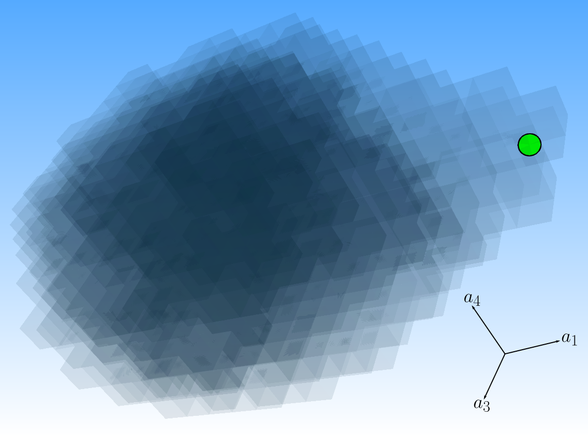 Figure 1
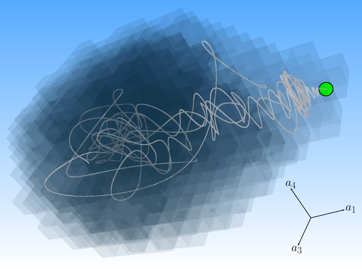 Figure 2
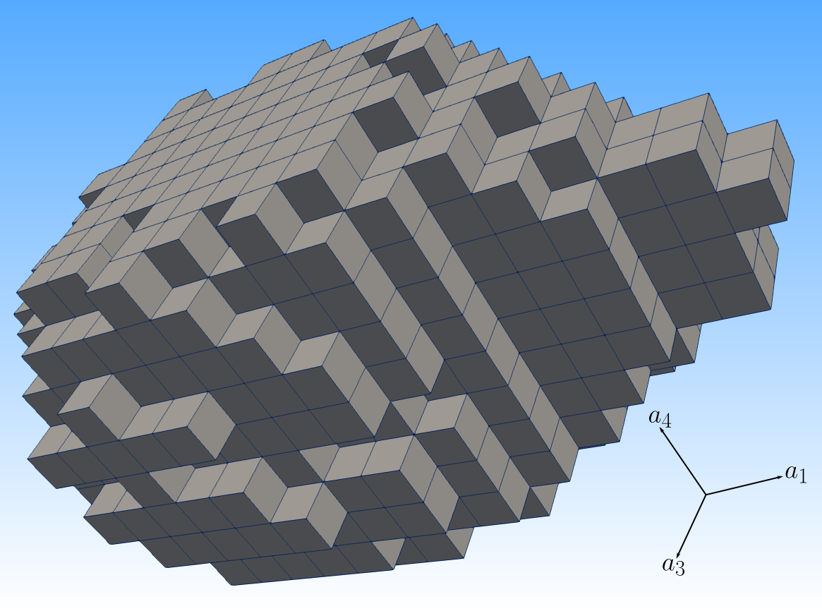 Figure 3
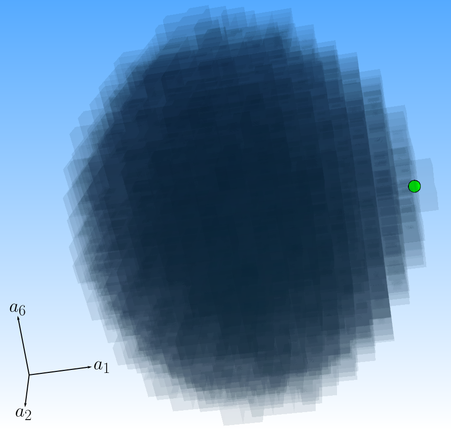 Figure 4
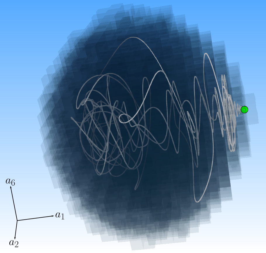 Figure 5
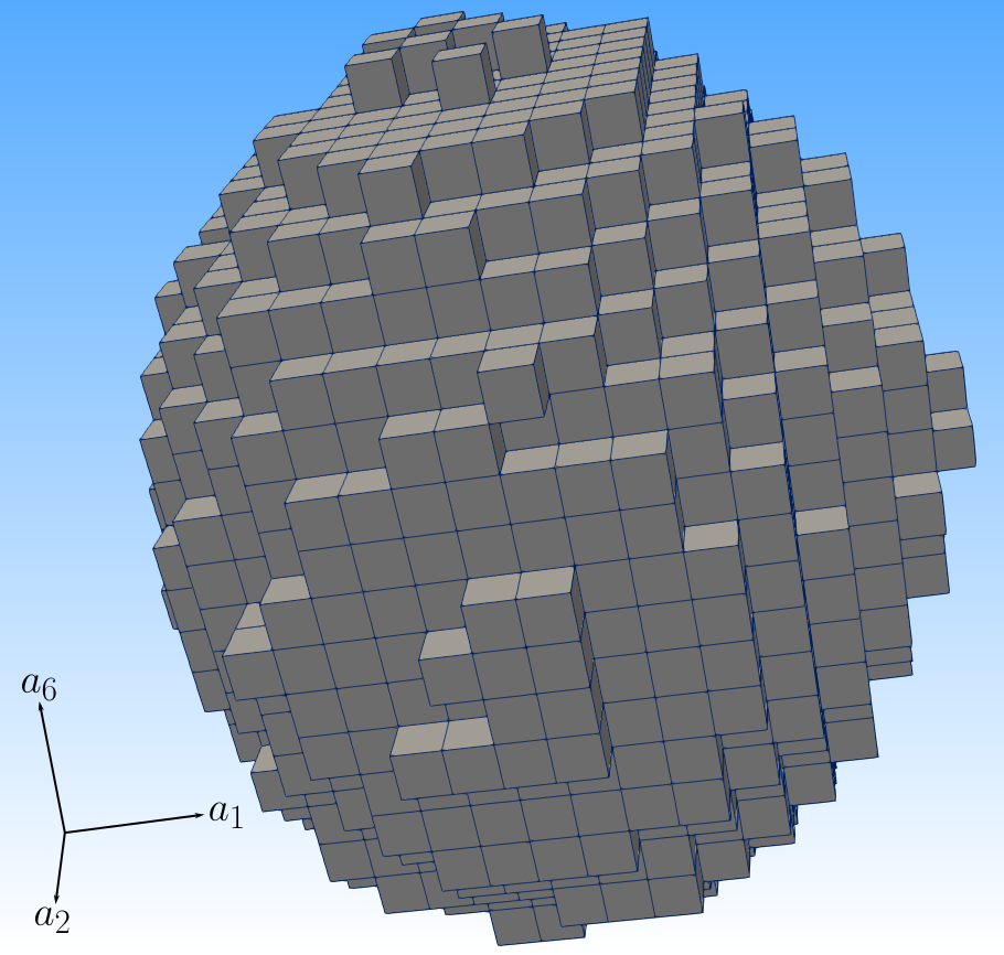 Figure 6
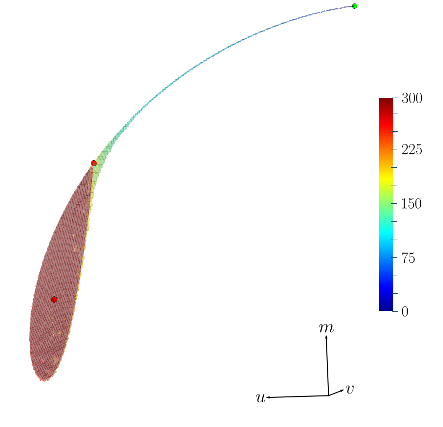 Figure 7
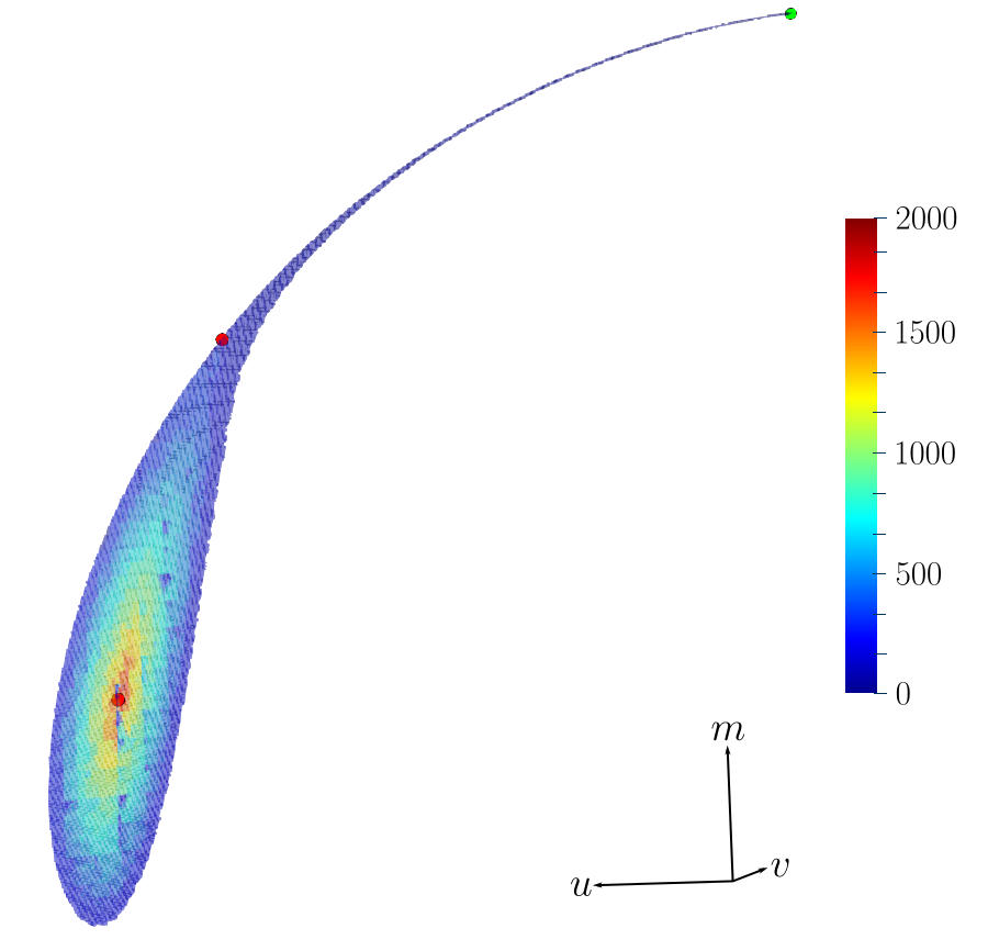 Figure 8
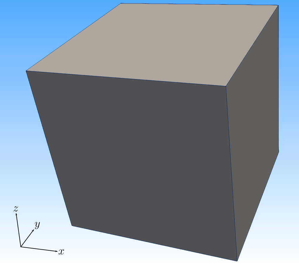 Figure 9
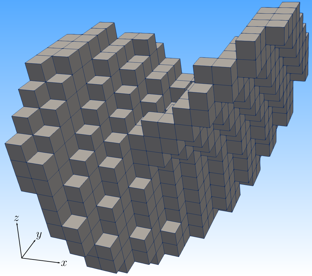 Figure 10
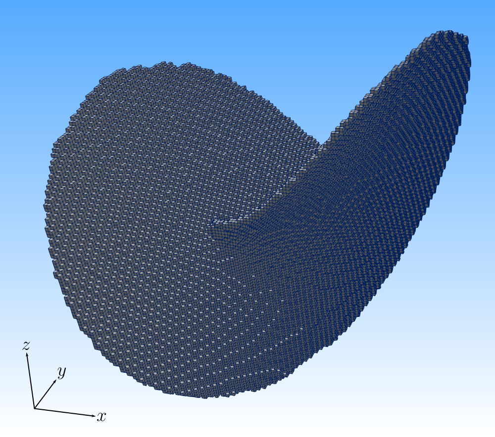 Figure 11
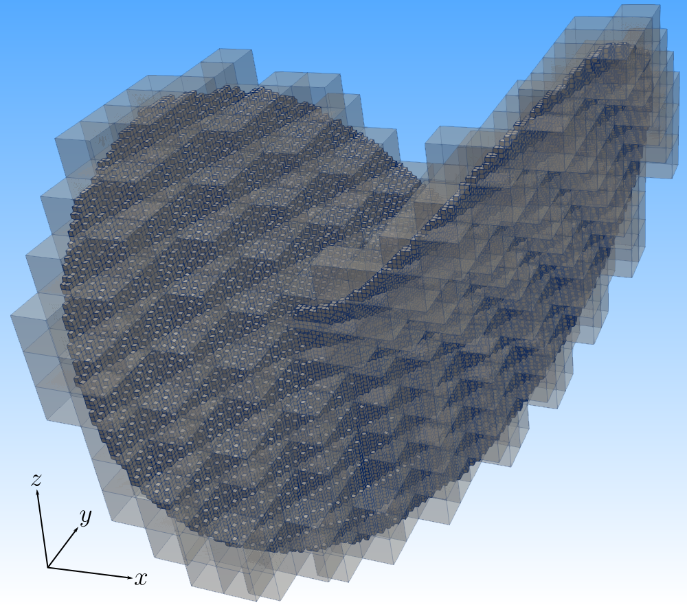 Figure 12
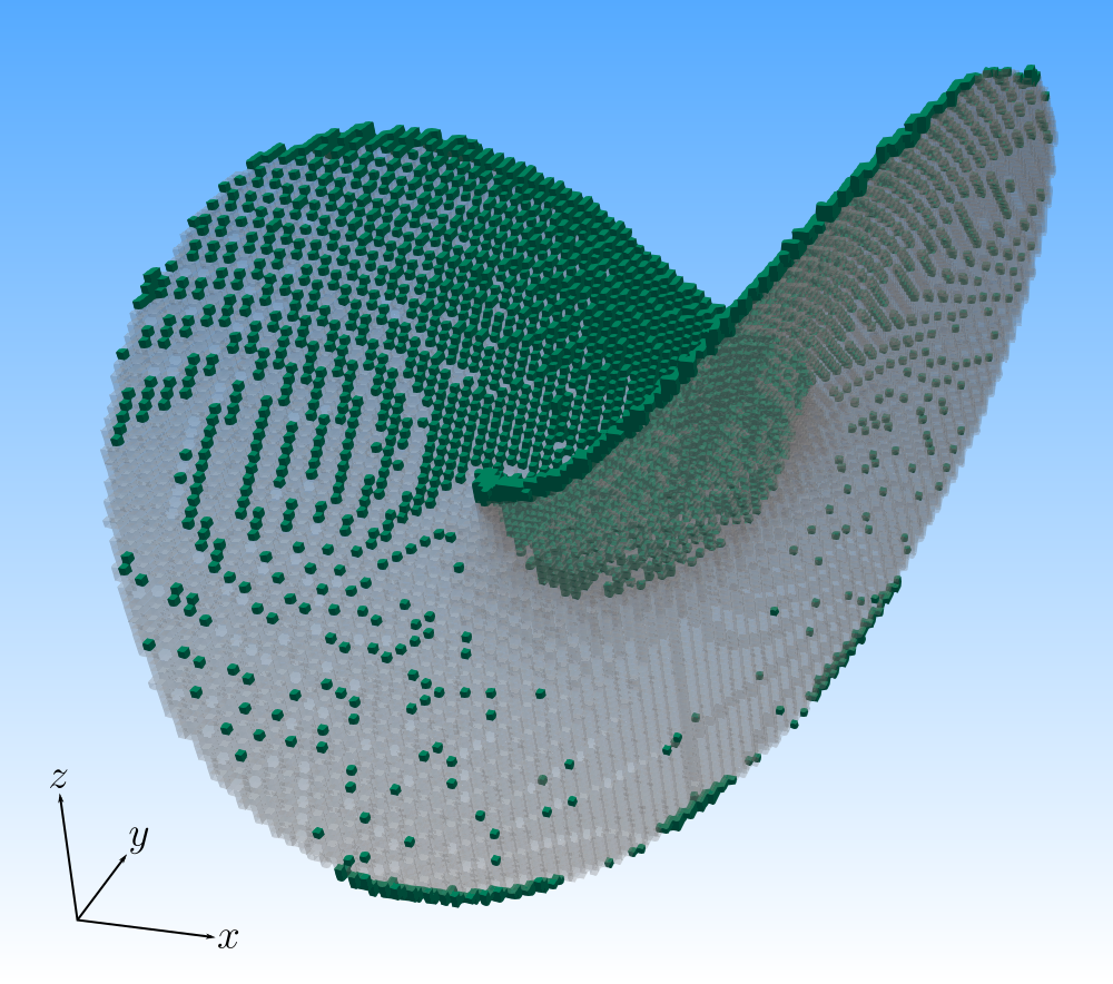 Figure 13
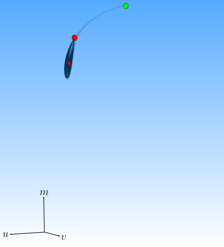 Figure 14
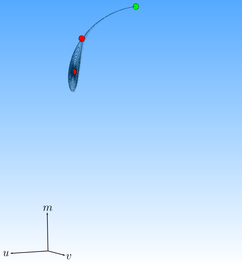 Figure 15
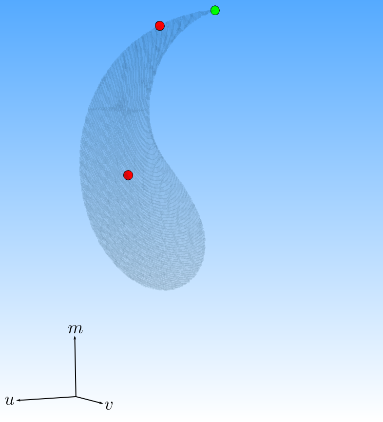 Figure 16
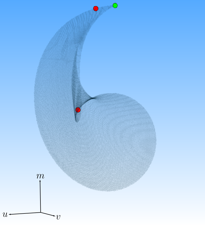 Figure 17
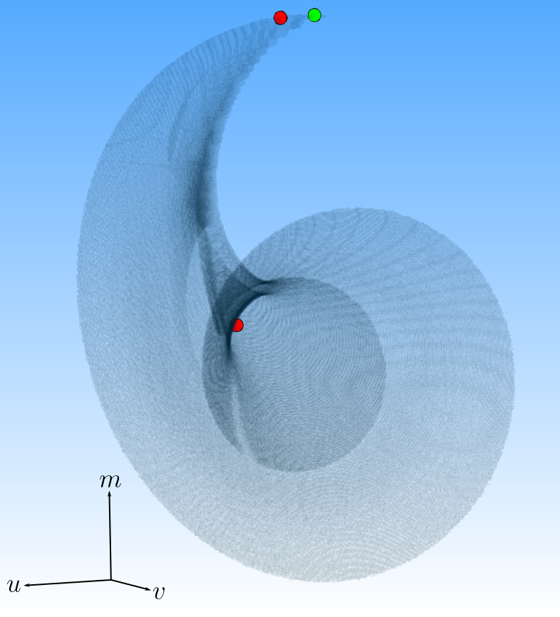 Figure 18
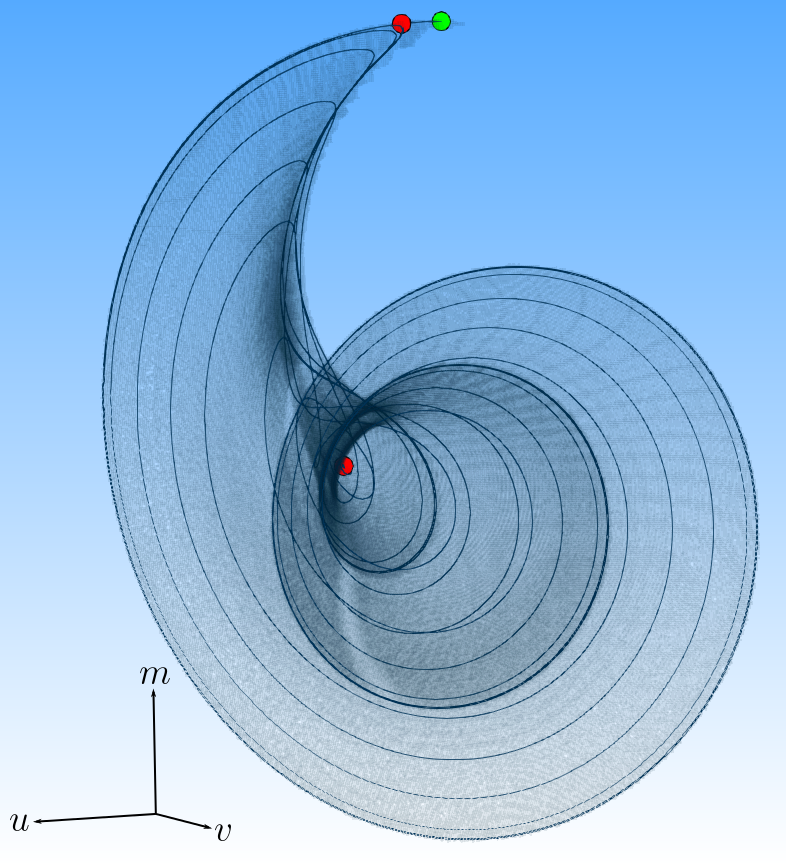 Figure 19
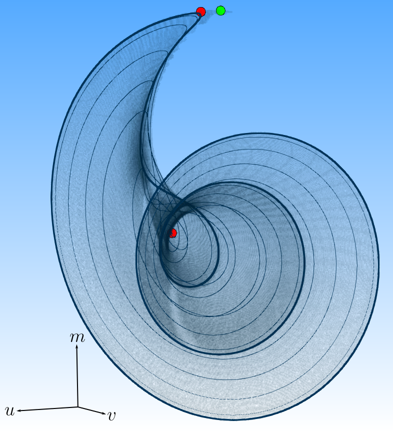 Figure 20
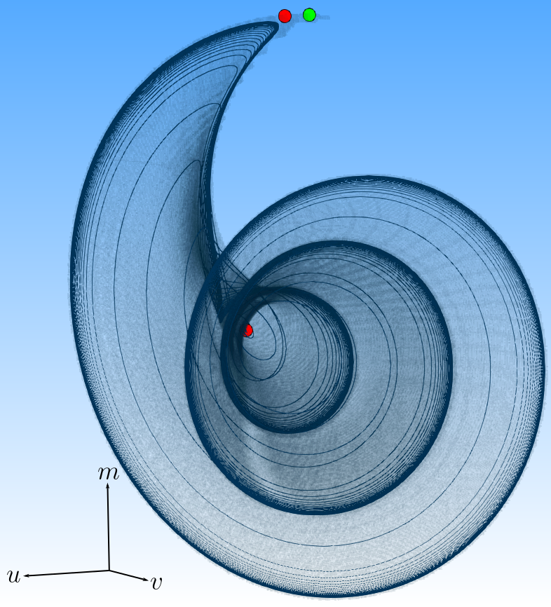 Figure 21
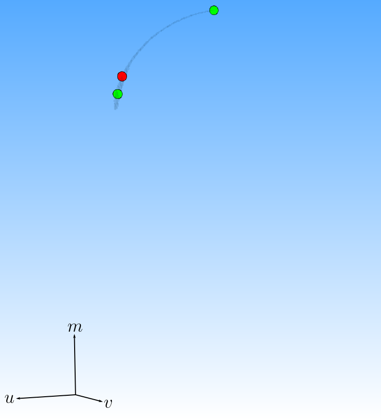 Figure 22
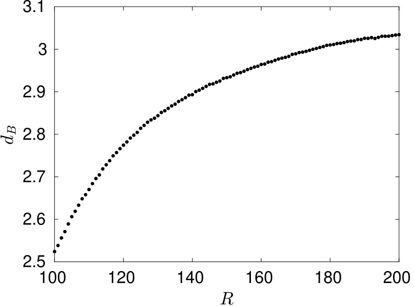 Figure 23
Peer Reviews
No public reviews on file for this paper yet. If you reviewed it on a platform where reviews are public (OpenReview, ICLR, NeurIPS, ICML), you can paste yours below so the community can read it here.
Videos
No videos yet. Explain this paper in a talk, walkthrough, or lecture? Add one.
Taxonomy
TopicsFluid Dynamics and Turbulent Flows · Model Reduction and Neural Networks · Quantum chaos and dynamical systems
A set-oriented path following method for the approximation of parameter dependent attractors
Raphael Gerlach
Department of Mathematics, Paderborn University, 33098 Paderborn, Germany.
Adrian Ziessler
Department of Mathematics, Paderborn University, 33098 Paderborn, Germany.
Bruno Eckhardt
Fachbereich Physik, Philipps-Universität Marburg, 35032 Marburg, Germany.
Michael Dellnitz
Department of Mathematics, Paderborn University, 33098 Paderborn, Germany.
Abstract
In this work we present a set-oriented path following method for the computation of relative global attractors of parameter-dependent dynamical systems. We start with an initial approximation of the relative global attractor for a fixed parameter computed by a set-oriented subdivision method. By using previously obtained approximations of the parameter-dependent relative global attractor we can track it with respect to a one-dimensional parameter without restarting the whole subdivision procedure. We illustrate the feasibility of the set-oriented path following method by exploring the dynamics in models for shear flows during the transition to turbulence.
1 Introduction
Over the last two decades so-called set-oriented numerical methods have been developed in the context of the numerical treatment of finite dimensional dynamical systems (e.g., [12, 13, 14, 27, 29]). Here, the basic idea is to cover the objects of interest such as attractors, invariant manifolds or almost invariant sets by outer approximations which are created via subdivision and continuation techniques. The numerical effort depends essentially on the dimension of the global attractor, i.e., it is easier to compute a one-dimensional attractor in a ten-dimensional space than to compute a three-dimensional attractor in a four-dimensional space [13]. The set-oriented techniques have been used successfully in several different application areas such as molecular dynamics ([19, 46, 10]), astrodynamics ([17, 16, 15]) and ocean dynamics ([28]). Moreover, a set-oriented numerical framework has recently been developed which allows to perform uncertainty quantification for dynamical systems from a global point of view [18] and the computation of finite dimensional attractors or unstable manifolds of infinite dimensional dynamical systems [11, 52, 51]. In this work we connect these set-oriented algorithms with ideas from bifurcation analysis and path following methods in order to efficiently treat parameter dependencies in the underlying dynamical system.
Systems of physical interest typically depend on parameters appearing in the defining systems of equations, i.e., one considers dynamical systems of the form
[TABLE]
where are the variables, are the system parameters, and is assumed to be sufficiently smooth. By varying , the qualitative structure of the solutions might change significantly, e.g., stable equilibria of the dynamical system might become unstable. Such phenomena are known as bifurcations and the parameter values are called bifurcation parameters (see [34, 36, 32, 49] for a detailed overview).
Bifurcations typically come in two kinds. On the one hand, one can look at local bifurcations [34, 32], where the analysis of such bifurcations is generally performed by studying the corresponding vector fields near equilibrium points. That is, one can usually reduce the problem to the analysis of an equation of the form
[TABLE]
Starting with an initial the aim is to find numerically an approximation of a solution curve depending on which is implicitly defined by (2). The basic idea of path following methods which tackle this kind of problem for parameter-dependent fixed points and steady states can be found, e.g., in [1] and [2]. For the numerical treatment of bifurcation problems there exist a wide range of software tools, e.g., the well-known software package AUTO [21]. A first-version of AUTO has already been developed in 1981. More recent contributions to bifurcation analysis software are the MATLAB packages MATCONT [20] and COCO [7].
On the other hand, there are global bifurcations [31, 49] for which it is not sufficient to reduce the study to a neighborhood of an equilibrium or a fixed point. For example, these bifurcations occur when invariant sets, such as periodic orbits, collide with equilibria. Therefore, typical examples are formations of homoclinic and heteroclinic orbits which can also be found numerically with the software package AUTO [21] and COCO by formulating and solving an appropriate boundary value problem (e.g., [22]). In addition, MATCONT is able to continue homoclinic and heteroclinic orbits by a homotopy method [8].
In this work we extend the subdivision method for the approximation of the so–called relative global attractor to parameter-dependent dynamical systems, i.e., we design a path following method from a global point of view, which indirectly allows the numerical analysis of global bifurcations. Note that the relative global attractor contains all backward invariant sets and, in particular, the homoclinic or heteroclinic connections. Using previously obtained approximations of the relative global attractor we can track it with respect to a one-dimensional parameter without restarting the whole subdivision procedure. Since one computation of an attracting set might be very expensive by using the set-oriented method, the algorithm developed in this article can reduce the overall computational cost significantly. The set-oriented path following algorithm has been implemented in the dynamical systems software package GAIO (Global Analysis of Invariant Objects) [9], which is available for MATLAB (see https://github.com/gaioguy/GAIO).
We will use the set-oriented path following method to explore the dynamics of shear flows during the transition to turbulence. In contrast to convection or Taylor-Couette flows, where the transition can be captured by sequences of bifurcations that branch off the laminar state [4, 5], shear flows such as pipe flow or plane Couette flow do not show a linear instability of the laminar profile [45, 33]. The transition is then mediated by the presence of 3d states that form in saddle-node bifurcations [44, 24, 23, 25]. Very close to the bifurcation, the states of the upper branches can be stable, but they soon undergo secondary bifurcations and period doubling cascades [39, 3, 50]. Crisis bifurcations destroy the attractors and give rise to the open saddles that underlie the observed transience of the turbulent state [38, 40].
Exploring the dynamics in the full phase space is very complicated because of the high-dimensionality of the relevant subspaces, though notable progress has been made in some cases [35, 30]. In order to prepare for the application to such computationally expensive examples, we begin here with an analysis of simple models that capture much of the phenomenology of shear flows: they have a laminar state that is linearly stable and a saddle-node bifurcation that represents the transition to turbulence. The models even contain the transition from an attractor to a transient saddle.
The simplest model where the modes have a physical interpretation is the four-dimensional model proposed by Waleffe [47]: the four components represent the transversal velocity components, the vortices, the streak, and the mean velocity. With the methods described here, we are able to trace the appearance of the attractor and its growth as the Reynolds number increases. We will then extend the analysis to the case of the nine-dimensional model discussed in [42, 43].
A detailed outline of the paper is as follows: in Section 2.1 we briefly summarize the subdivision method introduced in [13]. In Section 2.2 we then develop the set-oriented path following method which allows us to compute attracting sets of parameter-dependent dynamical systems without restarting the subdivision procedure. In Section 3 we illustrate the efficiency of the path following method for two different reduced order models from fluid dynamics, namely, a four-dimensional model of self-sustained flows and a nine-dimensional model of turbulent shear flows. Conclusions are given in Section 4.
2 A set-oriented path following method
We consider parameter dependent dynamical systems of the form
[TABLE]
where and is a homeomorphism for each parameter in an open subset and uniformly continuous in on bounded sets, e.g., could be a time--map for the system (1). In what follows, for fixed we use the abbreviation . Moreover, we assume that has a compact global attractor for each , that is, the compact set attracts any bounded set . Later on, we will additionally assume that is upper semi-continuous in .
The aim of this work is to develop a set-oriented path following method for the approximation of depending on the parameter . Since this method is based on the framework developed in [13] we start with a short review of the related material.
2.1 Brief review of the subdivision method
Let be a compact set. For a homeomorphism we define the global attractor relative to by
[TABLE]
Observe that if is the compact global attractor of .
As a first step we approximate this set with a subdivision procedure introduced in [13] for a fixed , that is, . Roughly speaking, the idea of the algorithm is to start with a finite family of compact subsets of that are a partition of . Then we refine this partition and remove those subsets that do not contain parts of the relative global attractor. By continuing this process we generate a sequence of finite collections of compact subsets of such that the diameter
[TABLE]
converges to zero and the union approaches the relative global attractor for .
More precisely, let be the initial collection, e.g., . Then we inductively obtain from for in two steps.
Subdivision: Construct a new collection such that
[TABLE]
and
[TABLE]
where . 2. 2.
Selection: Define the new collection by
[TABLE]
The first step guarantees that the collections consist of successively finer sets for increasing . In fact, by construction
[TABLE]
In the second step we remove each subset whose preimage does neither intersect itself nor any other subset in .
Remark 2.1**.**
In the application of the subdivision scheme for the computation of the relative global attractor we have to perform the selection step
[TABLE]
Thus, we have to decide whether or not the preimage of a given set has a nonzero intersection with another set , i.e.,
[TABLE]
Numerically this is realized as follows: we discretize each box by a finite set of test points and replace the condition (5) by
[TABLE]
The selection step is responsible for the fact that the unions approach the relative global attractor. Denote by the collection of compact sets obtained after subdivision steps, that is
[TABLE]
Note that these sets form a nested sequence . Therefore the limit
[TABLE]
exists and the following result has been proven in [13]:
Proposition 2.2**.**
Let be the global attractor relative to , and let be a finite collection of closed subset with . Then the sets obtained by the subdivision algorithm contain the relative global attractor, for all , and moreover
[TABLE]
2.2 Path following method for the approximation of relative global attractors
In this section we develop a path following algorithm that allows to compute the relative global attractor for various parameter values of (3) by reusing previously obtained coverings. The idea of this method is to first approximate the relative global attractor for and then to use a covering of this set, denoted by , as a starting point to compute the relative global attractor for sufficiently close to .
We start with the following observation.
Lemma 2.3**.**
Let be a homeomorphism and assume that has a compact global attractor . Furthermore, let be compact sets such that . Then,
[TABLE]
where is the global attractor relative to for .
Proof.
This statement follows directly by the definition of the global attractor relative to a compact set (cf. (4)) and the fact that . ∎
As a direct consequence we obtain the following result.
Proposition 2.4**.**
Let be a homeomorphism and assume that has a compact global attractor . Let be compact sets such that and denote by , , the corresponding sets obtained after subdivision and selection steps (see (6)). Then
[TABLE]
where denotes the usual Hausdorff distance between two compact subsets .
Proof.
This result is a direct consequence of Proposition 2.2 and Lemma 2.3. ∎
Proposition 2.4 states that by performing sufficiently many subdivision and selection steps we obtain a good approximation of the attracting set no matter how we choose the initial covering as long as .
In what follows, let us assume that is a compact set such that for all . We denote by a finite family of compact sets , , which all contain the global attractor relative to of the map . Next, either we fix and choose sufficiently small such that or we fix and choose sufficiently close to such that . In any case Lemma 2.3 and Proposition 2.4 allows us to approximate the global attractor of the map using the initial covering with the subdivision algorithm described in the previous section. Observe that we can always choose for every , since and for by assumption.
To discuss the choice of for fixed we have to analyze the change of the attractor when the parameter is varied. To this end, we define the distance between two subsets of as
[TABLE]
This distance allows us to define the continuity of attractors as follows:
Definition 2.5**.**
Let . The family of attractors is upper semi-continuous at if
[TABLE]
The attractor is called upper semi-continuous if is upper semi-continuous for each .
Note that upper semi-continuity at implies that for every there exists a neighborhood of such that for all , where denotes the -neighborhood of . Thus, the attractor cannot become larger instantaneously by varying which is a naturally needed property for our proposed path following scheme. In fact, if the attracting set suddenly “explodes” we cannot assure that any previously computed covering besides still covers . For the sake of completeness we note that lower semi-continuity of , i.e.,
[TABLE]
prevents a sudden shrinking of which holds for instance for gradient systems with hyperbolic fixed points [37]. However, this would be, in general, no issue for our proposed algorithm.
We are now in the position to prove that for each there is a range of parameters such that the attractor can be approximated by the subdivision algorithm with the initial compact set .
Proposition 2.6**.**
Let be the family of sets generated by the subdivision method such that for all . Suppose that there is such that for all and is upper semi-continuous at . Then for every there exists such that for all . In particular, can be approximated by using the initial compact set .
Proof.
Let be fixed. Due to the upper semi-continuity of in there is such that
[TABLE]
Thus, we conclude by assumption that
[TABLE]
∎
In the following we will call such feasible and Proposition 2.6 guarantees the existence of a feasible . Throughout the remainder of this article we now suppose that is upper semi-continuous and the additional assumptions of Proposition 2.6 hold. Then the numerical realization of the set-oriented path following algorithm can be described as follows:
In Figure 1, we illustrate two steps of Algorithm LABEL:alg:pathFollowing for the Lorenz system [41] given by
[TABLE]
where we use as our parameter of interest. We note that the derivation of the Lorenz model shows that is related to the aspect ratio of the convection cells.
Remark 2.7**.**
- (a)
Instead of following the path along in positive direction one can also take and follow the path in the negative direction. 2. (b)
Intuitively, choosing a larger decreases the range of feasible parameters . However, one has to perform less subdivision and selection steps to reach the same level, i.e., the same fineness of the final box covering of . With more knowledge on the upper semi-continuity property (7) we can make this more precise in the following Proposition. 3. (c)
If is not feasible, i.e., , might not contain all of and thus, the subdivision algorithm does not approximate the whole attractor . However, to make the algorithm more robust, we reintroduce sets if an image of a test point is not contained in any set of the current collection .
After discussing the choice of for fixed the following Proposition tells us, how to choose for a fixed step size in the parameter space , i.e., how to choose when is given.
Proposition 2.8**.**
Let and with . Suppose there is a constant such that
[TABLE]
and for one . Then and, in particular, is feasible for .
Proof.
According to (9) the -neighborhood of contains and by assumption we immediately obtain
[TABLE]
as claimed. ∎
3 Numerical examples
In this section we present results of computations carried out for a four- and a nine-dimensional reduced order model from fluid dynamics.
3.1 A four-dimensional model of self-sustained flows
As a first example, we consider a four-dimensional nonlinear model of self-sustained flows introduced in [47] and further discussed in [48]. The four variables of the model represent the spanwise velocity components (), the vortices (), the streak (), and the mean profile () (cf. [48] for more explanations of the model). Their dynamics is given by
[TABLE]
where is the Reynolds number, and , , , , and are positive parameters. For the parameters, we take values , , and ; a saddle-node bifurcation then appears for .
Our goal is to numerically analyze how the attracting sets change for the Reynolds numbers . We define and denote by the time--map of (10) which depends on the Reynolds number and the integration time . For the following analysis we fix the integration time of . Furthermore, we choose the initial box in which we want to approximate the relative global attractor . According to Algorithm LABEL:alg:pathFollowing we fix and . Following of Remark 2.7 (a) we start the path following algorithm for the Reynolds number and define for such that the interval is discretized equidistantly. A detailed analysis of (10) for can be found in [48]. In what follows, we will study the attractor from a global point of view. To this end, Figure 2 and Figure 4 show three-dimensional projections of the relative global attractor obtained by Algorithm LABEL:alg:pathFollowing for different Reynolds numbers.
For a parameter value just below the saddle-node bifurcation, i.e., for , the attracting set does not contain any invariant structures besides the laminar profile . For just above the saddle node bifurcation, i.e., for , Figure 2 (a) shows that the attractor now contains an upper branch steady solution, as well as the lower branch saddle state. This situation persists up to , after which the upper branch undergoes a supercritical Hopf bifurcation.
The limit cycle is stable (cf. Figure 2 (b)) until (cf. Figure 2 (c)), where it disappears in a homoclinic bifurcation. Note that the attracting set does not change significantly, although the dynamics does: in the homoclinic bifurcation the attractor rips open and becomes a transient saddle. In order to demonstrate this change in the dynamics, we compare in Figure 3 (a) and (b) the average lifetimes for each box in the attracting set for and , respectively.
For we see a strict separation in the attracting set by the edge state: all boxes between the edge state and the laminar state have finite lifetimes, as they are attracted towards the laminar profile. All boxes inside the lobe around the upper branch state have infinite lifetimes because they are attracted to the limit cycle and cannot return to the laminar profile. Here, test points in each box were only integrated for times up to : the choice of time is not essential, since for a closed attractor around the upper branch state no trajectory can return to the laminar flow. For the limit cycle is not stable anymore, and all points except for the fixed points and the limit cycle return to the laminar profile. Observe that the obtained box coverings do not only cover the laminar profile but also the unstable manifolds which is due to the fact that the relative global attractor contains all backward invariant sets.
For the attractor develops a more complicated structure with folds and other features (Figure 4 (a–d)), that arise from the projection from the four-dimensional state space to the three-dimensional image plane.
Finally, for another stable limit cycle appears (cf. Figure 4 (e) and (f)).
3.2 A nine-dimensional model for turbulent shear flows
As a second example we consider a Fourier based nine-dimensional model for a turbulent shear flow with free slip boundaries and a sinusoidal base profile. A first version with 8 degrees of freedom was described by Waleffe [47, 48], and extended to 9 modes in [42, 43]. The model is based on a Fourier expansion of the velocity field, and every component can be assigned to a specific flow field. In addition to the Reynolds number, the model has two spatial parameters describing the domain size in spanwise and downstream direction. The choice we consider here is the NBC domain (Nagata, Busse, Clever [44, 6]), i.e., a box with in spanwise and in downstream direction. For these parameters, the first state that appears is a periodic orbit, at . The periodic orbit is unstable from the onset, so that the dynamics is transient without the need for the occurrence of a crisis bifurcation. However, the lifetime increases very rapidly with Reynolds number [42].
Again, we choose the Reynolds number as our parameter of interest and compute the relative global attractor for Reynolds numbers starting with an initial and then decreasing in steps of one, , . Due to the complexity of the dynamics in the nine-dimensional phase space it is hard to visualize the attracting set. An impression of the set may be obtained by three-dimensional projections onto the modes that correspond to in the four-dimensional model (10) and to the modes which represent the principal components of the set.
In Figure 5 we see that these projections of the attractor look like dense balls with no discernable interior structure. A measure of the increasing complexity of the dynamics is the dimension of the attracting set, here quantified by the box-counting dimension (cf. [26]) of the box coverings obtained by Algorithm LABEL:alg:pathFollowing. Figure 6 shows that this dimension increases with Reynolds number. For the dimension of the attracting set is about and increases to about for and most likely even higher values for .
4 Conclusions
The set-oriented path following method is a powerful tool for the numerical analysis of global bifurcations for attracting sets. With the method developed in this paper the actual covering of an attracting set for a parameter value can be used as an initial covering for a parameter which is sufficiently close to . Thus, we do not need to restart the subdivision method, thereby significantly reducing the overall computational time. However, this path following method is only defined for finite dimensional dynamical systems. Therefore, it should be desirable to extend this work to the infinite dimensional setting, i.e., for the parameter dependent computation of attractors of infinite dimensional dynamical systems. In this context the results of [11, 52, 51] would have to be adapted.
The results in this article show that set-oriented methods can also be used in moderate-dimensional settings, where they can provide insight into the dynamics of shear flows during the transition to turbulence in simple models. The similarities in the behaviour of the low-dimensional models and fully resolved numerical simulations suggests that the global organization of phase space will be similar, even though such a study is computationally out of reach for high-dimensional attractors.
Acknowledgments
This work is supported by the Priority Programme SPP 1881 Turbulent Superstructures of the Deutsche Forschungsgemeinschaft.
The reference list from the paper itself. Each links out to its DOI / PubMed record.
- 1[1] E. L. Allgower and K. Georg. Continuation and path following. Acta numerica , 2:1–64, 1993.
- 2[2] E. L. Allgower and K. Georg. Numerical path following. Handbook of numerical analysis , 5:3–207, 1997.
- 3[3] M. Avila, F. Mellibovsky, N. Roland, and B. Hof. Streamwise-Localized Solutions at the Onset of Turbulence in Pipe Flow. Phys Rev Lett , 110(22):224502, May 2013.
- 4[4] S. Chandrasekhar. Hydrodynamic and hydromagnetic stability . Oxford University Press, Oxford, 1961.
- 5[5] P. Chossat and G. Iooss. The Couette-Taylor Problem . Springer-Verlag, 1994.
- 6[6] RM Clever and Fritz H Busse. Tertiary and quaternary solutions for plane couette flow. Journal of Fluid Mechanics , 344:137–153, 1997.
- 7[7] H. Dankowicz and F. Schilder. Recipes for continuation , volume 11 of Computational Science and Engineering . SIAM, 2013.
- 8[8] V. De Witte, W. Govaerts, Y. A. Kuznetsov, and M. Friedman. Interactive initialization and continuation of homoclinic and heteroclinic orbits in matlab. ACM Transactions on Mathematical Software (TOMS) , 38(3):18, 2012.