Finite element method for radially symmetric solution of a multidimensional semilinear heat equation
Toru Nakanishi, Norikazu Saito

TL;DR
This paper develops and analyzes a finite element method for solving radially symmetric solutions of multidimensional semilinear heat equations, providing error estimates and validating results through numerical examples.
Contribution
It introduces optimal error estimates for finite element solutions of semilinear heat equations with radial symmetry, including both symmetric and nonsymmetric formulations.
Findings
Optimal order error estimates in $L^ Infty$ and weighted $L^2$ norms.
Validation of theoretical results through numerical examples.
Abstract
This study aims to present the error and numerical blow up analyses of a finite element method for computing the radially symmetric solutions of semilinear heat equations. In particular, this study establishes optimal order error estimates in and weighted norms for the symmetric and nonsymmetric formulation, respectively. Some numerical examples are presented to validate the obtained theoretical results.
Click any figure to enlarge with its caption.
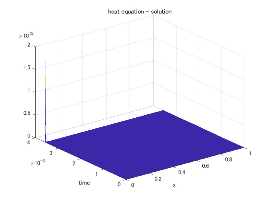 Figure 1
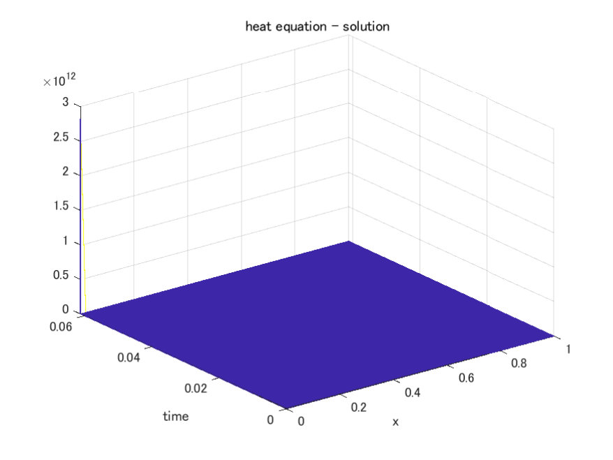 Figure 3
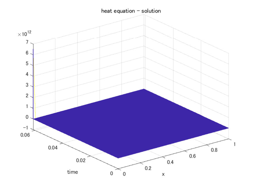 Figure 4
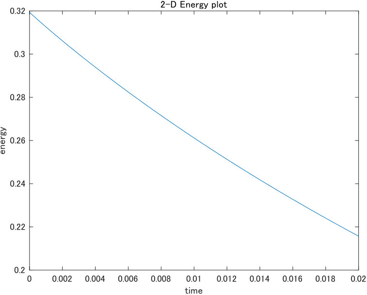 Figure 7
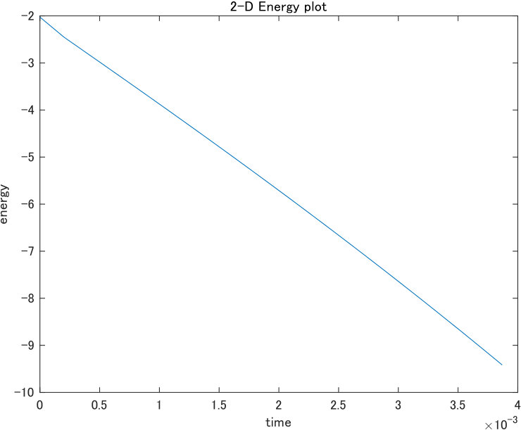 Figure 8
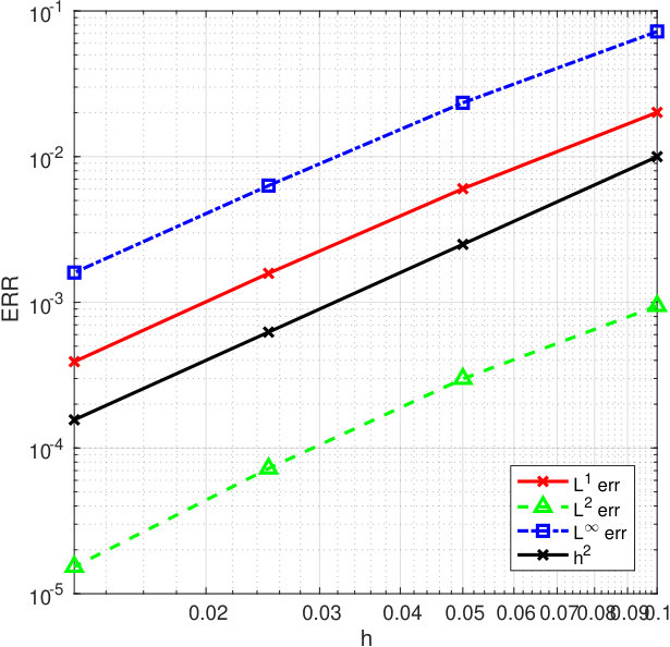 Figure 6
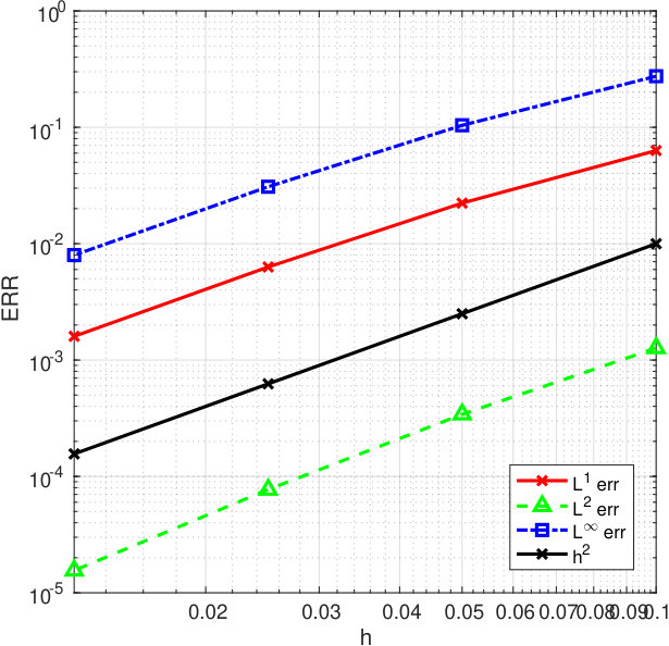 Figure 7
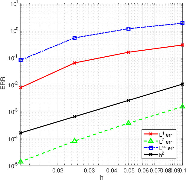 Figure 8
 Figure 1
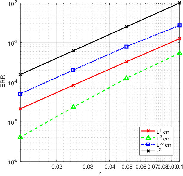 Figure 10
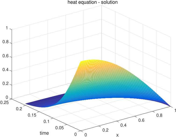 Figure 2
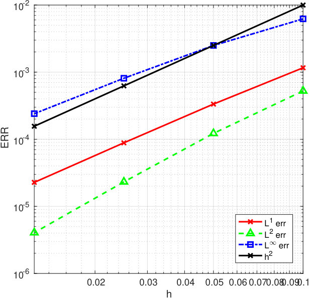 Figure 9
Peer Reviews
No public reviews on file for this paper yet. If you reviewed it on a platform where reviews are public (OpenReview, ICLR, NeurIPS, ICML), you can paste yours below so the community can read it here.
Videos
No videos yet. Explain this paper in a talk, walkthrough, or lecture? Add one.
Taxonomy
TopicsAdvanced Numerical Methods in Computational Mathematics · Numerical methods for differential equations · Numerical methods in engineering
Finite element method for radially symmetric solution of a multidimensional semilinear heat equation
Toru Nakanishi Graduate School of Mathematical Sciences, The University of Tokyo, Komaba 3-8-1, Meguro-ku, Tokyo 153-8914, Japan. E-mail: [email protected], TEL 81-3-5465-7001, FAX 81-3-5465-7011
Norikazu Saito Graduate School of Mathematical Sciences, The University of Tokyo, Komaba 3-8-1, Meguro-ku, Tokyo 153-8914, Japan. E-mail: [email protected], TEL 81-3-5465-7001, FAX 81-3-5465-7011
Abstract
This study was conducted to present error analysis of a finite element method for computing the radially symmetric solutions of semilinear heat equations. Particularly, this study establishes optimal order error estimates in and weighted norms, respectively, for the symmetric and nonsymmetric formulation. Some numerical examples are presented to validate the obtained theoretical results.
Key words:
finite element method, numerical analysis, radially symmetric solution, semilinear parabolic equation
2010 Mathematics Subject Classification: 65M60, 35K58,
1 Introduction
This study was conducted to investigate the convergence property of finite element method (FEM) applied to a parabolic equation with singular coefficients for the function , , and , as expressed in
[TABLE]
where is a given locally Lipschitz continuous function, is a given continuous function, and
[TABLE]
is a given parameter.
In the study of an -dimensional semilinear heat equation, the following problem arises as
[TABLE]
where represents a bounded domain in . If one is concerned with the radially symmetric solution in the -dimensional ball \Omega=\{\bm{x}\in\mathbb{R}^{N}\mid|\bm{x}|=|\bm{x}|_{\mathbb{R}^{N}}{\color[rgb]{0,0,0}<}1\}, then (3) implies (1), where and .
For a linear case in which is replaced by a given function , the works [7, 15] studied the convergence property of the FEM to (1) along with the corresponding steady-state problem, and two proposed schemes: the symmetric scheme, wherein they established the optimal order error estimate in the weighted norm ; and the nonsymmetric scheme, wherein they proved the error estimate. In this paper, both schemes are applied to the semilinear equation (1) to derive various error estimates. Moreover, this study includes a discussion of discrete positivity conservation properties, which earlier studies [7, 15] failed to embrace, but which are actually important in the study of diffusion -type equations.
Our emphasis is on FEM because we are able to use non-uniform partitions of the space variable . Therefore, the method is deemed useful for examining highly concentrated solutions at the origin. On this connection, we present our motivation for this study. The critical phenomenon appearing in the semilinear heat equation of the form
[TABLE]
in a multidimensional space has attracted considerable attention since the pioneering work of Fujita [8]. According to him, the equation is in the whole dimensional space . Any positive solution blows up in a finite time if , whereas a solution is smooth at any time for a small initial value if . Therefore, expression is known as Fujita’s critical exponent ( [11, 6] provides some critical exponents of other equations). Generally, similar critical exponents can be found for an initial-boundary value problem for the semilinear heat equation . Some examples are given in reports of earlier studies [9, 11, 6]. However, the concrete values of those critical conditions are apparently unknown. Therefore, we found it interesting to study the numerical methods for computing the solutions of nonlinear partial differential equations in an -dimensional space. However, computing the non-stationary four-space dimensional problem is difficult, even for modern computers. We consider the FEM to solve the one space dimensional equation (1). However, we face another difficulty in dealing with the singular coefficient , which the FEM reasonably simplified, as explained later.
As described above, the main purpose of this paper is to derive various optimal order error estimates for the symmetric and nonsymmetric schemes of [7, 15] applied to (1). These schemes are described below as (Sym) and (Non-Sym). To this end, we address mostly the general nonlinearity . Moreover, we study discrete positivity conservation properties. We summarize our typical results here.
- •
The solution of (Sym) is positive if and if the discretization parameters satisfy some conditions, as shown by Theorem 3.2.
- •
If is a globally Lipschitz continuous function, then the solution of (Sym) converges to the solution of (1) in the weighted norm for the space and in the norm for time. Moreover, the convergence is at the optimal order, as shown by Theorem 4.1.
- •
If is a locally Lipschitz continuous function and , then the solution of (Sym) converges to the solution of (1) in the weighted norm for the space and in the norm for time. The convergence is at the optimal order, as shown by Theorem 4.3.
- •
If with and if the time partition is uniform, then the solution of (Non-Sym) converges to the solution of (1) in the norm. The convergence is at the optimal order up to the logarithm factor, as shown by Theorem 4.6.
However, we do not proceed to applications of our schemes to the blow-up computation in this work. In fact, from the main results presented in this paper, we infer that the standard schemes of [7, 15] do not fit for the blow-up computation for large . For the symmetric scheme, the restriction reduces interest in considering radially symmetric problems. Moreover, for the nonsymmetric scheme, the use of uniform time-partitions makes it difficult to apply Nakagawa’s time-partitions control strategy: a powerful technique for computing the approximate blow-up time, as described in earlier reports [3, 12, 14, 5, 4, 13, 2]. Nevertheless, we believe that our results are of interest to researchers in this and related fields. In fact, the validity issue of the symmetric scheme only for was pointed out earlier in [1] for a nonlinear Schrödinger equation with no mathematical evidence. The analysis reported herein reveals weak points of the two standard schemes. As a sequel to this study, we propose a new finite element scheme for (1). The scheme, which uses a nonstandard mass-lumping approximation, is shown to be positivity-preserving and convergent for any . Details will be reported in a forthcoming paper.
It is noteworthy that the finite difference method for (1) has been studied and that its optimal order convergence was proved in an earlier report [3]. Its finite difference scheme uses a special approximation around the origin to assume a uniform spatial mesh.
This paper comprises five sections. Section 2 presents our finite element schemes. Well-posedness and positivity conservation are examined in Section 3. Section 4 presents the error estimates and their proofs. Finally, Section 5 presents some numerical examples that validate our theoretical results.
2 Finite element method
First, we derive two alternate weak formulations of (1). Unless otherwise stated explicitly, we assume that is a locally Lipschitz continuous function such that
[TABLE]
Letting be arbitrary, then multiplying both sides of (1a) by and using integration by parts over , we obtain
[TABLE]
Otherwise, if we multiply both sides of (1a) by instead of and integrate it over , then we have
[TABLE]
We designate (4) the symmetric weak form because of the symmetric bilinear form associated with the differential operator . In contrast, (5) is the nonsymmetric weak form. Both forms are identical at .
We now establish the finite element schemes based on these identities. For a positive integer , we introduce node points
[TABLE]
and set and , where . The granularity parameter is defined as . Let be the set of all polynomials in an interval of degree . We define the finite element space as
[TABLE]
Its standard basis function , j=0,1,\cdots,m{\color[rgb]{0,0,0},} is defined as
[TABLE]
where denotes Kronecker’s delta.
For time discretization, we introduce non-uniform partitions
[TABLE]
where denotes the time increments.
Generally, we write .
We are now in a position to state the finite element schemes to be considered.
(Sym) Find , , such that
[TABLE]
where is assumed to be given. Hereinafter, we set
[TABLE]
(Non-Sym) Find , such that
[TABLE]
where
[TABLE]
It is noteworthy that is coercive in such that
[TABLE]
3 Well-posedness and positivity conservation
In this section, we prove the following theorems.
Theorem 3.1** (Well-posedness of (Sym)).**
For a given with , the scheme (Sym) admits a unique solution .
Theorem 3.2** (Positivity of (Sym)).**
In addition to the basic assumption (f1), assume that
[TABLE]
Letting and , and assuming that
[TABLE]
then, the solution of (Sym) satisfies .
Theorem 3.3** (Comparison principle for (Sym)).**
We let and assume that satisfies in . Furthermore, we assume that (f1) and (f2) are satisfied. Similarly, we let be the solutions of (Sym) with , respectively, using the same time increment . Moreover, we assume that (12) is satisfied. Consequently, we obtain in . The equality holds true if and only if in .
Theorem 3.4** (Well-posedness of (Non-Sym)).**
For a given with , the scheme (Non-Sym) admits a unique solution .
To prove these theorems, we conveniently rewrite (7) into a matrix form. That is, we introduce
[TABLE]
and express (7) as
[TABLE]
where is understood as .
Lemma 3.5**.**
* and are both tri-diagonal and positive-definite matrices.*
Theorem 3.1 is a direct consequence of this lemma. We proceed to proofs of other theorems.
Proof of Theorem 3.2.
We use the representative matrix (13) instead of (7) and set
[TABLE]
If , then we obtain
[TABLE]
because and in view of (f2). The proof that is true under (12) is divided into three steps, each described as presented below.
Step 1. We show that
[TABLE]
Letting , we calculate
[TABLE]
because in . Cases and are verified similarly.
Step 2. We show that, if
[TABLE]
then . First, (15) implies that for because . Matrix is decomposed as , where and are defined as
[TABLE]
and where is the identity matrix. Apparently, is non-singular and . Using (14), we deduce
[TABLE]
Therefore, matrix is non-singular and . Consequently, we have .
Step 3. Finally, we demonstrate that (12) implies (15). We calculate
[TABLE]
Therefore, we deduce . ∎
Proof of Theorem 3.3.
Because in , the proof follows exactly the same pattern as that of the proof of Proposition 3.2. ∎
We proceed to the result for (Non-Sym):
[TABLE]
and express (9) as
[TABLE]
In view of (11), and are both tri-diagonal and positive-definite matrices. Therefore, the proof is completed.
4 Convergence and error analysis
4.1 Results
Our convergence results for (Sym) and (Non-Sym) are stated under a smoothness assumption of the solution of (1) : given and setting , we assume that is sufficiently smooth such that
[TABLE]
where is either 0 or 1.
The partition of is assumed to be quasi -uniform, with a positive constant independent of such that
[TABLE]
Finally, the approximate initial value is chosen as
[TABLE]
for a positive constant .
Moreover, for , we express the positive constants and according to the parameters . Particularly, and are independent of and .
Next we state the following theorems.
Theorem 4.1** (Convergence for (Sym) in , I).**
Assume that is a globally Lipschitz continuous function; assume (f1) and
[TABLE]
Assume that, for , solution of (1) is sufficiently smooth that (17) for holds true. Moreover, assume that (18) and (19) are satisfied. Then, there exists such that, for any , we have
[TABLE]
where and is the solution of (Sym).
For error estimates, we must further assume that is chosen as
[TABLE]
Theorem 4.2** (Convergence for (Sym) in , I).**
In addition to the assumption of Theorem 4.1, assume that (20) is satisfied. Furthermore, let be arbitrary. Then, there exists an such that, for any , we have
[TABLE]
where and is the solution of (Sym).
The restriction that is a globally Lipschitz continuous function with (f3) can be removed in the following manner.
Theorem 4.3** (Convergence of (Sym) in , II).**
Given that and that only (f1) is satisfied, we assume that (17) with , (18), and (19) are satisfied. Furthermore, assume that and that there exist positive constants and such that
[TABLE]
Then there exists an such that, for any , we have
[TABLE]
where and is the solution of (Sym).
Theorem 4.4** (Convergence for (Sym) in , II).**
Given that and that (f1) is satisfied, we assume that (17) with , (18), (19), (20) and (21) are satisfied. Consequently, there exists such that, for any , we have
[TABLE]
where and is the solution of (Sym).
Subsequently, let us proceed to error estimates for (Non-Sym). For the approximate initial value , we choose
[TABLE]
Quasi-uniformity is also required for the time partition . Therefore, there exists a positive constant such that
[TABLE]
where . Moreover, we set
[TABLE]
Theorem 4.5** (Convergence for (Non-Sym), I).**
Let be a function satisfying
[TABLE]
Given , we assume that the solution of (1) is sufficiently smooth that (17) for holds true. Furthermore, we assume that (18), (22) and (23) are satisfied. Then, there exists an such that, for any , we have
[TABLE]
where and is the solution of (Non-Sym).
Finally, we state the error estimates for non-globally Lipschitz continuous function . To avoid unnecessary complexity, we deal only with the power nonlinearity .
Theorem 4.6** (Convergence for (Non-Sym), II).**
Letting for , where , then given , we assume that (17) with , (18) and (22) are satisfied. Then, there exists an such that, for any , we have
[TABLE]
where and is the solution of (Non-Sym).
4.2 Proof of Theorems 4.1 and 4.2
We use the projection operator of associated with , defined for as
[TABLE]
In [7] and [10], the following error estimates are proved.
Lemma 4.7**.**
Letting , and (18) be satisfied, then for , we obtain
[TABLE]
where is a positive constant depending only on and .
Proof of Theorem 4.1.
Using , we distribute the error in the form shown below.
[TABLE]
From (26), it is known that
[TABLE]
Next we derive an estimate for . By considering the symmetric weak form (4) at , we obtain
[TABLE]
which, together with (7), implies that
[TABLE]
Substituting this expression for yields the following:
[TABLE]
Correspondingly, because
[TABLE]
we provide an estimate
[TABLE]
To sum up, we obtain
[TABLE]
Therefore,
[TABLE]
where . By combining this expression with (28), one can deduce the desired error estimate. ∎
Proof of Theorem 4.2.
We use the same error decomposition process as that used in the previous proof where . Also, we apply (27) to estimate . Because
[TABLE]
we perform an estimation for .
Substituting (29) for , we obtain the following.
[TABLE]
Correspondingly, we apply the elementary identity shown below
[TABLE]
along with Young’s inequality to obtain
[TABLE]
where are constants. After setting , we obtain
[TABLE]
Therefore,
[TABLE]
Consequently, using (20), (30), and (31), we deduce
[TABLE]
This, together with (27) and (32), implies the desired estimate. ∎
4.3 Proof of Theorems 4.3 and 4.4
For the proof, we use the inverse inequality that follows.
Lemma 4.8** (Inverse inequality).**
Under condition (18),
[TABLE]
where is a positive constant depending only on and .
Proof.
Let be arbitrary. From the norm equivalence in , we know that
[TABLE]
where denotes the absolute positive constant. Given that , the expression is calculable as
[TABLE]
The case with is examined similarly. ∎
Proof of Theorem 4.3.
Consider (1) and (Sym) with replacement in
[TABLE]
where is determined later. Then, satisfies condition (f3) in Theorem 4.1 such that
[TABLE]
Let and be the solutions of (1) and (Sym) with , respectively, such that
[TABLE]
where and . Applying Theorem 4.1 to and , one obtains
[TABLE]
where . Moreover, an estimate (31) for is available. In view of Lemmas 4.7 and 4.8, we determine those estimates as
[TABLE]
where and . Therefore, we have
[TABLE]
and
[TABLE]
At this stage, we set to obtain in by uniqueness. Moreover, because , we can take a very small such that
[TABLE]
Consequently, . Also, by uniqueness . Therefore, (33) implies the desired conclusion. ∎
Proof of Theorem 4.4.
The proof follows the exact same pattern as that for Theorem 4.3 , but using Theorem 4.2 instead of Theorem 4.1. ∎
4.4 Proof of Theorems 4.5 and 4.6
We use the projection operator of associated with :
[TABLE]
In [7], the following error estimates are proved.
Lemma 4.9**.**
Letting and (18) be satisfied, then for we obtain
[TABLE]
where .
We also use a version of Poincaré’s inequality (see [15, Lemma 18.1]).
Lemma 4.10**.**
We have
[TABLE]
We can now state the proof that follows.
Proof of Theorem 4.5.
Using , we decompose the error into
[TABLE]
We know from (35) that
[TABLE]
Therefore, we will specifically examine estimation of because we are aware that
[TABLE]
[TABLE]
for . Substituting this for , we have
[TABLE]
This, together with (11), implies that
[TABLE]
Therefore, using (36), we deduce that
[TABLE]
These estimates actually hold . Nevertheless, their proof is postponed for Appendix A:
[TABLE]
Using (37a), (37b), (41a), and (41b), we deduce
[TABLE]
which completes the proof of Theorem 4.5. ∎
Finally, we state the following proof.
Proof of Theorem 4.6.
Consider problems (1) and (9) with replacement by
[TABLE]
where is determined later. Then, is a function and the corresponding values of and in (f4) are expressed as and .
Let and respectively represent the solutions of (1) and (9) with . If , then holds true by uniqueness. Consequently, we can apply Theorem 4.5 to obtain
[TABLE]
where . At this juncture, we apply small and such that , and set . As , we obtain by the uniqueness theorem. Therefore, (42) implies the desired estimate. ∎
5 Numerical examples
This section presents some numerical examples to validate our theoretical results. For this purpose, throughout this section, we set
[TABLE]
If this were the case, then the solution of (1) might blow up in the finite time. Therefore, one must devote particular attention to setting of the time increment . Particularly, following Nakagawa [12] (see also Chen [3] and Cho–Hamada–Okamoto [5]), we use the time-increment control
[TABLE]
where and .
First, we compared the shapes of both solutions of (Sym) and (Non-Sym), as shown in Fig. 1 for , and . We used the uniform space mesh () and with .
We computed them continuously until t_{n}{\color[rgb]{0,0,0}=}T=0.2 or , wherein both solutions exist globally in time and approach [math] uniformly in as . No marked differences were observed in Figs. 1(a) and 1(b). Subsequently, we took Fig. 2 for the case in which the initial value was . The rest of the parameters are the same. At this point, the solutions of (Sym) and (Non-Sym) blew up after with the distinct observation that the solution of the former blew up earlier than that of the latter. Furthermore, the solution of (Non-Sym) had negative values whereas that of (Sym) was always positive.
We examined the error estimates of the solutions for the same uniform space mesh () and . Also, we regarded the numerical solution with as the exact solution. The following quantities were compared:
[TABLE]
Fig. 3 presents results for , and . We used the uniform time increment with and computed until . For (Sym), we observed the theoretical convergence rate in the norm (see Theorem 4.3) , whereas the rate in the norm deteriorated slightly. For (Non-Sym), we observed second-order convergence in the norm, which supports the results presented in Theorem 4.5.
Moreover, we considered the case for , which is not supported in Theorem 4.3 for (Sym) . Also, we chose and for this case. Fig. 4(d) displays the shape of the solution, which blew up at approximately . Furthermore, we computed errors until , and using the uniform meshes and with . From Fig. 4, we observed the second-order convergence in the norm, suggesting the possibility of removing assumption .
Finally, we observed the non-increasing property of the energy functional. The energy functional associated with (1) is given as
[TABLE]
We can use the standard method to prove that is non-increasing in .
This non-increasing property plays an important role in the blow-up analysis of the solution of (1) , as presented by Nakagawa [12]. Therefore, it is of interest whether a discrete version of this non-increasing property holds true. Actually, introducing the discrete energy functional associated with (Sym) as
[TABLE]
we prove the following. Appendix B presents the proof.
Proposition 5.1**.**
* is a non-increase sequence of .*
Now let , , and . We determined the time increment through (43) for the uniform space mesh with and . Fig. 5 presents the results, which support that of Proposition 5.1.
Appendix A Proofs of (41a) and (41b)
Proofs of (41a) and (41b) are stated in this appendix using the same notation as that used in Section 4.
Proof of (41a).
By application of (39), (37a), and (37b), we derived the expression
[TABLE]
Consequently, we have
[TABLE]
Therefore, similarly to the derivation of (31), we obtain from (22) the expression of
[TABLE]
to complete the proof. ∎
Proof of (41b).
First, we prove the case of . Substituting (38) for and , we obtain
[TABLE]
Because , we apply (37b) to get
[TABLE]
Repeatedly using , we obtain
[TABLE]
Next we assume and . Consequently, from (38), we derive
[TABLE]
for any . Substituting this expression for , we obtain
[TABLE]
Here, we accept the following estimates:
[TABLE]
In view of the quasi-uniformity of time partition (23), we have
[TABLE]
Summing up, we deduce
[TABLE]
where . Therefore,
[TABLE]
which, together with (44), implies the desired inequality (41b).
*Estimation for . * We apply Taylor’s theorem to obtain
[TABLE]
where and for some . In view of (37a), (37b), and (41a), we find the following estimates
[TABLE]
and
[TABLE]
*Estimation for . * We begin with
[TABLE]
where and for some , , and . Next, we obtain the following estimate :
[TABLE]
[TABLE]
*Estimation for . * We express as
[TABLE]
for some , and . Therefore,
[TABLE]
*Estimation for . * For some , , and , we obtain the expression
[TABLE]
Therefore, using (35),
[TABLE]
∎
Appendix B Proof of Proposition 5.1
Proof.
Substituting for (7), we have
[TABLE]
Therefore, for the conditions
[TABLE]
we obtain
[TABLE]
which implies that .
We can validate (48a) and (48b) . Also, (48a) is derived readily. To prove (48b), we set , and apply the mean value theorem to deduce
[TABLE]
where and . Consequently,
[TABLE]
Then we repeat the mean value theorem to resolve
[TABLE]
where and . Therefore,
[TABLE]
which gives (48b). ∎
Acknowledgments.
This work was supported by JST CREST Grant No. JPMJCR15D1, Japan, and JSPS KAKENHI Grant No. 15H03635, Japan. In addition, the first author was supported by the Program for Leading Graduate Schools, MEXT, Japan.
The reference list from the paper itself. Each links out to its DOI / PubMed record.
- 1[1] Akrivis, G.D., Dougalis, V.A., Karakashian, O.A., Mc Kinney, W.R.: Numerical approximation of blow-up of radially symmetric solutions of the nonlinear Schrödinger equation. SIAMJ. Sci. Comput. 25, 186–212 (2003).
- 2[2] Chen, Y.G.: Asymptotic behaviours of blowing-up solutions for finite difference analogue of u t = u x x + u 1 + α subscript 𝑢 𝑡 subscript 𝑢 𝑥 𝑥 superscript 𝑢 1 𝛼 u_{t}=u_{xx}+u^{1+\alpha} . J. Fac. Sci. Univ. Tokyo Sect. IA Math 33, 541–574 (1986).
- 3[3] Chen, Y.G.: Blow-up solutions to a finite difference analogue of u t = Δ u + u 1 + α subscript 𝑢 𝑡 Δ 𝑢 superscript 𝑢 1 𝛼 u_{t}=\Delta u+u^{1+\alpha} in N 𝑁 N -dimensional balls. Hokkaido Math. J. 21(3), 447–474, (1992).
- 4[4] Cho, C.H.: A finite difference scheme for blow-up solutions of nonlinear wave equations. Numer. Math. Theory Methods Appl. 3, 475–498 (2010).
- 5[5] Cho, C.H. , Hamada, S., Okamoto, H.: On the finite difference approximation for a parabolic blow-up problem. Japan J. Indust. Appl. Math. 24, 131–160 (2007).
- 6[6] Deng, K., Levine, H.A.: The role of critical exponents in blow-up theorems: The sequel. J. Math. Anal. Appl. 243(1), 85–126 (2000).
- 7[7] Eriksson, K., Thomée, V.: Galerkin methods for singular boundary value problems in one space dimension. Math. Comp. 42(166), 345–367 (1984).
- 8[8] Fujita, H.: On the blowing up of solutions of the Cauchy problem for u t = Δ u + u 1 + α subscript 𝑢 𝑡 Δ 𝑢 superscript 𝑢 1 𝛼 u_{t}=\Delta u+u^{1+\alpha} . J. Fac. Sci. Univ. Tokyo Sect. I 13, 109–124 (1966).