TL;DR
This paper reviews deep multi-modal perception techniques for autonomous driving, discussing sensor fusion methods, datasets, challenges, and open questions to guide future research in robust scene understanding.
Contribution
It systematically summarizes existing methodologies, discusses key challenges, and provides a comprehensive overview of multi-modal perception for autonomous vehicles.
Findings
Summarizes various sensor fusion strategies and their applications.
Highlights open challenges and questions in multi-modal perception.
Provides a curated dataset overview and an interactive reference platform.
Abstract
Recent advancements in perception for autonomous driving are driven by deep learning. In order to achieve robust and accurate scene understanding, autonomous vehicles are usually equipped with different sensors (e.g. cameras, LiDARs, Radars), and multiple sensing modalities can be fused to exploit their complementary properties. In this context, many methods have been proposed for deep multi-modal perception problems. However, there is no general guideline for network architecture design, and questions of "what to fuse", "when to fuse", and "how to fuse" remain open. This review paper attempts to systematically summarize methodologies and discuss challenges for deep multi-modal object detection and semantic segmentation in autonomous driving. To this end, we first provide an overview of on-board sensors on test vehicles, open datasets, and background information for object detection and…
Click any figure to enlarge with its caption.
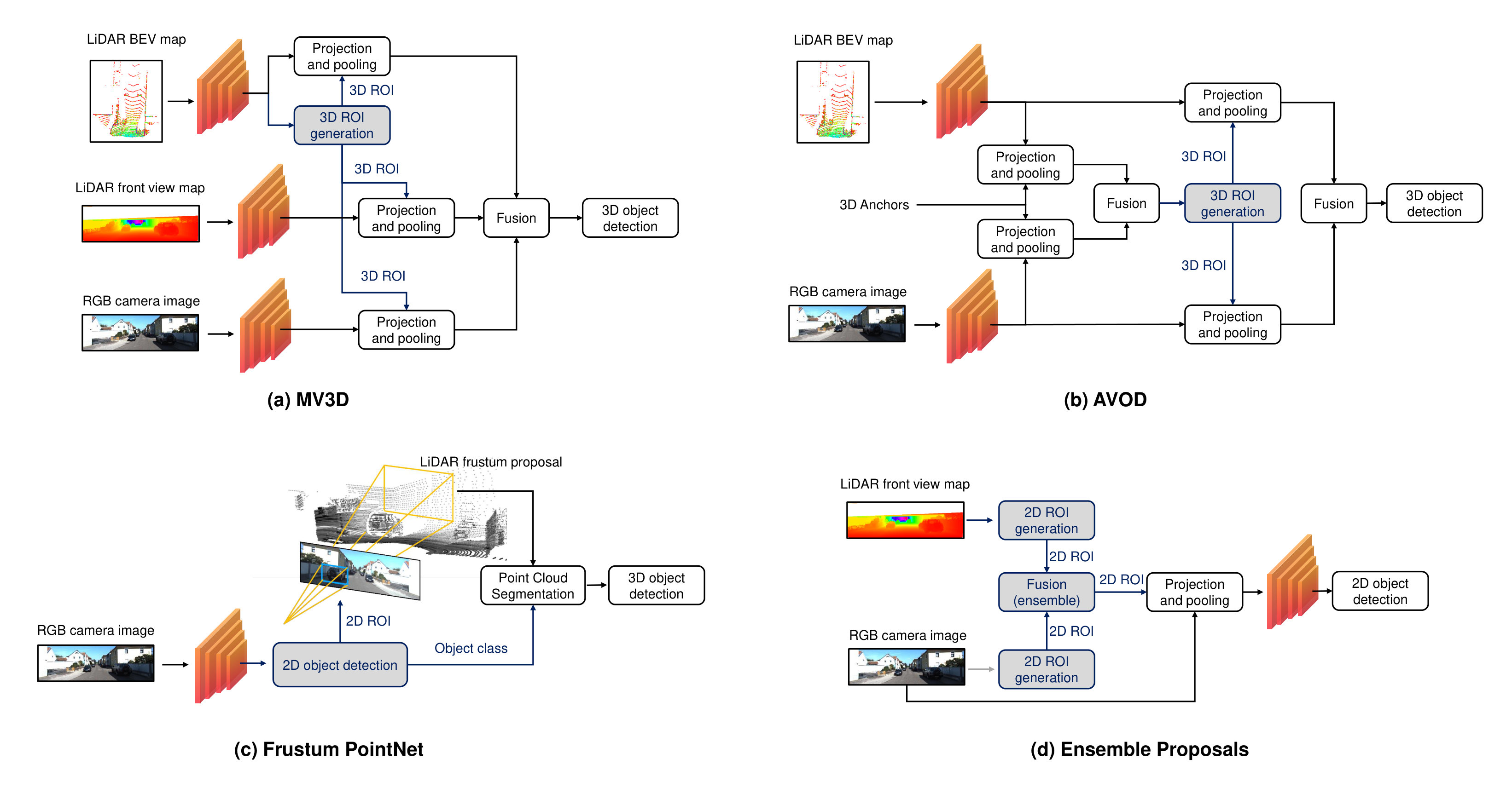 Figure 1
 Figure 2
 Figure 3
 Figure 4
 Figure 5
 Figure 6
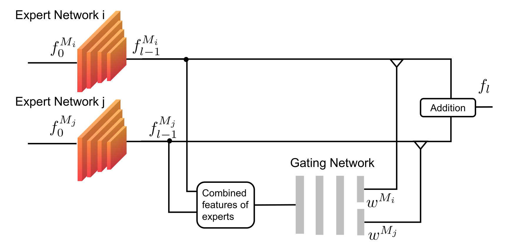 Figure 7
 Figure 8
 Figure 9
 Figure 10
 Figure 11
 Figure 12
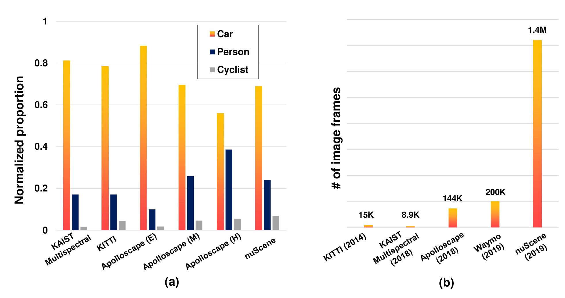 Figure 13
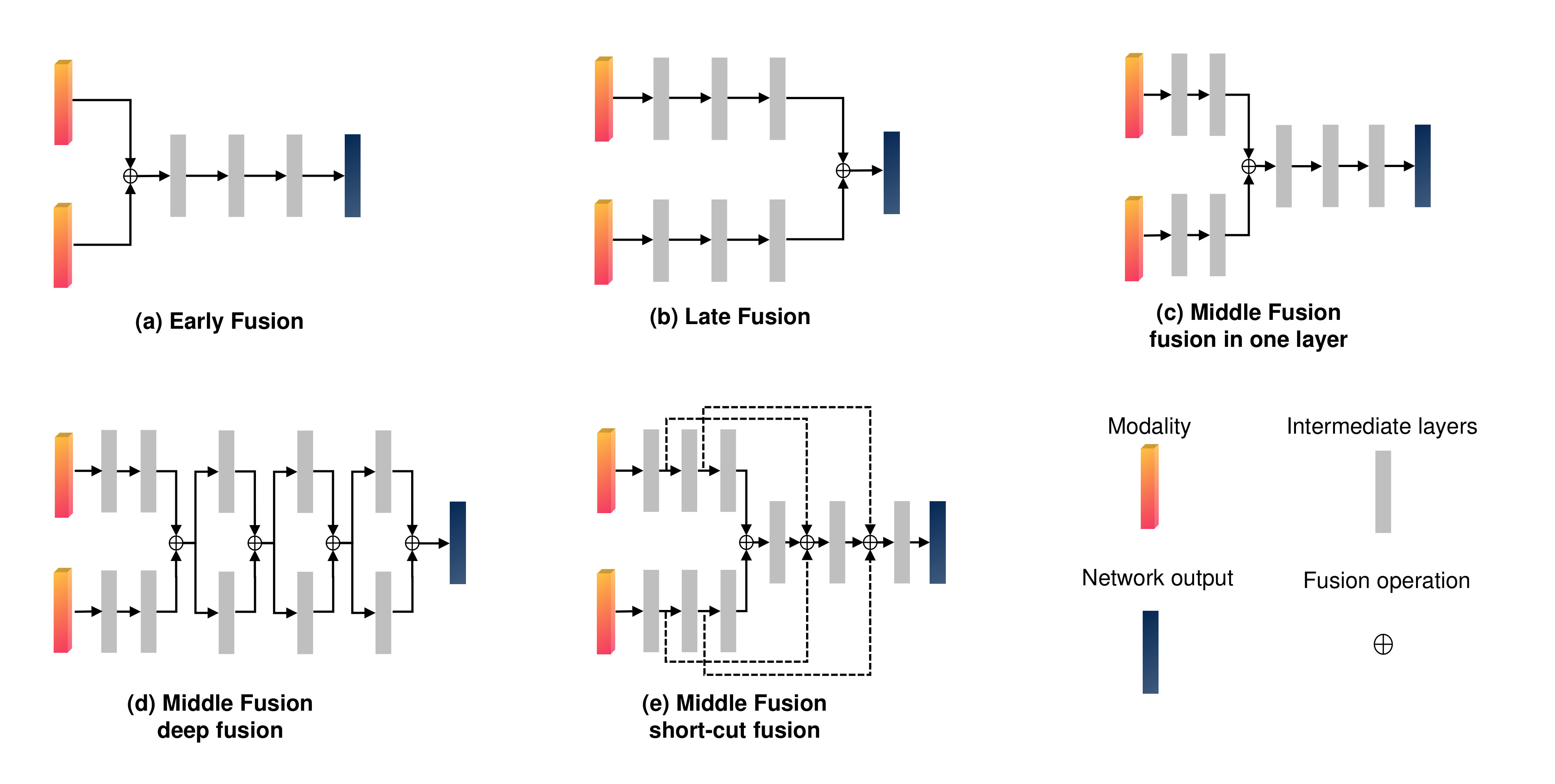 Figure 14
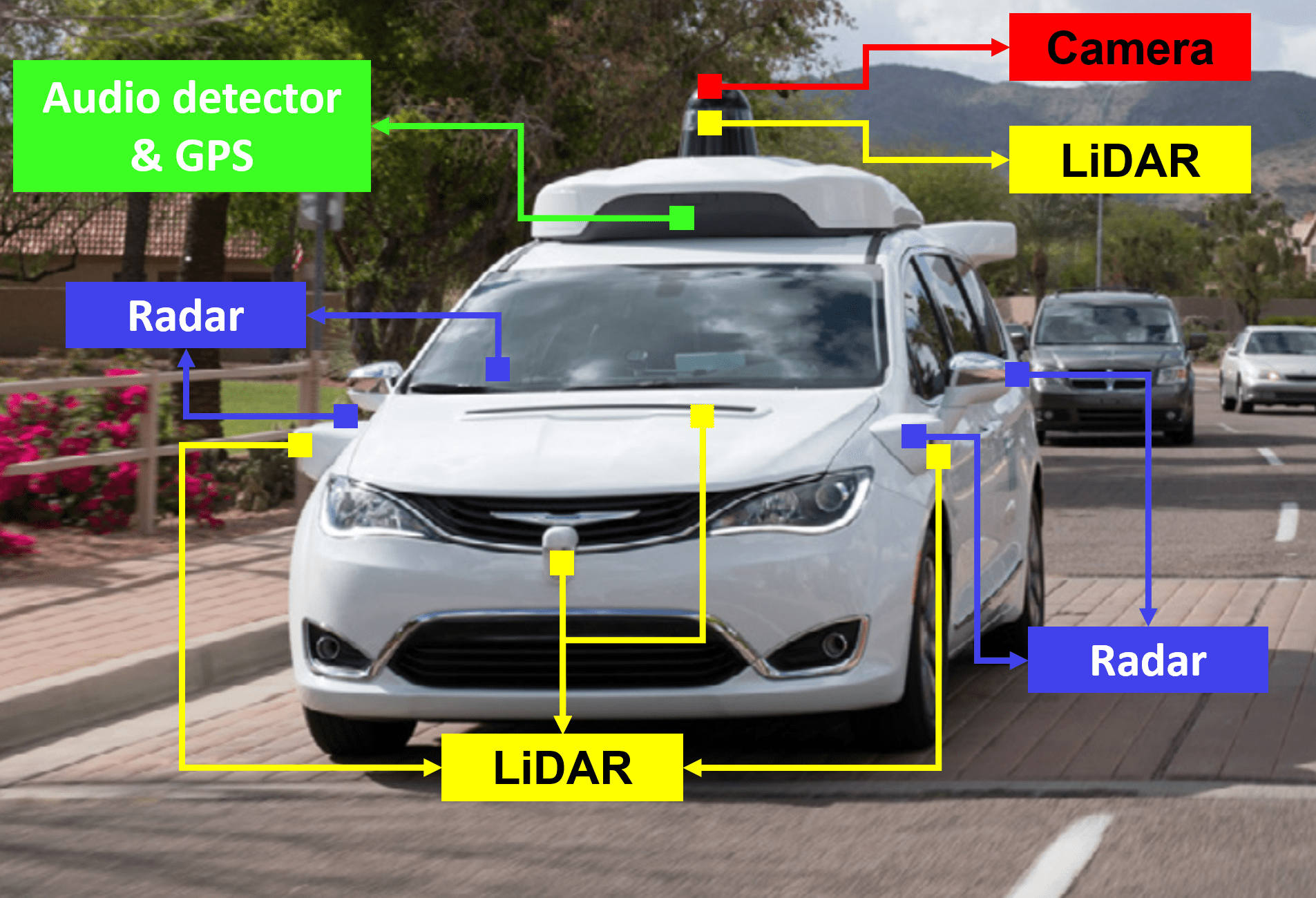 Figure 15
 Figure 16
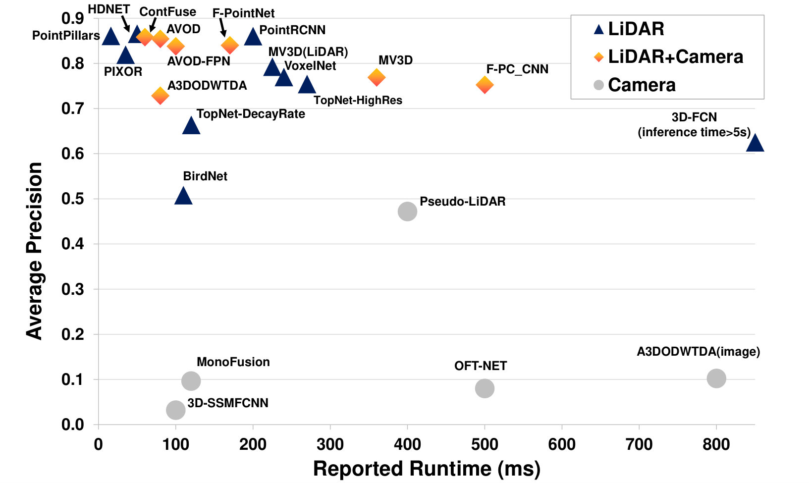 Figure 17
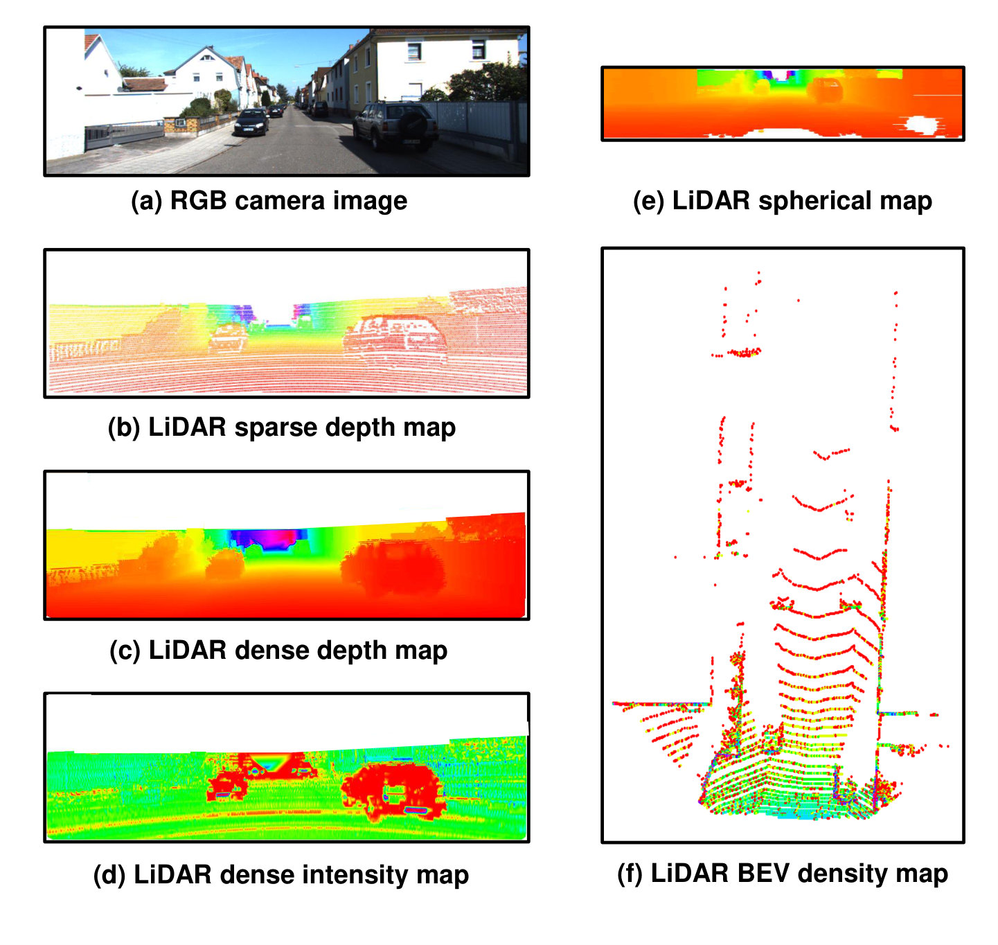 Figure 18
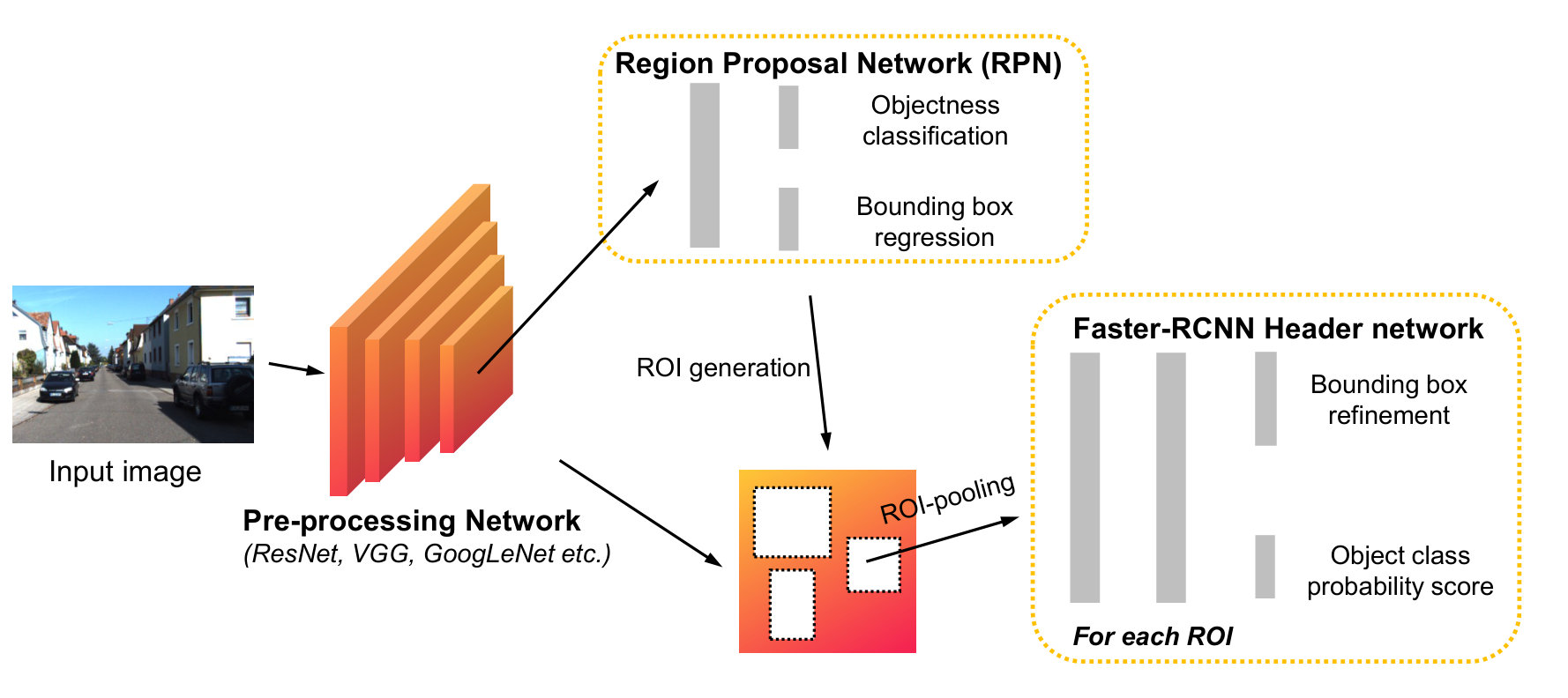 Figure 19
 Figure 20
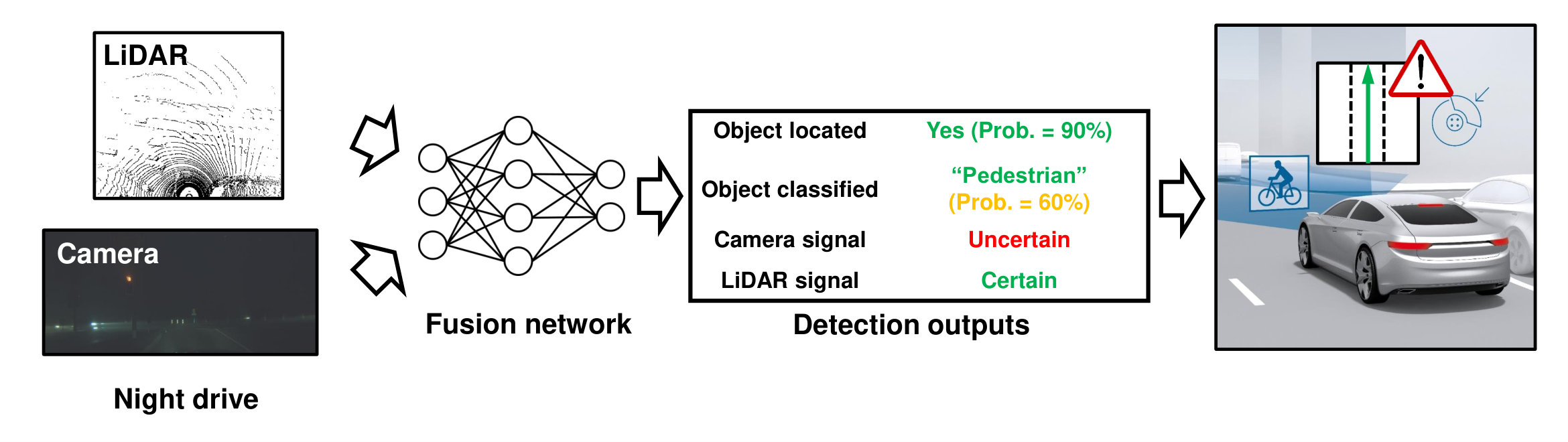 Figure 21
| \rowcolorlightgray!75 Topics | Challenges | Open Questions | |
|---|---|---|---|
| Multi-modal data preparation | Data diversity | • Relative small size of training dataset. • Limited driving scenarios and conditions, limited sensor variety, object class imbalance. | • Develop more realistic virtual datasets. • Finding optimal way to combine real- and virtual data. • Increasing labeling efficiency through cross-modal labeling, active learning, transfer learning, semi-supervised learning etc. Leveraging lifelong learning to update networks with continual data collection. |
| Data quality | • Labeling errors. • Spatial and temporal misalignment of different sensors. |
•
Teaching network robustness with erroneous and noisy labels.
•
Integrating prior knowledge in networks.
•
Developing methods (e.g. using deep learning) to automatically register sensors.
|
|
| Fusion methodology | “What to fuse” |
•
Too few sensing modalities are fused.
•
Lack of studies for different feature representations.
|
• Fusing multiple sensors with the same modality. • Fusing more sensing modalities, e.g. Radar, Ultrasonic, V2X communication. • Fusing with physical models and prior knowledge, also possible in the multi-task learning scheme. • Comparing different feature representation w.r.t informativeness and computational costs. |
| “How to fuse” |
•
Lack of uncertainty quantification for each sensor channel.
•
Too simple fusion operations.
|
•
Uncertainty estimation via e.g. Bayesian neural networks (BNN).
•
Propagating uncertainties to other modules, such as tracking and motion planning.
•
Anomaly detection by generative models.
•
Developing fusion operations that are suitable for network pruning and compression.
|
|
| “When to fuse” |
•
Fusion architecture is often designed by empirical results. No guideline for optimal fusion architecture design.
•
Lack of study for accuracy/speed or memory/robustness trade-offs.
|
•
Optimal fusion architecture search.
•
Incorporating requirements of computation time or memory as regularization term.
•
Using visual analytics tool to find optimal fusion architecture.
|
|
| Others | Evaluation metrics | • Current metrics focus on comparing networks’ accuracy. |
•
Metrics to quantify the networks’ robustness should be developed and adapted to multi-modal perception problems.
|
| More network architectures |
•
Current networks lack temporal cues and cannot guarantee prediction consistency over time.
•
They are designed mainly for modular autonomous driving.
|
•
Using Recurrent Neural Network (RNN) for sequential perception.
•
Multi-modal end-to-end learning or multi-modal direct-perception.
|
|
Peer Reviews
No public reviews on file for this paper yet. If you reviewed it on a platform where reviews are public (OpenReview, ICLR, NeurIPS, ICML), you can paste yours below so the community can read it here.
Code & Models
Videos
No videos yet. Explain this paper in a talk, walkthrough, or lecture? Add one.
Deep Multi-modal Object Detection and Semantic Segmentation for Autonomous Driving: Datasets, Methods, and Challenges
Di Feng, Christian Haase-Schütz, Lars Rosenbaum, Heinz Hertlein, Claudius Gläser, Fabian Timm, Werner Wiesbeck, Klaus Dietmayer ∗ Di Feng and Christian Haase-Schütz contributed equally to this work. Driver Assistance Systems and Automated Driving, Corporate Research, Robert Bosch GmbH, 71272 Renningen, Germany. Institute of Measurement, Control and Microtechnology, Ulm University, 89081 Ulm, Germany. Engineering Cognitive Systems, Automated Driving, Chassis Systems Control, Robert Bosch GmbH, 74232 Abstatt, Germany. Institute of Radio Frequency Engineering and Electronics, Karlsruhe Institute of Technology, 76131 Karlsruhe, Germany. † Corresponding author: [email protected]
Abstract
Recent advancements in perception for autonomous driving are driven by deep learning. In order to achieve robust and accurate scene understanding, autonomous vehicles are usually equipped with different sensors (e.g. cameras, LiDARs, Radars), and multiple sensing modalities can be fused to exploit their complementary properties. In this context, many methods have been proposed for deep multi-modal perception problems. However, there is no general guideline for network architecture design, and questions of “what to fuse”, “when to fuse”, and “how to fuse” remain open. This review paper attempts to systematically summarize methodologies and discuss challenges for deep multi-modal object detection and semantic segmentation in autonomous driving. To this end, we first provide an overview of on-board sensors on test vehicles, open datasets, and background information for object detection and semantic segmentation in autonomous driving research. We then summarize the fusion methodologies and discuss challenges and open questions. In the appendix, we provide tables that summarize topics and methods. We also provide an interactive online platform to navigate each reference: https://boschresearch.github.io/multimodalperception/.
Index Terms:
multi-modality, object detection, semantic segmentation, deep learning, autonomous driving
©2020 IEEE. Personal use of this material is permitted. Permission from IEEE must be obtained for all other uses, in any current or future media, including reprinting/republishing this material for advertising or promotional purposes, creating new collective works, for resale or redistribution to servers or lists, or reuse of any copyrighted component of this work in other works. DOI: 10.1109/TITS.2020.2972974.
I Introduction
Significant progress has been made in autonomous driving since the first successful demonstration in the 1980s [1] and the DARPA Urban Challenge in 2007 [2]. It offers high potential to decrease traffic congestion, improve road safety, and reduce carbon emissions [3]. However, developing reliable autonomous driving is still a very challenging task. This is because driverless cars are intelligent agents that need to perceive, predict, decide, plan, and execute their decisions in the real world, often in uncontrolled or complex environments, such as the urban areas shown in Fig. 1. A small error in the system can cause fatal accidents.
Perception systems in driverless cars need to be (1). accurate: they need to give precise information of driving environments; (2). robust: they should work properly in adverse weather, in situations that are not covered during training (open-set conditions), and when some sensors are degraded or even defective; and (3). real-time: especially when the cars are driving at high speed. Towards these goals, autonomous cars are usually equipped with multi-modal sensors (e.g. cameras, LiDARs, Radars), and different sensing modalities are fused so that their complementary properties are exploited (cf. Sec. II-A). Furthermore, deep learning has been very successful in computer vision. A deep neural network is a powerful tool for learning hierarchical feature representations given a large amount of data [5]. In this regard, many methods have been proposed that employ deep learning to fuse multi-modal sensors for scene understanding in autonomous driving. Fig. 2 shows some recently published methods and their performance on the KITTI dataset [6]. All methods with the highest performance are based on deep learning, and many methods that fuse camera and LiDAR information produce better performance than those using either LiDAR or camera alone. In this paper, we focus on two fundamental perception problems, namely, object detection and semantic segmentation. In the rest of this paper, we will call them deep multi-modal perception unless mentioned otherwise.
When developing methods for deep multi-modal object detection or semantic segmentation, it is important to consider the input data: Are there any multi-modal datasets available and how is the data labeled (cf. Tab. VII)? Do the datasets cover diverse driving scenarios (cf. Sec. VI-A1)? Is the data of high quality (cf. Sec. VI-A2)? Additionally, we need to answer several important questions on designing the neural network architecture: Which modalities should be combined via fusion, and how to represent and process them properly (“What to fuse” cf. Sec. VI-B1)? Which fusion operations and methods can be used (“How to fuse” cf. Sec. VI-B2)? Which stage of feature representation is optimal for fusion (“When to fuse” cf. Sec. VI-B2)?
I-A Related Works
Despite the fact that many methods have been proposed for deep multi-modal perception in autonomous driving, there is no published summary examining available multi-modal datasets, and there is no guideline for network architecture design. Yin et al. [7] summarize datasets for autonomous driving that were published between 2006 and 2016, including the datasets recorded with a single camera alone or multiple sensors. However, many new multi-modal datasets have been released since 2016, and it is worth summarizing them. Ramachandram et al. [8] provide an overview on deep multi-modal learning, and mention its applications in diverse research fields, such as robotic grasping and human action recognition. Janai et al. [9] conduct a comprehensive summary on computer vision problems for autonomous driving, such as scene flow and scene construction. Recently, Arnold et al. [10] survey the 3D object detection problem in autonomous driving. They summarize methods based on monocular images or point clouds, and briefly mention some works that fuse vision camera and LiDAR information.
I-B Contributions
To the best of our knowledge, there is no survey that focuses on deep multi-modal object detection (2D or 3D) and semantic segmentation for autonomous driving, which makes it difficult for beginners to enter this research field. Our review paper attempts to narrow this gap by conducting a summary of newly-published datasets (2013-2019), and fusion methodologies for deep multi-modal perception in autonomous driving, as well as by discussing the remaining challenges and open questions.
We first provide background information on multi-modal sensors, test vehicles, and modern deep learning approaches in object detection and semantic segmentation in Sec. II. We then summarize multi-modal datasets and perception problems in Sec. III and Sec. IV, respectively. Sec. V summarizes the fusion methodologies regarding “what to fuse”, “when to fuse” and “how to fuse”. Sec. VI discusses challenges and open questions when developing deep multi-modal perception systems in order to fulfill the requirements of “accuracy”, “robustness” and “real-time”, with a focus on data preparation and fusion methodology. We highlight the importance of data diversity, temporal and spatial alignment, and labeling efficiency for multi-modal data preparation. We also highlight the lack of research on fusing Radar signals, as well as the importance of developing fusion methodologies that tackle open dataset problems or increase network robustness. Sec. VII concludes this work. In addition, we provide an interactive online platform for navigating topics and methods for each reference. The platform can be found here: https://boschresearch.github.io/multimodalperception/.
II Background
This section provides the background information for deep multi-modal perception in autonomous driving. First, we briefly summarize typical automotive sensors, their sensing modalities, and some vehicles for test and research purposes. Next, we introduce deep object detection and semantic segmentation. Since deep learning has most-commonly been applied to image-based signals, here we mainly discuss image-based methods. We will introduce other methods that process LiDAR and Radar data in Sec. V-A. For a more comprehensive overview on object detection and semantic segmentation, we refer the interested reader to the review papers [11, 12]. For a complete review of computer vision problems in autonomous driving (e.g. optical flow, scene reconstruction, motion estimation), cf. [9].
II-A Sensing Modalities for Autonomous Driving
II-A1 Visual and Thermal Cameras
Images captured by visual and thermal cameras can provide detailed texture information of a vehicle’s surroundings. While visual cameras are sensitive to lighting and weather conditions, thermal cameras are more robust to daytime/nighttime changes as they detect infrared radiation that relates to heat from objects. However, both types of cameras however cannot directly provide depth information.
II-A2 LiDARs
LiDARs (Light Detection And Ranging) give accurate depth information of the surroundings in the form of 3D points. They measure reflections of laser beams which they emit with a certain frequency. LiDARs are robust to different lighting conditions, and less affected by various weather conditions such as fog and rain than visual cameras. However, typical LiDARs are inferior to cameras for object classification since they cannot capture the fine textures of objects, and their points become sparse with distant objects. Recently, flash LiDARs were developed which can produce detailed object information similar to camera images. Frequency Modulated Continuous Wave (FMCW) LiDARs can provide velocity information.
II-A3 Radars
Radars (Radio Detection And Ranging) emit radio waves to be reflected by an obstacle, measures the signal runtime, and estimates the object’s radial velocity by the Doppler effect. They are robust against various lighting and weather conditions, but classifying objects via Radars is very challenging due to their low resolution. Radars are often applied in adaptive cruise control (ACC) and traffic jam assistance systems [13].
II-A4 Ultrasonics
Ultrasonic sensors send out high-frequency sound waves to measure the distance to objects. They are typically applied for near-range object detection and in low speed scenarios, such as automated parking [13]. Due to the sensing properties, Ultrasonics are largely affected by air humidity, temperature, or dirt.
II-A5 GNSS and HD Maps
GNSS (Global Navigation Satellite Systems) provide accurate 3D object positions by a global satellite system and the receiver. Examples of GNSS are GPS, Galileo and GLONASS. First introduced to automotive as navigation tools in driver assistance functions [13], currently GNSS is also used together with HD Maps for path planning and ego-vehicle localization for autonomous vehicles.
II-A6 IMU and Odometers
Unlike sensors discussed above which capture information in the external environment (i.e. “exteroceptive sensors”), Inertial Measurement Units (IMU) and odometers provide vehicles’ internal information (i.e. “proprioceptive sensors”) [13]. IMU measure the vehicles’ accelerations and rotational rates, and odometers the odometry. They have been used in vehicle dynamic driving control systems since the 1980s. Together with the exteroceptive sensors, they are currently used for accurate localization in autonomous driving.
II-B Test Vehicle Setup
Equipped with multiple sensors introduced in Sec. II-A, many autonomous driving tests have been conducted. For example, the Tartan Racing Team developed an autonomous vehicle called “Boss” and won the DARPA Urban Challenge in 2007 (cf. Fig. 3) [2]. The vehicle was equipped with a camera and several Radars and LiDARs. Google (Waymo) has tested their driverless cars in more than US cities driving million miles on public roads (cf. Fig. 3) [14]; BMW has tested autonomous driving on highways around Munich since 2011 [15]; Daimler mounted a stereo camera, two mono cameras, and several Radars on a Mercedes Benz S-Class car to drive autonomously on the Bertha Benz memorial route in 2013 [16]. Our interactive online platform provides a detailed description for more autonomous driving tests, including Uber, Nvidia, GM Cruise, Baidu Apollo, as well as their sensor setup.
Besides driving demonstrations, real-world datasets are crucial for autonomous driving research. In this regard, several research projects use data vehicles with multi-modal sensors to build open datasets. These data vehicles are usually equipped with cameras, LiDARs and GPS/IMUs to collect images, 3D point clouds, and vehicle localization information. Sec. III provides an overview of multi-modal datasets in autonomous driving.
II-C Deep Object Detection
Object detection is the task of recognizing and localizing multiple objects in a scene. Objects are usually recognized by estimating a classification probability and localized with bounding boxes (cf. Fig. 1). Deep learning approaches have set the benchmark on many popular object detection datasets, such as PASCAL VOC [17] and COCO [18], and have been widely applied in autonomous driving, including detecting traffic lights [19, 20, 21, 22], road signs [23, 24, 25], people [26, 27, 28], or vehicles [29, 30, 31, 32, 33], to name a few. State-of-the-art deep object detection networks follow one of two approaches: the two-stage or the one-stage object detection pipelines. Here we focus on image-based detection.
II-C1 Two-stage Object Detection
In the first stage, several class-agnostic object candidates called regions of interest (ROI) or region proposals (RP) are extracted from a scene. Then, these candidates are verified, classified, and refined in terms of classification scores and locations. OverFeat [34] and R-CNN [35] are among pioneering works that employ deep learning for object detection. In these works, ROIs are first generated by the sliding window approach (OverFeat [34]) or selective search (R-CNN [35]) and then advanced into a regional CNN to extract features for object classification and bounding box regression. SPPnet [36] and Fast-RCNN [37] propose to obtain regional features directly from global feature maps by applying a larger CNN (e.g. VGG [38], ResNet [39], GoogLeNet [40]) on the whole image. Faster R-CNN [41] unifies the object detection pipeline and adopts the Region Proposal Network (RPN), a small fully-connected network, to slide over the high-level CNN feature maps for ROI generation (cf. Fig. 4). Following this line, R-FCN [42] proposes to replace fully-connected layers in an RPN with convolutional layers and builds a fully-convolutional object detector.
II-C2 One-stage Object Detection
This method aims to map the feature maps directly to bounding boxes and classification scores via a single-stage, unified CNN model. For example, MultiBox [43] predicts a binary mask from the entire input image via a CNN and infers bounding boxes at a later stage. YOLO [44] is a more complete unified detector which regresses the bounding boxes directly from the CNN model. SSD [45] handles objects with various sizes by regressing multiple feature maps of different resolution with small convolutional filters to predict multi-scale bounding boxes.
In general, two-stage object detectors like Faster-RCNN tend to achieve better detection accuracy due to the region proposal generation and refinement paradigm. This comes with the cost of higher inference time and more complex training. Conversely, one-stage object detectors are faster and easier to be optimized, yet under-perform compared to two-stage object detectors in terms of accuracy. Huang et al. [46] systematically evaluate the speed/accuracy trade-offs for several object detectors and backbone networks.
II-D Deep Semantic Segmentation
The target of semantic segmentation is to partition a scene into several meaningful parts, usually by labeling each pixel in the image with semantics (pixel-level semantic segmentation) or by simultaneously detecting objects and doing per-instance per-pixel labeling (instance-level semantic segmentation). Recently, panoptic segmentation [47] is proposed to unify pixel-level and instance-level semantic segmentation, and it starts to get more attentions for autonomous driving [48, 49, 50]. Though semantic segmentation was first introduced to process camera images, many methods have been proposed for segmenting LiDAR points as well (e.g. [51, 52, 53, 54, 55, 56]).
Many datasets have been published for semantic segmentation, such as Cityscape [57], KITTI [6], Toronto City [58], Mapillary Vistas [59], and ApolloScape [60]. These datasets advance the deep learning research for semantic segmentation in autonomous driving. For example, [61, 62, 54] focus on pixel-wise semantic segmentation for multiple classes including road, car, bicycle, column-pole, tree, sky, etc; [52] and [63] concentrate on road segmentation; and [64, 65, 51] deal with instance segmentation for various traffic participants.
Similar to object detection introduced in Sec. II-C, semantic segmentation can also be classified into two-stage and one-stage pipelines. In the two-stage pipeline, region proposals are first generated and then fine-tuned mainly for instance-level segmentation (e.g. R-CNN [66], SDS [67], Mask-RCNN [64]). A more common way for a semantic segmentation is the one-stage pipeline based on a Fully Convolutional Network (FCN) originally proposed by Long et al. [68]. In this work, the fully-connected layers in a CNN classifier for predicting classification scores are replaced with convolutional layers to produce coarse output maps. These maps are then up-sampled to dense pixel labels by backwards convolution (i.e. deconvolution). Kendall et al. [62] extend FCN by introducing an encoder-decoder CNN architecture. The encoder serves to produce hierarchical image representations with a CNN backbone such as VGG or ResNet (removing fully-connected layers). The decoder, conversely, restores these low-dimensional features back to original resolution by a set of upsampling and convolution layers. The restored feature maps are finally used for pixel-label prediction.
Global image information provides useful context cues for semantic segmentation. However, vanilla CNN structures only focus on local information with limited receptive fields. In this regard, many methods have been proposed to incorporate global information, such as dilated convolutions [69, 70], multi-scale prediction [71], as well as adding Conditional Random Fields (CRFs) as post-processing step [72].
Real-time performance is important in autonomous driving applications. However, most works only focus on segmentation accuracy. In this regard, Siam et al. [73] made a comparative study on the real-time performance among several semantic segmentation architectures, regarding the operations (GFLOPs) and the inference speed (fps).
III Multi-modal Datasets
Most deep multi-modal perception methods are based on supervised learning. Therefore, multi-modal datasets with labeled ground-truth are required for training such deep neural networks. In the following, we summarize several real-world datasets published since 2013, regarding sensor setups, recording conditions, dataset size and labels (cf. Tab. VII). Note that there exist some virtual multi-modal datasets generated from game engines. We will discuss them in Sec. VI-A1.
III-A Sensing Modalities
All reviewed datasets include RGB camera images. In addition, [74, 75, 6, 60, 76, 77, 78, 79, 80, 81, 82, 83, 84, 85, 86, 87, 88, 89] provide LiDAR point clouds, and [90, 91, 92] thermal images. The KAIST Multispectral Dataset [93] provides both thermal images and LiDAR data. Bus data is included additionally in [87]. Only the very recently nuScenes [89], Oxford Radar RobotCar [85] and Astyx HiRes2019 Datasets [94] provide Radar data.
III-B Recording Conditions
Even though the KITTI dataset [75] is widely used for autonomous driving research, the diversity of its recording conditions is relatively low: it is recorded in Karlsruhe - a mid-sized city in Germany, only during daytime and on sunny days. Other reviewed datasets such as [87, 88, 82, 89, 79, 60, 78] are recorded in more than one location. To increase the diversity of lighting conditions, [90, 91, 92, 60, 80, 84, 82, 86, 88, 89, 82, 81] collect data in both daytime and nighttime, and [93] considers various lighting conditions throughout the day, including sunrise, morning, afternoon, sunset, night, and dawn. The Oxford Dataset [74] and the Oxford Radar RobotCar Dataset [85] are collected by driving the car around the Oxford area during the whole year. It contains data under different weather conditions, such as heavy rain, night, direct sunlight and snow. Other datasets containing diverse weather conditions are [86, 88, 89, 60]. In [95], LiDAR is used as a reference sensor for generating ground-truth, hence we do not consider it a multi-modal dataset. However the diversity in the recording conditions is large, ranging from dawn to night, as well as reflections, rain and lens flare. The cross-season dataset [96] emphasizes the importance of changes throughout the year. However, it only provides camera images and labels for semantic segmentation. Similarly, the visual localization challenge and the corresponding benchmark [97] cover weather and season diversity (but no new multi-modal dataset is introduced). The recent Eurocity dataset [88] is the most diverse dataset we have reviewed. It is recorded in different cities from several European countries. All seasons are considered, as well as weather and daytime diversity. To date, the dataset is camera-only and other modalities (e.g. LiDARs) are announced.
III-C Dataset Size
The dataset size ranges from only 1,569 frames up to over 11 million frames. The largest dataset with ground-truth labels that we have reviewed is the nuScenes Dataset [89] with nearly 1,4M frames. Compared to the image datasets in the computer vision community, the multi-modal datasets are still relatively small. However, the dataset size has grown by two orders of magnitudes between 2014 and 2019 (cf. Fig. 5(b)).
III-D Labels
Most of the reviewed datasets provide ground-truth labels for 2D object detection and semantic segmentation tasks [90, 93, 75, 60, 91, 92, 88]. KITTI [75] also labels tracking, optical flow, visual odometry, and depth for various computer vision problems. BLV3D [80] provides labels for tracking, interaction and intention. Labels for 3D scene understanding are provided by [75, 60, 79, 80, 89, 81, 82, 83, 84].
Depending on the focus of a dataset, objects are labeled into different classes. For example, [90] only contains label for people, including distinguishable individuals (labeled as “Person”), non-distinguishable individuals (labeled as “People”), and cyclists; [60] classifies objects into five groups, and provides 25 fine-grained labels, such as truck, tricycle, traffic cone, and trash can. The Eurocity dataset [88] focuses on vulnerable road-users (mostly pedestrian). Instead of labeling objects, [77] provides a dataset for place categorization. Scenes are classified into forest, coast, residential area, urban area and indoor/outdoor parking lot. [78] provides vehicle speed and wheel angles for driving behavior predictions. The BLV3D dataset [80] provides unique labeling for interaction and intention.
The object classes are very imbalanced. Fig. 5(a) compares the percentage of car, person, and cyclist classes from four reviewed datasets. There are much more objects labeled as car than person or cyclist.
IV Deep Multi-modal Perception Problems for Autonomous Driving
In this section, we summarize deep multi-modal perception problems for autonomous driving based on sensing modalities and targets. An overview of the existing methods is shown in Tab. VII and Tab. VII. An accuracy and runtime comparison among several methods is shown in Tab. VII and Tab. VII.
IV-A Deep Multi-modal Object Detection
IV-A1 Sensing Modalities
Most existing works combine RGB images from visual cameras with 3D LiDAR point clouds [98, 99, 100, 101, 102, 103, 104, 105, 106, 107, 108, 109, 110, 111, 112, 113, 114, 115, 116]. Some other works focus on fusing the RGB images from visual cameras with images from thermal cameras [117, 118, 119, 91]. Furthermore, Mees et al. [120] employ a Kinect RGB-D camera to fuse RGB images and depth images; Schneider et al. [61] generate depth images from a stereo camera and combine them with RGB images; Yang et al. [121] and Cascas et al. [122] leverage HD maps to provide prior knowledge of the road topology.
IV-A2 2D or 3D Detection
Many works [99, 100, 106, 108, 109, 61, 120, 117, 91, 118, 101, 119, 123, 111] deal with the 2D object detection problem on the front-view 2D image plane. Compared to 2D detection, 3D detection is more challenging since the object’s distance to the ego-vehicle needs to be estimated. Therefore, accurate depth information provided by LiDAR sensors is highly beneficial. In this regard, some papers including [98, 102, 103, 104, 105, 107, 115, 113] combine RGB camera images and LiDAR point clouds for 3D object detection. In addition, Liang et al. [116] propose a multi-task learning network to aid 3D object detection. The auxiliary tasks include camera depth completion, ground plane estimation, and 2D object detection. How to represent the modalities properly is discussed in section V-A.
IV-A3 What to detect
Complex driving scenarios often contain different types of road users. Among them, cars, cyclists, and pedestrians are highly relevant to autonomous driving. In this regard, [98, 99, 106, 108, 110] employ multi-modal neural networks for car detection; [101, 108, 109, 120, 117, 118, 119] focus on detecting non-motorized road users (pedestrians or cyclists); [100, 102, 103, 104, 105, 61, 91, 111, 115, 116] detect both.
IV-B Deep Multi-modal Semantic Segmentation
Compared to the object detection problem summarized in Sec. IV-A, there are fewer works on multi-modal semantic segmentation: [119, 92, 124] employ RGB and thermal images, [61] fuses RGB images and depth images from a stereo camera, [125, 126, 127] combine RGB, thermal, and depth images for semantic segmentation in diverse environments such as forests, [123] fuses RGB images and LiDAR point clouds for off-road terrain segmentation and [128, 129, 130, 131, 132] for road segmentation. Apart from the above-mentioned works for semantic segmentation on the 2D image plane, [133, 125] deal with 3D segmentation on LiDAR points.
V Methodology
When designing a deep neural network for multi-modal perception, three questions need to be addressed - What to fuse: what sensing modalities should be fused, and how to represent and process them in an appropriate way; How to fuse: what fusion operations should be utilized; When to fuse: at which stage of feature representation in a neural network should the sensing modalities be combined. In this section, we summarize existing methodologies based on these three aspects.
V-A What to Fuse
LiDARs and cameras (visual cameras, thermal cameras) are the most common sensors for multi-modal perception in the literature. While the interest in processing Radar signals via deep learning is growing, only a few papers discuss deep multi-modal perception with Radar for autonomous driving (e.g. [134]). Therefore, we focus on several ways to represent and process LiDAR point clouds and camera images separately, and discuss how to combine them together. In addition, we briefly summarize Radar perception using deep learning.
V-A1 LiDAR Point Clouds
LiDAR point clouds provide both depth and reflectance information of the environment. The depth information of a point can be encoded by its Cartesian coordinates , distance , density, or HHA features (Horizontal disparity, Height, Angle) [66], or any other 3D coordinate system. The reflectance information is given by intensity.
There are mainly three ways to process point clouds. One way is by discretizing the 3D space into 3D voxels and assigning the points to the voxels (e.g. [135, 113, 29, 136, 137]). In this way, the rich 3D shape information of the driving environment can be preserved. However, this method results in many empty voxels as the LiDAR points are usually sparse and irregular. Processing the sparse data via clustering (e.g. [100, 106, 107, 108]) or 3D CNN (e.g. [29, 136]) is usually very time-consuming and infeasible for online autonomous driving. Zhou et al. [135] propose a voxel feature encoding (VFE) layer to process the LiDAR points efficiently for 3D object detection. They report an inference time of on the KITTI dataset. Yan et al. [138] add several sparse convolutional layers after the VFE to convert the sparse voxel data into 2D images, and then perform 3D object detection on them. Unlike the common convolution operation, the sparse convolution only computes on the locations associated with input points. In this way, they save a lot of computational cost, achieving an inference time of only .
The second way is to directly learn over 3D LiDAR points in continuous vector space without voxelization. PointNet [139] and its improved version PointNet++ [140] propose to predict individual features for each point and aggregate the features from several points via max pooling. This method was firstly introduced in 3D object recognition and later extended by Qi et al. [105], Xu et al. [104] and Shin et al. [141] to 3D object detection in combination with RGB images. Furthermore, Wang et al. [142] propose a new learnable operator called Parametric Continuous Convolution to aggregate points via a weighted sum, and Li et al. [143] propose to learn a transformation before applying transformed point cloud features into standard CNN. They are tested in semantic segmentation or LiDAR motion estimation tasks.
A third way to represent 3D point clouds is by projecting them onto 2D grid-based feature maps so that they can be processed via 2D convolutional layers. In the following, we distinguish among spherical map, camera-plane map (CPM), as well as bird’s eye view (BEV) map. Fig. 6 illustrates different LiDAR representations in 2D.
A spherical map is obtained by projecting each 3D point onto a sphere, characterized by azimuth and zenith angles. It has the advantage of representing each 3D point in a dense and compact way, making it a suitable representation for point cloud segmentation (e.g. [51]). However, the size of the representation can be different from camera images. Therefore, it is difficult to fuse them at an early stage. A CPM can be produced by projecting the 3D points into the camera coordinate system, provided the calibration matrix. A CPM can be directly fused with camera images, as their sizes are the same. However, this representation leaves many pixels empty. Therefore, many methods have been proposed to up-sample such a sparse feature map, e.g. mean average [111], nearest neighbors [144], or bilateral filter [145]. Compared to the above-mentioned feature maps which encode LiDAR information in the front-view, a BEV map avoids occlusion problems because objects occupy different space in the map. In addition, the BEV preserves the objects’ length and width, and directly provides the objects’ positions on the ground plane, making the localization task easier. Therefore, the BEV map is widely applied to 3D environment perception. For example, Chen et al. [98] encode point clouds by height, density and intensity maps in BEV. The height maps are obtained by dividing the point clouds into several slices. The density maps are calculated as the number of points within a grid cell, normalized by the number of channels. The intensity maps directly represent the reflectance measured by the LiDAR on a grid. Lang et al. [146] argue that the hard-coded features for BEV representation may not be optimal. They propose to learn features in each column of the LiDAR BEV representation via PointNet [139], and feed these learnable feature maps to standard 2D convolution layers.
V-A2 Camera Images
Most methods in the literature employ RGB images from visual cameras or one type of infrared images from thermal cameras (near-infrared, mid-infrared, far-infrared). Besides, some works extract additional sensing information, such as optical flow [120], depth [61, 126, 125], or other multi-spectral images [125, 91].
Camera images provide rich texture information of the driving surroundings. However, objects can be occluded and the scale of a single object can vary significantly in the camera image plane. For 3D environment inference, the bird’s eye view that is commonly used for LiDAR point clouds might be a better representation. Roddick et al. [147] propose a Orthographic Feature Transform (OFT) algorithm to project the RGB image features onto the BEV plane. The BEV feature maps are further processed for 3D object detection from monocular camera images. Lv et al. [130] project each image pixel with the corresponding LiDAR point onto the BEV plane and fuse the multi-modal features for road segmentation. Wang et al. [148] and their successive work [149] propose to convert RGB images into pseudo-lidar representation by estimating the image depth, and then use state-of-the-art BEV LiDAR detector to significantly improve the detection performance.
V-A3 Processing LiDAR Points and Camera Images in Deep Multi-modal Perception
Tab. VII and Tab. VII summarize existing methods to process sensors’ signals for deep multi-modal perception, mainly LiDAR points and camera images. From the tables we have three observations: (1). Most works propose to fuse LiDAR and camera features extracted from 2D convolution neural networks. To do this, they project LiDAR points on the 2D plane and process the feature maps through 2D convolutions. Only a few works extract LiDAR features by PointNet (e.g. [104, 105, 128]) or 3D convolutions (e.g. [123]); (2). Several works on multi-modal object detection cluster and segment 3D LiDAR points to generate 3D region proposals (e.g. [100, 106, 108]). Still, they use a LiDAR 2D representation to extract features for fusion; (3). Several works project LiDAR points on the camera-plane or RGB camera images on the LiDAR BEV plane (e.g. [130, 131, 150]) in order to align the features from different sensors, whereas many works propose to fuse LiDAR BEV features directly with RGB camera images (e.g. [98, 103]). This indicates that the networks implicitly learn to align features of different viewpoints. Therefore, a well-calibrated sensor setup with accurate spatial and temporal alignment is the prerequisite for accurate multi-modal perception, as will be discussed in Sec. VI-A2.
V-A4 Radar Signals
Radars provide rich environment information based on received amplitudes, ranges, and the Doppler spectrum. The Radar data can be represented by 2D feature maps and processed by convolutional neural networks. For example, Lombacher et al. employ Radar grid maps made by accumulating Radar data over several time-stamps [151] for static object classification [152] and semantic segmentation [153] in autonomous driving. Visentin et al. show that CNNs can be employed for object classification in a post-processed range-velocity map [154]. Kim et al. [155] use a series of Radar range-velocity images and convolutional recurrent neural networks for moving objects classification. Moeness et al. [156] feed spectrogram from Time Frequency signals as 2D images into a stacked auto-encoders to extract high-level Radar features for human motion recognition. The Radar data can also be represented directly as “point clouds” and processed by PointNet++ [140] for dynamic object segmentation [157]. Besides, Woehler et al. [158] encode features from a cluster of Radar points for dynamic object classification. Chadwick et al. [134] first project Radar points on the camera plane to build Radar range-velocity images, and then combine with camera images for distant vehicle detection.
V-B How to Fuse
This section summarizes typical fusion operations in a deep neural network. For simplicity we restrict our discussion to two sensing modalities, though more still apply. Denote and as two different modalities, and and their feature maps in the layer of the neural network. Also denote as a mathematical description of the feature transformation applied in layer of the neural network.
V-B1 Addition or Average Mean
This join operation adds the feature maps element-wise, i.e. , or calculates the average mean of the feature maps.
V-B2 Concatenation
Combines feature maps by . The feature maps are usually stacked along their depth before they are advanced to a convolution layer. For a fully connected layer, these features are usually flattened into vectors and concatenated along the rows of the feature maps.
V-B3 Ensemble
This operation ensembles feature maps from different sensing modalities via . As will be introduced in the following sections (Sec. V-C4 and Sec. V-C5), ensembles are often used to fuse ROIs in object detection networks.
V-B4 Mixture of Experts
The above-mentioned fusion operations do not consider the informativeness of a sensing modality (e.g. at night time RGB camera images bring less information than LiDAR points). These operations are applied, hoping that the network can implicitly learn to weight the feature maps. In contrast, the Mixture of Experts (MoE) approach explicitly models the weight of a feature map. It is first introduced in [159] for neural networks and then extended in [160, 120, 126]. As Fig. 7 illustrates, the feature map of a sensing modality is processed by its domain-specific network called “expert”. Afterwards, the outputs of multiple expert networks are averaged with the weights predicted by a gating network which takes the combined features output by the expert networks as inputs via a simple fusion operation such as concatenation:
[TABLE]
V-C When to Fuse
Deep neural networks represent features hierarchically and offer a wide range of choices to combine sensing modalities at early, middle, or late stages (Fig. 8). In the sequel, we discuss the early, middle, and late fusions in detail. For each fusion scheme, we first give mathematical descriptions using the same notations as in Sec. V-B, and then discuss their properties. Note that there exists some works that fuse features from the early stage till late stages in deep neural networks (e.g. [161]). For simplicity, we categorize this fusion scheme as “middle fusion”. Compared to the semantic segmentation where multi-modal features are fused at different stages in FCN, there exist more diverse network architectures and more fusion variants in object detection. Therefore, we additionally summarize the fusion methods specifically for the object detection problem. Finally, we discuss the relationship between the fusion operation and the fusion scheme.
Note that we do not find conclusive evidence from the methods we have reviewed that one fusion method is better than the others. The performance is highly dependent on sensing modalities, data, and network architectures.
V-C1 Early Fusion
This method fuses the raw or pre-processed sensor data. Let us define as a fusion operation introduced in Sec. V-B. For a network that has layers, an early fusion scheme can be described as:
[TABLE]
with . Early fusion has several pros and cons. First, the network learns the joint features of multiple modalities at an early stage, fully exploiting the information of the raw data. Second, early fusion has low computation requirements and a low memory budget as it jointly processes the multiple sensing modalities. This comes with the cost of model inflexibility. As an example, when an input is replaced with a new sensing modality or the input channels are extended, the early fused network needs to be retrained completely. Third, early fusion is sensitive to spatial-temporal data misalignment among sensors which are caused by calibration error, different sampling rate, and sensor defect.
V-C2 Late Fusion
This fusion scheme combines decision outputs of each domain specific network of a sensing modality. It can be described as:
[TABLE]
Late fusion has high flexibility and modularity. When a new sensing modality is introduced, only its domain specific network needs to be trained, without affecting other networks. However, it suffers from high computation cost and memory requirements. In addition, it discards rich intermediate features which may be highly beneficial when being fused.
V-C3 Middle Fusion
Middle fusion is the compromise of early and late fusion: It combines the feature representations from different sensing modalities at intermediate layers. This enables the network to learn cross modalities with different feature representations and at different depths. Define as the layer from which intermediate features begin to be fused. The middle fusion can be executed at this layer only once:
[TABLE]
Alternatively, they can be fused hierarchically, such as by deep fusion [162, 98]:
[TABLE]
or “short-cut fusion” [92]:
[TABLE]
Although the middle fusion approach is highly flexible, it is not easy to find the “optimal” way to fuse intermediate layers given a specific network architecture. We will discuss this challenge in detail in Sec. VI-B3.
V-C4 Fusion in Object Detection Networks
Modern multi-modal object detection networks usually follow either the two-stage pipeline (RCNN [35], Fast-RCNN [37], Faster-RCNN [41]) or the one-stage pipeline (YOLO [44] and SSD [45]), as explained in detail in Sec. II-C. This offers a variety of alternatives for network fusion. For instance, the sensing modalities can be fused to generate regional proposals for a two-stage object detector. The regional multi-modal features for each proposal can be fused as well. Ku et al. [103] propose AVOD, an object detection network that fuses RGB images and LiDAR BEV images both in the region proposal network and the header network. Kim et al. [109] ensemble the region proposals that are produced by LiDAR depth images and RGB images separately. The joint region proposals are then fed to a convolutional network for final object detection. Chen et al. [98] use LiDAR BEV maps to generate region proposals. For each ROI, the regional features from the LiDAR BEV maps are fused with those from the LiDAR front-view maps as well as camera images via deep fusion. Compared to object detections from LiDAR point clouds, camera images have been well investigated with larger labeled dataset and better 2D detection performance. Therefore, it is straightforward to exploit the predictions from well-trained image detectors when doing camera-LiDAR fusion. In this regard, [105, 107, 104] propose to utilize a pre-trained image detector to produce 2D bounding boxes, which build frustums in LiDAR point clouds. Then, they use these point clouds within the frustums for 3D object detection. Fig. 9 shows some exemplary fusion architectures for two-stage object detection networks. Tab. VII summarizes the methodologies for multi-modal object detection.
V-C5 Fusion Operation and Fusion Scheme
Based on the papers that we have reviewed, feature concatenation is the most common operation, especially at early and middle stages. Element-wise average mean and addition operations are additionally used for middle fusion. Ensemble and Mixture of Experts are often used for middle to decision level fusion.
The reference list from the paper itself. Each links out to its DOI / PubMed record.
- 1[1] E. D. Dickmanns and B. D. Mysliwetz, “Recursive 3-d road and relative ego-state recognition,” IEEE Trans. Pattern Anal. Mach. Intell. , no. 2, pp. 199–213, 1992.
- 2[2] C. Urmson et al. , “Autonomous driving in urban environments: Boss and the urban challenge,” J. Field Robotics , vol. 25, no. 8, pp. 425–466, 2008.
- 3[3] R. Berger, “Autonomous driving,” Think Act , 2014. [Online]. Available: http://www.rolandberger.ch/media/pdf/Roland_Berger_TAB Autonomous Drivingfinal 20141211
- 4[4] G. Neuhold, T. Ollmann, S. R. Bulò, and P. Kontschieder, “The Mapillary Vistas dataset for semantic understanding of street scenes,” in Proc. IEEE Conf. Computer Vision , Oct. 2017, pp. 5000–5009.
- 5[5] Y. Le Cun, Y. Bengio, and G. Hinton, “Deep learning,” Nature , vol. 521, no. 7553, p. 436, 2015.
- 6[6] A. Geiger, P. Lenz, and R. Urtasun, “Are we ready for autonomous driving? the KITTI vision benchmark suite,” in Proc. IEEE Conf. Computer Vision and Pattern Recognition , 2012.
- 7[7] H. Yin and C. Berger, “When to use what data set for your self-driving car algorithm: An overview of publicly available driving datasets,” in IEEE 20th Int. Conf. Intelligent Transportation Systems , 2017, pp. 1–8.
- 8[8] D. Ramachandram and G. W. Taylor, “Deep multimodal learning: A survey on recent advances and trends,” IEEE Signal Process. Mag. , vol. 34, no. 6, pp. 96–108, 2017.
