Integrable Floquet Hamiltonian for a Periodically Tilted 1D Gas
Andrea Colcelli, Giuseppe Mussardo, German Sierra, Andrea Trombettoni

TL;DR
This paper demonstrates that a periodically driven Lieb--Liniger model with a linear potential remains integrable, allowing exact solutions for its quasi-energies and insights into its dynamics, with potential experimental realizations.
Contribution
It shows that the Floquet Hamiltonian of an integrable 1D Bose gas under periodic linear tilt is itself integrable, enabling exact Bethe ansatz solutions.
Findings
Floquet Hamiltonian remains integrable under periodic linear tilt.
Quasi-energies can be exactly determined using Bethe ansatz.
Proposes an experimental setup with shaken ring potential.
Abstract
An integrable model subjected to a periodic driving gives rise generally to a non-integrable Floquet Hamiltonian. Here we show that the Floquet Hamiltonian of the integrable Lieb--Liniger model in presence of a linear potential with a periodic time--dependent strength is instead integrable and its quasi-energies can be determined using the Bethe ansatz approach. We discuss various aspects of the dynamics of the system at stroboscopic times and we also propose a possible experimental realisation of the periodically driven tilting in terms of a shaken rotated ring potential.
Click any figure to enlarge with its caption.
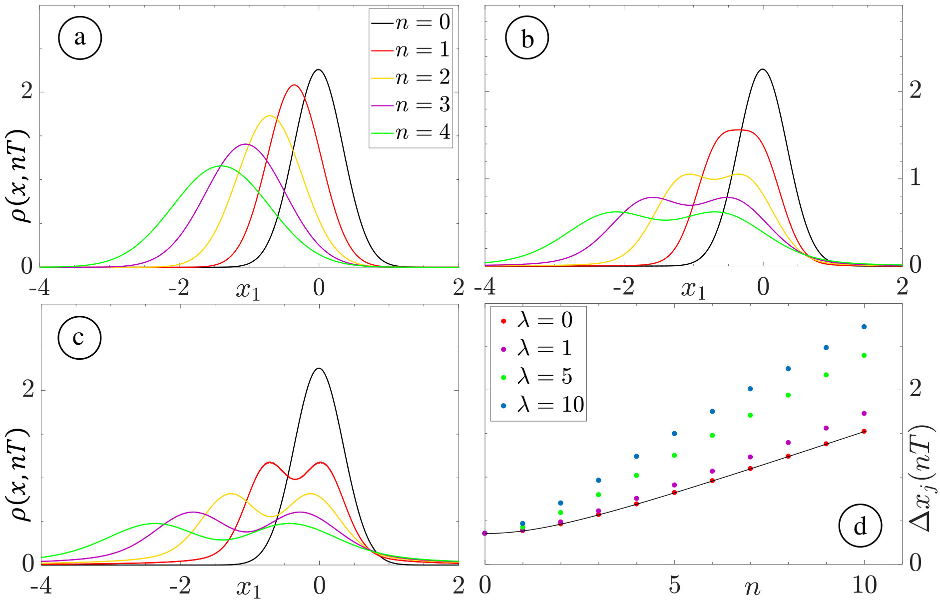 Figure 1
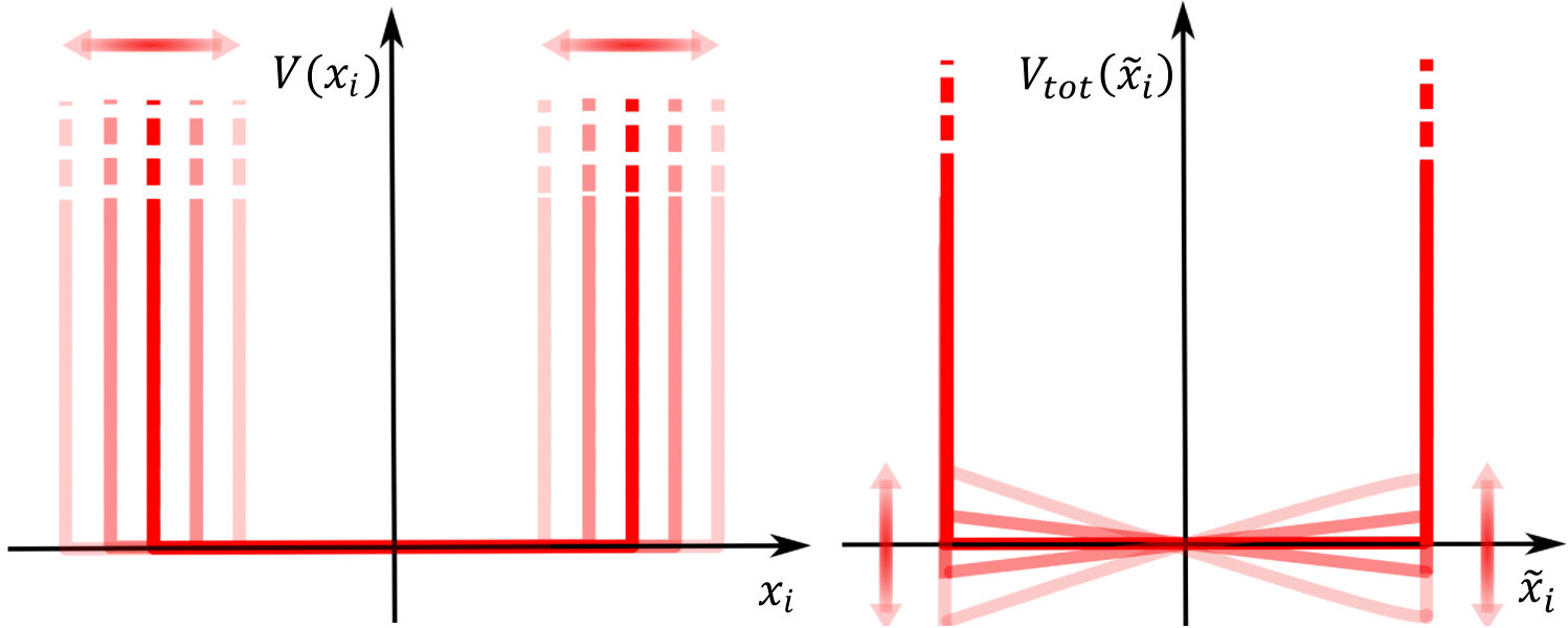 Figure 2
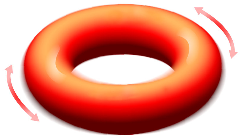 Figure 3
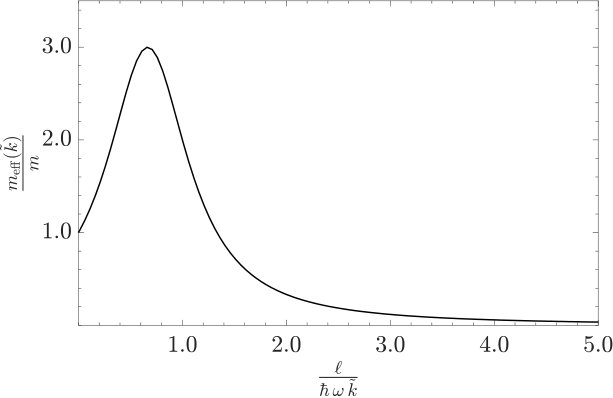 Figure 4
Peer Reviews
No public reviews on file for this paper yet. If you reviewed it on a platform where reviews are public (OpenReview, ICLR, NeurIPS, ICML), you can paste yours below so the community can read it here.
Videos
No videos yet. Explain this paper in a talk, walkthrough, or lecture? Add one.
Integrable Floquet Hamiltonian for a Periodically Tilted Gas
A. Colcelli
SISSA and INFN, Sezione di Trieste, Via Bonomea 265, I-34136 Trieste, Italy
G. Mussardo
SISSA and INFN, Sezione di Trieste, Via Bonomea 265, I-34136 Trieste, Italy
G. Sierra
Instituto de Física Teórica, UAM/CSIC, Universidad Autónoma de Madrid, Madrid, Spain
A. Trombettoni
CNR-IOM DEMOCRITOS Simulation Center, Via Bonomea 265, I-34136 Trieste, Italy
SISSA and INFN, Sezione di Trieste, Via Bonomea 265, I-34136 Trieste, Italy
Abstract
An integrable model subjected to a periodic driving gives rise generally to a non-integrable Floquet Hamiltonian. Here we show that the Floquet Hamiltonian of the integrable Lieb–Liniger model in presence of a linear potential with a periodic time–dependent strength is instead integrable and its quasi-energies can be determined using the Bethe ansatz approach. We discuss various aspects of the dynamics of the system at stroboscopic times and we also propose a possible experimental realisation of the periodically driven tilting in terms of a shaken rotated ring potential.
I Introduction
Floquet theory is a powerful tool to study differential equations whose coefficients are time–periodic functions Floquet883 and, for this reason, it is widely used in Quantum Mechanics in presence of a time–periodic Hamiltonian Shirley65 ; Grifoni98 . If the system is initially in state and subjected to a periodic driving, then the Floquet Hamiltonian is the operator that formally gives the state of the system at multiples of the period :
[TABLE]
depends on the parameters of the original driven Hamiltonian, , and of course on the time–dependent perturbation. The eigenvalues of the Floquet Hamiltonian are the quasi-energies . Often referred as Floquet engineering Eckardt2017 ; Oka18 , time–periodic driving allows to construct interesting effective with novel physical properties as, for instance, dynamic localization effects Dunlap1986 , suppression of inter–well tunneling in a Bose condensate subjected to a strongly driven optical lattice Creffield2003 ; Eckardt2005 ; Lignier2007 ; Kierig2008 ; Eckardt2009 ; Sierra2015 (see Eckardt2017 for more references), topological Floquet phases Kitagawa2010 ; Lindner2011 , time crystals Wilczek2013 ; Watanabe2015 ; Choi2017 ; Zhang2017 ; Russomanno2017 ; Yao2017 ; SachaZak2018 ; Sacha2018 , dynamics in driven systems Russomanno2012 ; Goldman2014 ; Holthaus2016 and Floquet prethermalization Weidinger17 ; Herrmann18 .
Within this framework, a natural question is whether one can have an integrable non-trivial Floquet Hamiltonian perturbing an interacting model with a time–periodic perturbation. Despite exactly solvable time–dependent Hamiltonians can be constructed Yuzbashyan18 ; Sinitsyn18 , the problem of finding an integrable Floquet Hamiltonian from undriven interacting (possibly integrable) Hamiltonian is in general a challenging one. Our scope is to present explicitly an interacting many-body system whose Floquet Hamiltonian is indeed integrable and therefore exactly solvable by means of integrability techniques Korepin1993 ; Mussardo10 . This implies, in particular, that we can have access to the exact spectrum of the quasi-energies and also to the wavefunctions of the system at stroboscopic times (multiples of the period of the driving). It is useful to stress that one of the difficulties in identifying integrable Floquet Hamiltonians is that the integrability of these Hamiltonians is not at all guaranteed by the integrability of the original time-independent undriven model (see, for instance, Komnik16 where starting from the original BCS model the corresponding BCS gap equation in presence of a periodic driving is derived and solved numerically).
The original time–independent system that we consider in the following is the Lieb–Liniger (LL) model which describes the -contact repulsion between bosons in one dimension LiebLiniger1963 : this model is exactly solvable using Bethe ansatz techniques LiebLiniger1963 ; Yang1969 , and routinely used to describe (quasi) one–dimensional bosonic gases realized in ultracold atoms experiments (see the reviews Yurovsky2008 ; Bouchoule2009 ; Cazalilla2011 ). Interestingly enough, this quantum model remains exactly solvable also when it is perturbed by an external time–periodic potential linear in the coordinates of the particles, as it happens for its classical counterpart given by the non–linear Schrödinger equation which remains solvable also in presence of an external linear time–dependent potential Chen ; Ablowitz2004 . Our system is then the quantum analog of a classical mechanics problem consisting of a body (subjected to the gravity force) put on a slide which changes periodically its slope by rotating around a pin posed at the origin. Before addressing the many-body Floquet Hamiltonian of the LL model, it is interesting to discuss preliminarily two instructive cases of 1D systems subjected to time–periodic linear potential: (a) the case of one particle and (b) the case of two interacting particles.
II One particle
The Schrödinger equation for a particle of mass in a linear time–periodic potential in reads
[TABLE]
where . Eq. (2) has been studied and solved in several different ways Berry1978 ; Rau1996 ; Guedes2001 ; Feng2001 . Here we derive and discuss the results coming from Floquet theory in order to study the behaviour of the system at stroboscopic times, i.e. at multiples of the period . To this aim, we perform a gauge transformation on the wavefunction
[TABLE]
where , with and to be determined. Substituting (3) into (2), we find that if and , then satisfies the Schrödinger equation with no external potential in the new spatial variables, . Once has been fixed (see Appendix A), the solution of (2) comes from (3) where is readily determined from the free dynamics. To simplify the subsequent formulas let’s consider here the condition
[TABLE]
(referring to Appendix A when ). In this case the gauge phase at times multiple of does not depend any longer on the spatial variable, i.e. . We can now determine the Floquet Hamiltonian according to the definition (1) and one gets
[TABLE]
where the term linear in the momentum operator determines the motion of the center of mass with constant velocity , as we’re going to show. Notice that if the expectation value of the momentum vanishes at , then at each stroboscopic time we have as well, despite of the fact that the system moves between two successive stroboscopic times. This can be seen from Eq. (3) since commutes with the kinetic energy term, and given the fact that at stroboscopic times does not depend on . More generally, the expectation value of at stroboscopic times takes the initial value.
Introducing now the periodic function such that , with , one finds
[TABLE]
where and . Notice that the ratios and do not depend on the time step .
One may also rewrite the Hamiltonian in (5) as , where is a constant, , and applying the unitary transformation on the Hamiltonian with , we finally get .
It is interesting to establish a connection between our system and the phenomena of suppression of tunneling for shaken periodic lattices Eckardt2017 , where a renormalization of the tunneling parameter [i.e. of the mass] is induced by the driving: to this aim, let’s formally rewrite the Floquet Hamiltonian (5) with a renormalized effective mass as
[TABLE]
where the effective mass depends on the momentum operator as
[TABLE]
being the identity operator. Considering as wavefunction at the initial time a planewave , the effective mass depends on , i.e. the initial momentum of the particle and, at stroboscopic times, the expectation value of the momentum operator is equal to the initial momentum . As a particular example let’s consider
[TABLE]
with and is a parameter having dimension of energy divided by length. One gets
[TABLE]
Notice that for , then . Therefore increases for large : this behaviour has to be compared with the one of shaken lattices Eckardt2017 , where the effective mass always increases (and the momentum in the lattice is bounded to be in the Brillouin zone).
III Two particles
Let us now consider a 1D system of two interacting particles in a linear time–periodic potential, described by the Schrödinger equation
[TABLE]
where is a generic interacting potential between the two particles, while is the external oscillating potential (for the LL model one has , where is the coupling strength LiebLiniger1963 ). To solve this Schrödinger equation, we employ the same method discussed before: assuming once again the condition (4), we perform the gauge transformation
[TABLE]
where . The wavefunction satisfies the Schrödinger equation for two interacting particles but no longer with the external potential
[TABLE]
while and obey Eqs. (A.4) in Appendix A. The Floquet Hamiltonian, defined by the condition , is then
[TABLE]
As an example, let’s use this Floquet Hamiltonian to study the stroboscopic time evolution of a Gaussian wave-packet subject to a time periodic linear potential
[TABLE]
where is the normalization factor and the variance of the initial wavepacket is . We choose given by Eq. (9), obeying the conditions (4) and , for . While the details of the calculation are in Appendix B, here in Fig. 1 we plot the diagonal density matrix at different stroboscopic times for several values of the coupling constant for . We see that the center of mass moves with constant velocity , in this case towards the left, while the effect of the interaction is to split the wave-packet in two pieces. It is also interesting to study the time evolution of the variance of the coordinates , given in Fig. 1 d , where one can see that the higher the interaction strength, the more pronounced is the spreading of the wave-packet. In this case, such a spreading at stroboscopic times for finite coupling can be well approximated as
[TABLE]
where . Notice that for one retrieves the expression of the spreading of the wavepacket in the free case, i.e. , while for , the Tonks-Girardeau gas, one has a divergent value for any since the tail of the density matrix decay even starting from a Gaussian.
The analysis done so far can be generalized to the case of a –dimensional system made of two–body interacting particles with an external linear time–dependent potential (see Appendix C).
IV Lieb–Liniger model in a time–periodic linear potential
Let’s now consider the integrable Lieb–Liniger model in a time–periodic linear potential , where we are going to show the integrability of the corresponding Floquet Hamiltonian. The Lagrangian density in second quantization reads
[TABLE]
where and are the bosonic annihilation and creation operators, while denotes the hermitian conjugate of the first term. Proceeding as before, we can solve the Schrödinger equation of the many-body interacting LL model. First of all, performing the transformation (3) for the fields
[TABLE]
with , we can rewrite the Lagrangian density (13) in terms of which involves no longer the external potential
[TABLE]
provided that, for , the functions and are given by Eqs. (A.4) in Appendix A. If , at stroboscopic times depends also on but nevertheless one can always eliminate the resulting linear term. Notice that this procedure also works for a more general potential of the form .
A multiparticle state of the periodically driven LL model can be written as
[TABLE]
where
[TABLE]
with solution of the Schrödinger equation , with Hamiltonian while is the solution of the Schrödinger equation with no external potential ().
V Floquet Hamiltonian
The Floquet Hamiltonian ruling the stroboscopic time evolution of the many–body wavefunction is then
[TABLE]
This expression for can be written in terms of the effective mass entering Eq. (8).
We can now apply the standard Bethe ansatz technique (see Korepin1993 ) to compute the quasi-energies: for instance, when their expression is
[TABLE]
If the system is subjected to periodic boundary conditions (PBC), the pseudo-momenta are determined in terms of the Bethe equations LiebLiniger1963 , i.e. they are solutions of the transcendental equation
[TABLE]
for , where is the circumference of the ring in which the system is confined. The total momentum is given by and one can see that when , the expectation value of the momentum doesn’t change at the stroboscopic times. The center of mass in the stroboscopic dynamics is moving with constant velocity, and the width and other quantities are given by the values obtained for .
Boundary conditions and a possible experimental realization. An acute reader may object to the use of PBC [implemented by Eq. (18)] in presence of an oscillating linear potential and, of course, he/she would have a good reason for that. Notice that confining the Bose gas in a hard-wall potential and periodically moving the hard-wall potential back and forth [see Fig. 2-left, center], the proper boundary conditions to impose on such a system are instead the open boundary conditions (OBC) (see the discussion in Appendix D). However, confining the gas in a ring and periodically rotating the ring potential [see Fig. 2-right], with the condition that at stroboscopic times vanishes, the proper boundary conditions of the system are the PBC. This suggests that a suitable way to experimentally realize a periodically tilted LL model is to shake the confining waveguide (possibly ring-shaped to implement PBC for the LL models) in which the atoms are trapped.
VI Conclusions
In this paper we have studied the effect of a time–periodic tilting in the Lieb–Liniger model with repulsive interactions and we have shown that the corresponding Floquet Hamiltonian is integrable. We discussed the spectrum of the quasi-energies and the dynamics of the system at stroboscopic times. We have shown that the Floquet Hamiltonian can be written in terms of a momentum dependent effective mass. Moreover, we have also proposed an experimental setting to implement a time–periodic tilting using ultracold atoms in confined in traps. We finally observe that the analysis presented here for the Lieb–Liniger model can be extended to other integrable models in time–periodic linear potentials as, for instance, the Gaudin-Yang model for fermions.
Acknowledgements.
Discussions with J. Schmiedmayer and M. Aidelsburger are gratefully acknowledged. The authors thank the Erwin Schrödinger Institute (ESI) in Wien for support during the Programme “Quantum Paths”. GS acknowledges financial support from the grants FIS2015-69167-C2-1-P, and SEV-2016-0597 of the ”Centro de Excelencia Severo Ochoa” Programme.
Appendix A
The Schrödinger equation for a particle of mass in a linear time–periodic external potential in is given by
[TABLE]
where is a time periodic function of period . We put
[TABLE]
with and and functions to be determined later. Then substituting (A.2) into (A.1), we find that satisfies the Schrödinger equation with no external potential in the new spatial variables:
[TABLE]
if we impose
[TABLE]
Making the ansatz
[TABLE]
one finds the conditions
[TABLE]
which determine the functions and in terms of . Solving the differential equations (A.6) with the initial conditions and , we get the following expression for the gauge phase
[TABLE]
which, together with (A.2) and (A.3), completely solves (A.1) since is simply the time-dependent solution of the free Schrödinger equation. Notice that, with our choices, and , therefore from (A.2) we have that
[TABLE]
Since (A.1) is a differential equation with a periodic coefficient, we may employ the Floquet approach, according to which the Floquet Hamiltonian, , controls the time evolution of the wavefunction at stroboscopic times , with , as
[TABLE]
The eigenvalues of the Floquet Hamiltonian will be denoted by . They are the time-like analogues of the quasi-momenta in the study of crystalline solids.
Let’s now assume
[TABLE]
The gauge phase (A.7) does not depend anymore on the spatial variable, i.e. . One has
[TABLE]
and
[TABLE]
therefore from (A.9) we have the following identification for the Floquet Hamiltonian
[TABLE]
To see that the ratios and do not depend on time, i.e. on , let us define a function such that . The constant of integration is chosen to be such that . From (A.10) one has
[TABLE]
which implies that is a periodic function of period . Using the definition of the function , from (A.12) it follows that
[TABLE]
where we defined the constant . Hence the ratio is –independent. The same reasoning applies for the gauge phase, where we obtain
[TABLE]
where . Since neither , nor depends on , the Floquet Hamiltonian (A.13) does not vary with time.
As an example we study the case in which
[TABLE]
with and the parameter has the dimension of energy divided by length. Substituting (A.17) in the expression for given in the main text, one obtains
[TABLE]
plotted in Fig. 3.
Notice that for and positive, the effect of the driving at stroboscopic times can be recast in a Hamiltonian of a single non-oscillating particle with a mass greater with respect to the physical one . In other words, if the frequency of the oscillating potential is large enough (not infinity) the system can be described as a non-oscillating system with a smaller kinetic energy due to the fast driving. The fact that for one gets an equivalence between and can be proved as follows: From (A.9), for short one can truncate the Magnus expansion Blanes2009 at the lowest level in order to write the time–evolution operator as
[TABLE]
which implies
[TABLE]
Inserting in the above equation the Hamiltonian of (A.1) with given by (A.17), we obtain
[TABLE]
therefore if we look at the system after one short period of oscillation.
Appendix B
Let’s consider a system of two–body interacting particles in oscillating time–periodic potential, described by the following Schrödinger equation
[TABLE]
where
[TABLE]
To work out the dynamics starting from a general initial wavepacket, we introduce as usual the relative and center of mass variables and . The Floquet Hamiltonian reads then
[TABLE]
where the Hamiltonian describing the center of mass of the system is simply
[TABLE]
while the one about the relative motion reads
[TABLE]
In this way we are able to write and study separately the time evolution of the wavefunction at stroboscopic times as
[TABLE]
where we denoted with the center of mass wavefunction and with the wavefunction of the relative motion.
We are going to study the stroboscopic time evolution of a Gaussian wavepacket
[TABLE]
where is the variance of the initial wavepacket. We have to describe the time evolution of each part of the wavefunction, i.e. relative and center of mass. For the latter, we have
[TABLE]
where as usual. Expanding the Gaussian as usually done in Quantum Mechanics textbooks (see Griffith as an example), at the end of the straightforward calculation, using , we get the result
[TABLE]
For the relative motion instead [see Eq. (B.5)], we may rely on the fact that the propagator with which a generic wavefunction evolves in presence of an external Dirac -potential is known in literature Bauch1985 ; Andreata2004 . It is
[TABLE]
where
[TABLE]
where is the complementary error function
[TABLE]
Then by numerically solving the integral in (B.10), together with (B.9), we know how the complete wavefunction evolves starting from (B.7) for every . In the case of hard–core interactions, , one can work out analytically the integral in (B.10) and the following expression is found
[TABLE]
where .
We studied the density matrix
[TABLE]
and the time evolution of the variance and expectation values of , for . We evaluated the density matrix (B.13) with respect to the center of mass and relative wavefunctions as
[TABLE]
and we defined a length scale with respect to which we can pass to dimensionless variables (denoted by tildas): , , , , . The results are reported in Fig. 1 for different times and values of the coupling strength .
Moreover, defining
[TABLE]
with and , and , it is found
[TABLE]
The motion of the wavepacket’s center is controlled only by the center of mass motion, i.e. , and therefore one can simply write . The evolution of the variance is instead controlled both by the center of mass contribute, for which one has the usual free Gaussian spreading
[TABLE]
and by the relative motion part which depends on . In particular one has
[TABLE]
whose behaviour is reported in Fig. 1 d for different interactions.
For also the relative motion spreading follows the free Gaussian one, therefore one may explicitly write
[TABLE]
which is reported in Fig. 1 d in black solid line.
Appendix C
The analysis presented in the main text may be generalized to two–body interacting particles with an external linear time–dependent potential in –dimensions, described by the following Schrödinger equation
[TABLE]
where denotes the spatial dimension, the coordinates of the -th particle (), and is a generic interacting potential depending on the distance between the two particles
[TABLE]
The kinetic energy term is written for the sake of brevity as
[TABLE]
In (C.1) the external potential could have a different time dependence in different directions, due to the indexing of the functions , which could be for example
[TABLE]
as a generalization of (9). Therefore, in order to generalize the gauge transformation in (3), one should introduce different gauge phases and write the wavefunction as
[TABLE]
where
[TABLE]
Using (C.3) in (C.1), one has that the wavefunction satisfies a similar Schrödinger equation but with no external potential, i.e.
[TABLE]
if the following equations are satisfied for every
[TABLE]
valid both for and . To get an expression for and with respect to the external potential parameters, we perform the following ansatz for the gauge phase
[TABLE]
We then obtain a set of differential equations from (C.6)
[TABLE]
decoupled in terms of the index . Solving these differential equations with the initial conditions and , one obtains in the different directions
[TABLE]
for and . If one is able to solve (C.5), using the above expression for ’s together with (C.3), then a solution for the Schrödinger equation (C.1) can be written.
Appendix D
We discuss how one could obtain periodic boundary conditions (PBC) in a system subjected to a time–dependent linear external potential. Before doing that, is better to start the discussion with open boundary conditions (OBC).
Let us first consider the case of a Schrödinger equation describing a moving hard wall box with one–particle inside
[TABLE]
where
[TABLE]
The function describes the motion of the box. For example in the case in which the box translates with constant acceleration , then , while if the box oscillates around the origin with a maximum amplitude of oscillation and frequency , then . Because of the potential (D.2), the wavefunction will satisfy the following moving OBC
[TABLE]
Let’s describe the system in the comoving frame of reference. This can be done by changing the spatial variable from to
[TABLE]
thanks to which we pass from (D.1) to
[TABLE]
and now the wavefunction satisfies the fixed boundary conditions
[TABLE]
To get rid of the term in (D.5), we transform the wavefunction as
[TABLE]
where is a function to be determined in order to eliminate the term linear in the momentum. Substituting (D.7) in the Schrödinger equation (D.5) and choosing , we get
[TABLE]
If we now perform the following transformation of the wavefunction
[TABLE]
we arrive at the Schrödinger equation describing a particle enclosed in a fixed hard wall box and subjected to the action of a linear external potential, which reads
[TABLE]
and the wavefunction fulfills
[TABLE]
The presence of the external potential linear in is coming from the fact that passing to the comoving frame of reference [via the spatial transformation (D.4)], the particle feels the presence of an inertial force related to the second time derivative of .
The procedure described above can be extended for the LL model of atoms in a moving box of length , where the many–body Schrödinger equation reads
[TABLE]
with Hamiltonian
[TABLE]
where the external potential is the same as in (D.2) for , and the wavefunction satisfies moving OBC
[TABLE]
Passing to the comoving frame by changing the spatial variables as in (D.4), we get
[TABLE]
and the OBC gets modified into
[TABLE]
We then transform the wavefunction as
[TABLE]
under which the Schrödinger equation (D.15) becomes
[TABLE]
Finally, by performing the transformation
[TABLE]
we have the Schrödinger equation
[TABLE]
with the external linear ”fictitious” potential
[TABLE]
and the boundary conditions
[TABLE]
i.e. fixed OBC. Therefore we can describe the LL model in a shaken hard wall box as a fixed one subjected to the action of a linear potential in the comoving frame. See Fig. 2 left and center for a visualization of the case in which . In this case, (D.21) is a linear time–periodic potential
[TABLE]
We now discuss the case of PBC starting from a single particle enclosed in a rotating ring of circumference
[TABLE]
where is the angle variable such that in – coordinates one would have
[TABLE]
and the wavefunction satisfies moving PBC
[TABLE]
in which represents the angular velocity under which the ring is rotating, see Fig. 2 right, and will coincide with the primitive of the driving . Analogously to what we’ve done for the hard wall problem, we pass to the comoving frame of reference by changing the angle variables
[TABLE]
under which the Schrödinger equation (D.24) becomes
[TABLE]
and now we have fixed PBC
[TABLE]
Next we transform the wavefunction
[TABLE]
in such a way that the Schrödinger equation has a –linear dependent term
[TABLE]
Notice that using transformation (D.30) in the fixed PBC (D.29), implies that the wavefunction satisfies twisted boundary conditions
[TABLE]
Finally we perform the transformation on the wavefunction
[TABLE]
thanks to which the Schrödinger equation reads
[TABLE]
while the boundary conditions remain the same for the new wavefunction
[TABLE]
Let’s now compare with the equations of the main text (18): There we studied the case of periodic driving, i.e. periodic angular velocity , imposing PBC and we have the identification . Notice from (D.35) that in order to have PBC in the wavefunction at stroboscopic times, we need to impose , where is an integer number. Moreover at , because and , then the Schrödinger equations (D.34) and (D.31) should both reduce to (D.24), and this happens if and , which amounts to say that at stroboscopic times the driving function should vanishes, i.e. , as well as , since and its derivatives are periodic functions.
Let us now generalize to the case of LL model of atoms enclosed in a ring of circumference which is rotating with an angular velocity . The following Schrödinger equation holds for the system
[TABLE]
where is the angle variable related to – coordinates via (D.25). We have then moving PBC, written as
[TABLE]
As usual, we should pass to the comoving frame by changing the variables as (D.27), under which the Schrödinger equation becomes
[TABLE]
and the PBC reads
[TABLE]
If we now transform the wavefunction
[TABLE]
then we arrive to a Schrödinger equation describing bosons with contact interaction
[TABLE]
which are subjected to a linear external time–dependent fictitious potential
[TABLE]
and the wavefunction satisfies twisted boundary conditions
[TABLE]
Using the same reasoning of the single particle problem, we see that in order to restore PBC at stroboscopic times we have to require that as well as , from the comparison of the Schrödinger equations (D.38) and (D.41), with (D.36).
If we specify to the case , we then describe a LL model enclosed in a periodically rotating ring as a LL model in a fixed (not moving) ring with PBC and a linear potential along the ring itself. This last model is the same one, once some subtleties are clarified as we are going to discuss now, as that studied in the main text.
Indeed, one may wonder if the method to solve the LL model in an external potential presented previously, would still be valid after we introduced a spatial variable (D.27) which now depends on time. We find that for the potential in (B.2), the function does get modified, but actually only in the –linear term, which do disappear anyway when .
To show this, we can repeat the same steps used previously in the solution of the Schrödigner equation with a –linear term, taking into account the fact that now also the spatial variable has a time dependence. First of all it is convenient to pass from the angle variables to spatial one via
[TABLE]
where
[TABLE]
according to the prescription (D.27). At stroboscopic times the potential (D.42) reduces to the one in (B.2) for (9), which is the case of interest. Notice that the potential (9) is zero at stroboscopic times, so that there are no problems for the PBC at these times.
We introduce the new spatial variable accordingly:
[TABLE]
Therefore in the procedure leading from (13) to (IV), we now need to change the conditions (A.4) into
[TABLE]
One could then make the following ansatz for the gauge phase
[TABLE]
under which, by replacing into (D.46), we find the following equations for and
[TABLE]
From the first of the above equations one has by imposing as initial conditions, while from the second equation, using (D.46), one has
[TABLE]
having imposed . Notice that is not changed [see (A.7) and (A.17)], while the term linear in of the gauge phase is changed and the whole phase reads
[TABLE]
Therefore notice that still doesn’t depend on but only on time, if we require that PBC holds at stroboscopic times. Summarizing, when the condition (4) is satisfied and is vanishing at the stroboscopic times [as it happens for ], then the gauge phase term is not changed and the final results coming from the stroboscopic analysis are unchanged as well. One should then stress out the fact that in obtaining our results for the stroboscopic dynamics we can use PBC, simply because we work at times multiple of the period of oscillation.
The reference list from the paper itself. Each links out to its DOI / PubMed record.
- 1(1) G. Floquet, Ann. de l’Ecole Norm. Suppl. 12 , 47 (1883).
- 2(2) J.H. Shirley, Phys. Rev. B 138 , 979 (1965).
- 3(3) M. Grifoni, P. Hänggi, Phys. Rep. 304 , 229 (1998).
- 4(4) A. Eckardt, Rev. Mod. Phys. 89 , 011004 (2017).
- 5(5) T. Oka and S. Kitamura, Annu. Rev. Condens. Matter Phys. 10 , 387 (2019).
- 6(6) D.H. Dunlap and V.M. Kenkre, Phys. Rev. B 34 , 3625 (1986).
- 7(7) C.E. Creffield, Phys. Rev. B 67 , 165301 (2003).
- 8(8) A. Eckardt, C. Weiss, and M. Holthaus, Phys. Rev. Lett. 95 , 260404 (2005).