Prevalence of radio jets associated with galactic outflows and feedback from quasars
M. E. Jarvis, C. M. Harrison, A. P. Thomson, C. Circosta, V. Mainieri,, D. M. Alexander, A. C. Edge, G. B. Lansbury, S. J. Molyneux, J. R., Mullaney

TL;DR
This study uses high-resolution radio imaging to show that many quasars with ionized outflows host low-power radio jets, which interact with galactic gas and likely play a key role in galaxy feedback processes.
Contribution
It provides direct evidence linking compact radio jets to ionized gas outflows in quasars, highlighting their importance in galaxy evolution.
Findings
80-90% of targets show extended radio structures
Radio jets are associated with disturbed ionized gas features
Most sources are consistent with low power compact radio galaxies
Abstract
We present 1-7 GHz high-resolution radio imaging (VLA and e-MERLIN) and spatially-resolved ionized gas kinematics for ten z<0.2 type~2 `obscured' quasars (log [L(AGN)/(erg/s)]>~45) with moderate radio luminosities (log [L(1.4GHz)/(W/Hz)]=23.3-24.4). These targets were selected to have known ionized outflows based on broad [OIII] emission-line components (FWHM~800-1800 km/s). Although `radio-quiet' and not `radio AGN' by many traditional criteria, we show that for nine of the targets, star formation likely accounts for <~10 per cent of the radio emission. We find that ~80-90 per cent of these nine targets exhibit extended radio structures on 1-25 kpc scales. The quasars' radio morphologies, spectral indices and position on the radio size-luminosity relationship reveals that these sources are consistent with being low power compact radio galaxies. Therefore, we favour radio jets as…
Click any figure to enlarge with its caption.
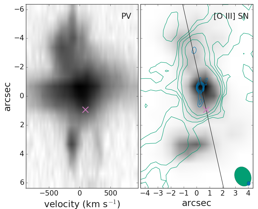 Figure 1
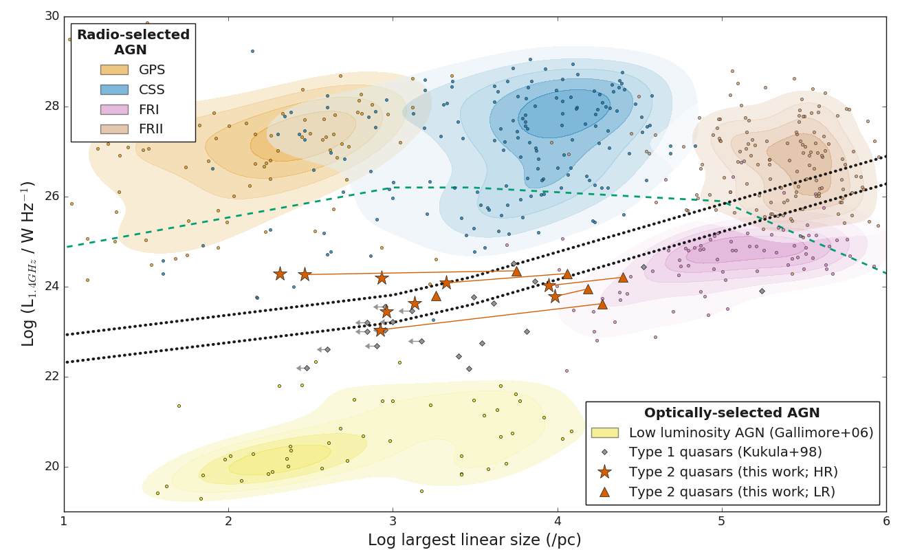 Figure 2
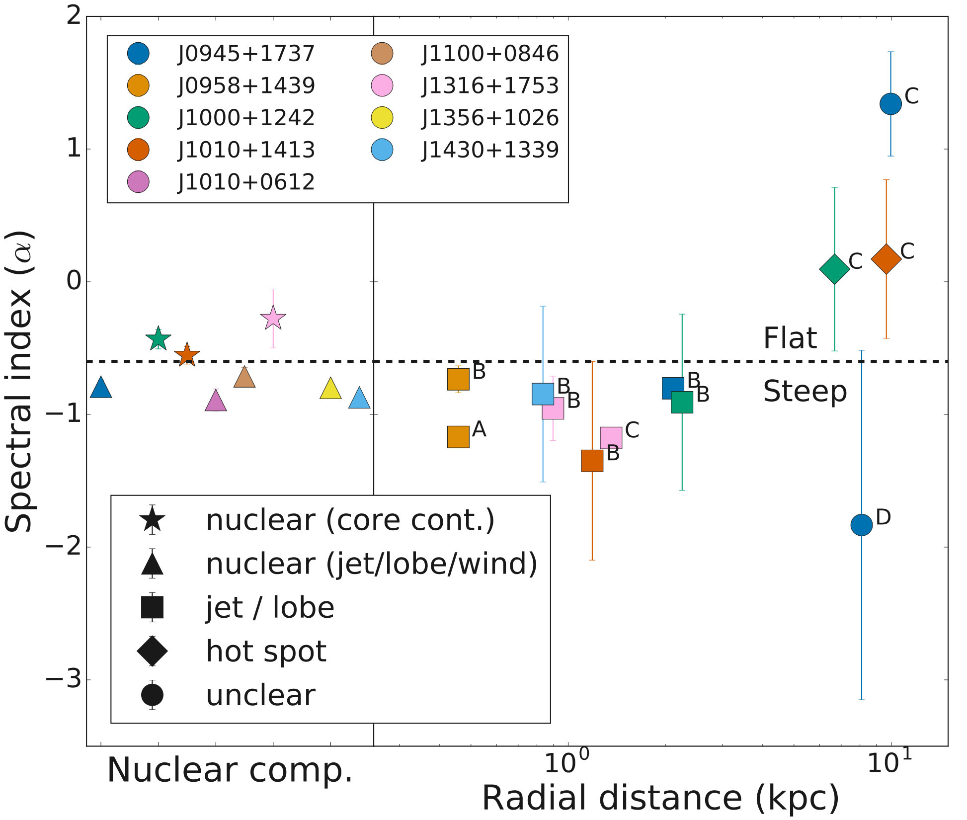 Figure 3
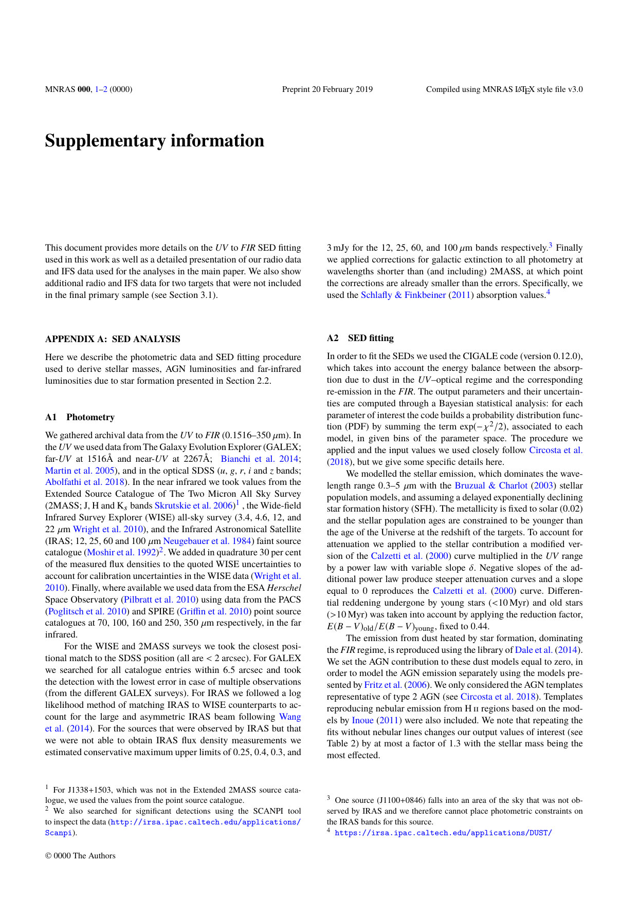 Figure 4
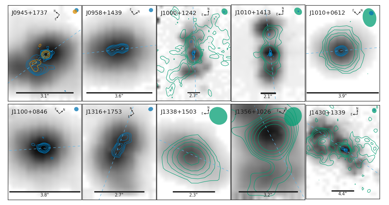 Figure 5
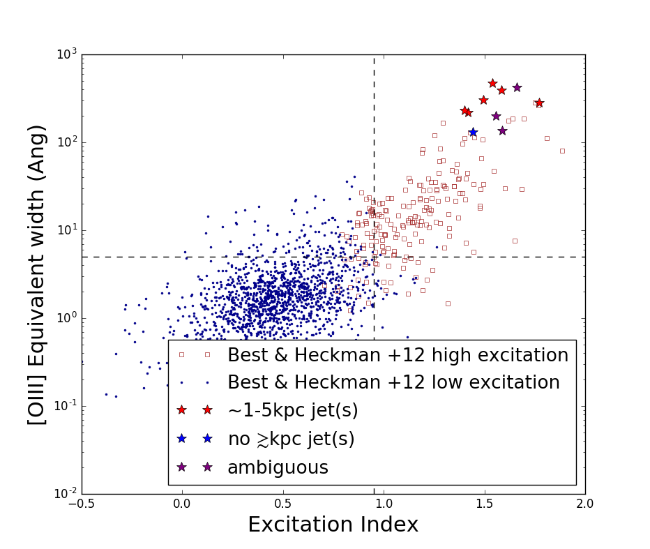 Figure 6
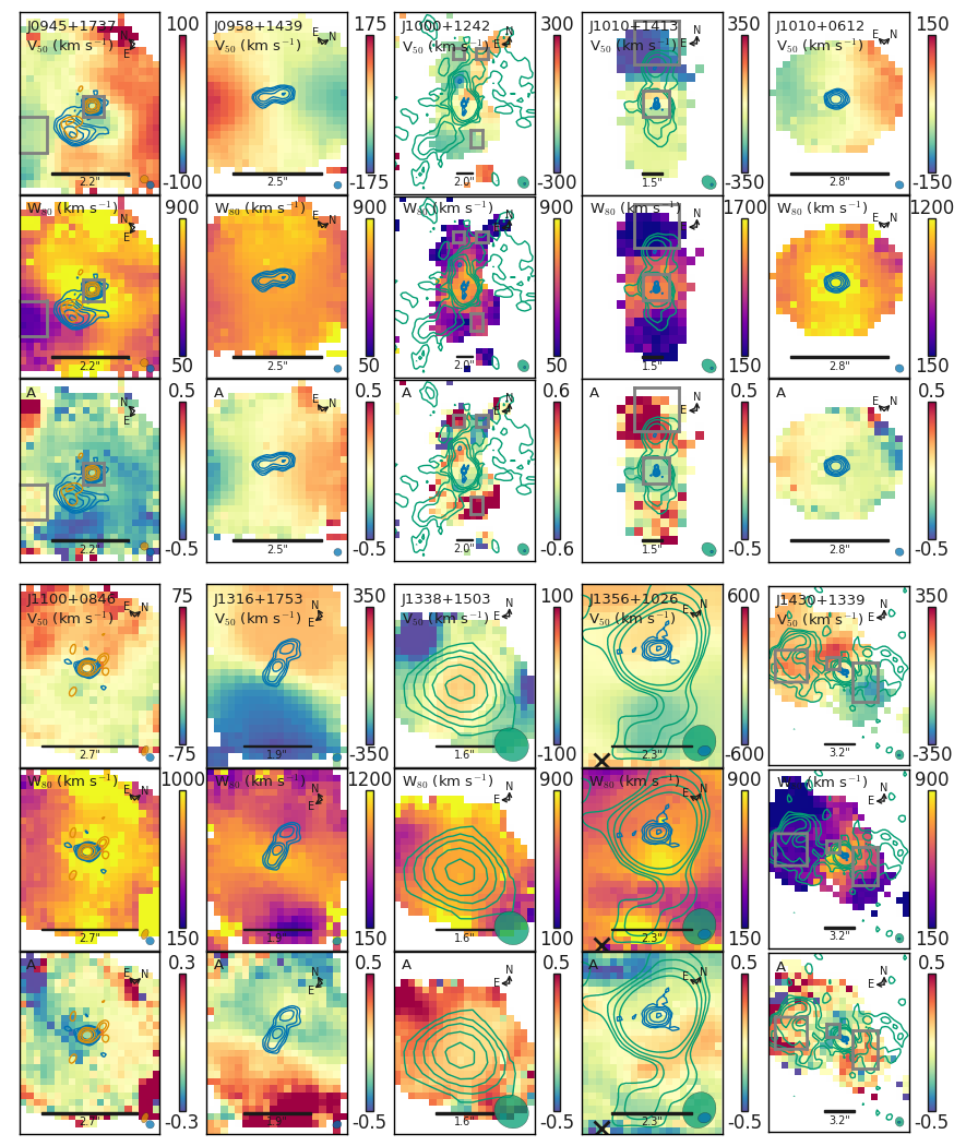 Figure 7
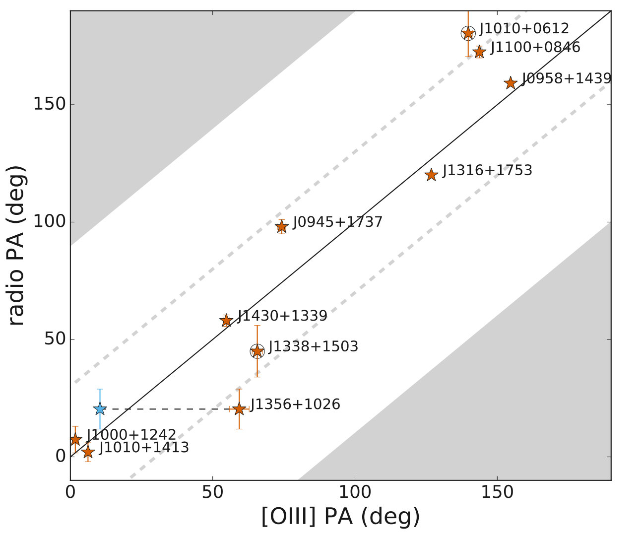 Figure 8
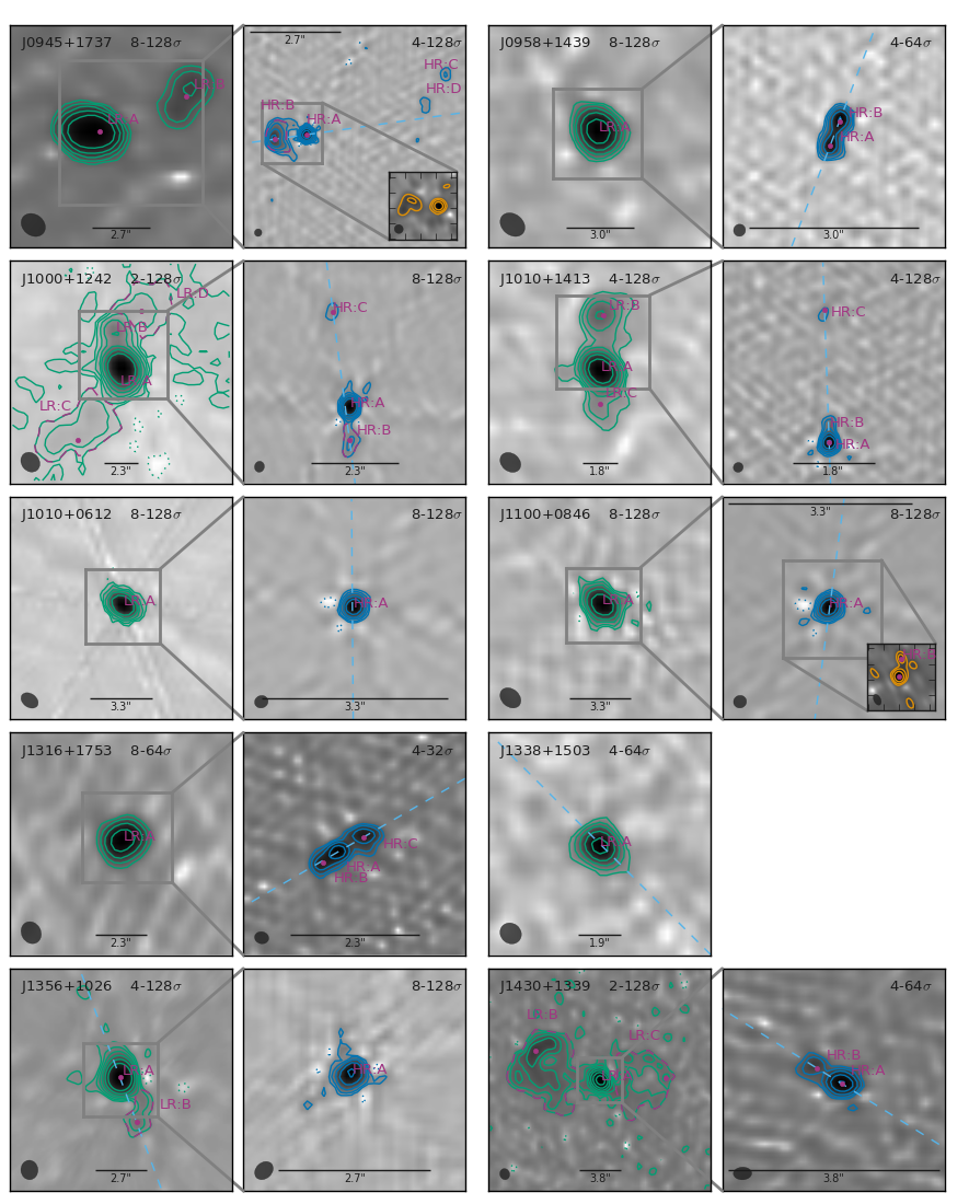 Figure 9
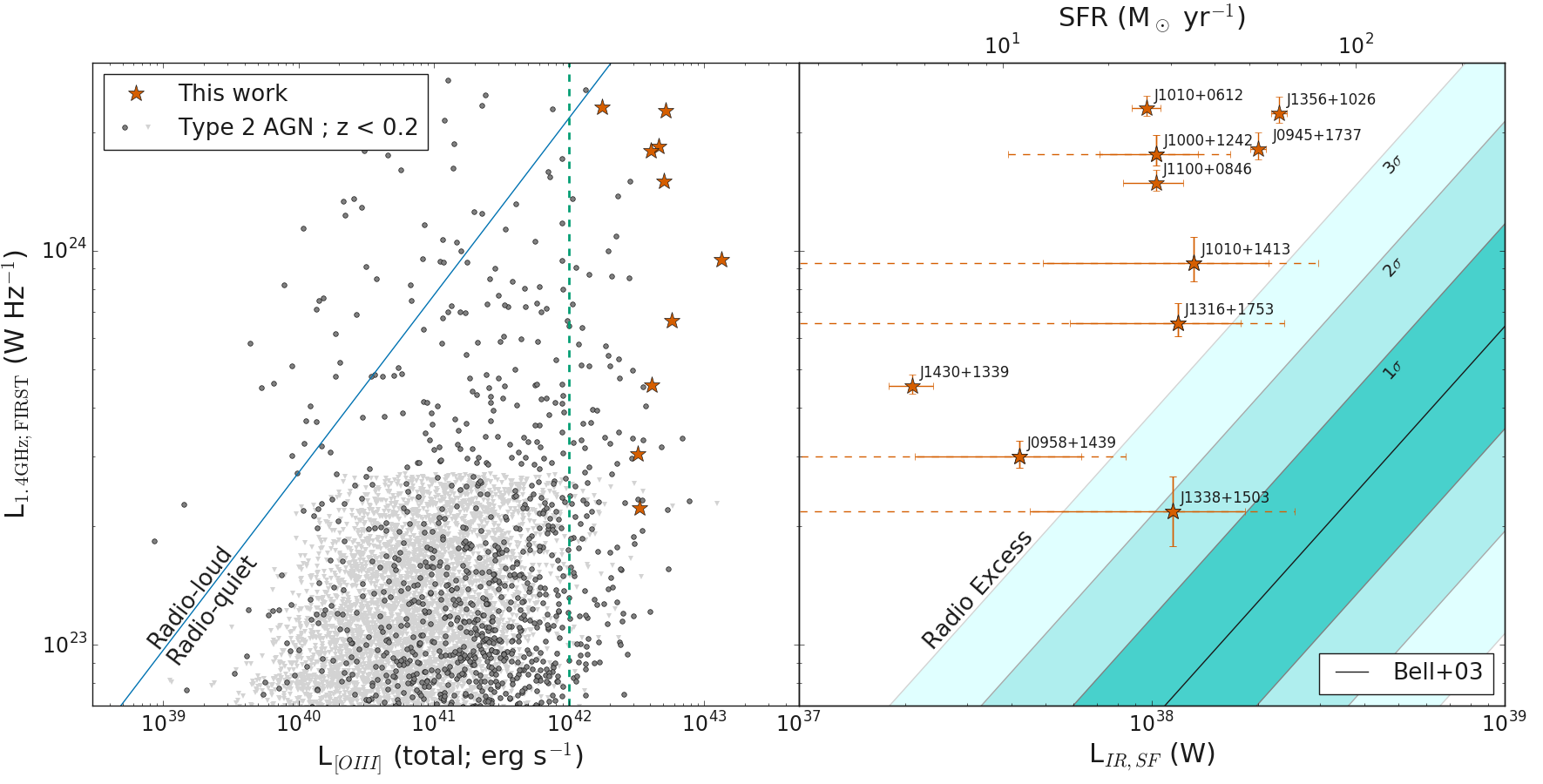 Figure 10
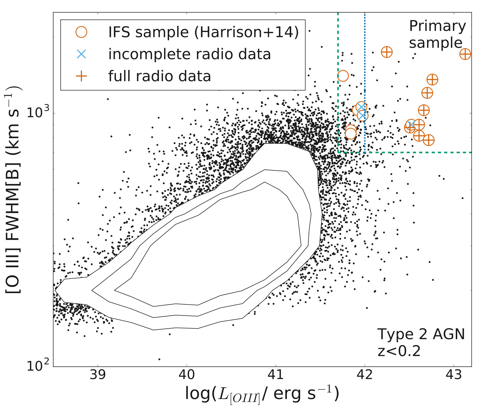 Figure 11
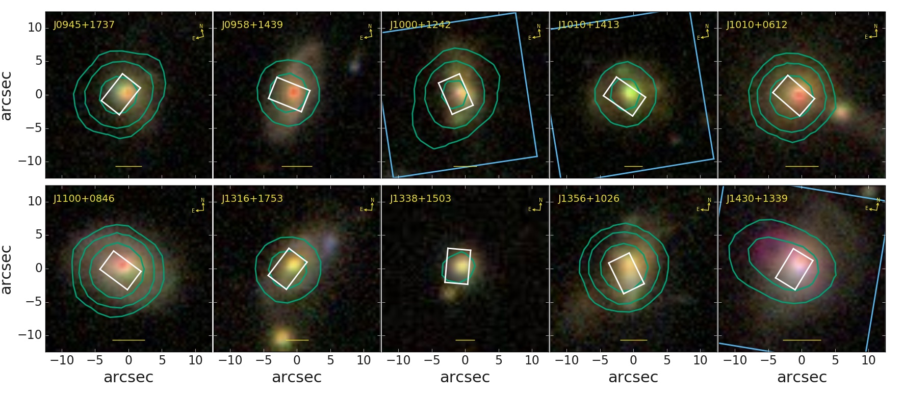 Figure 12
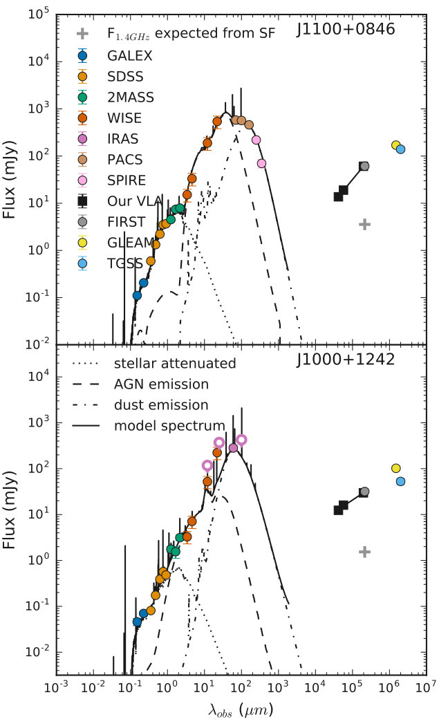 Figure 13
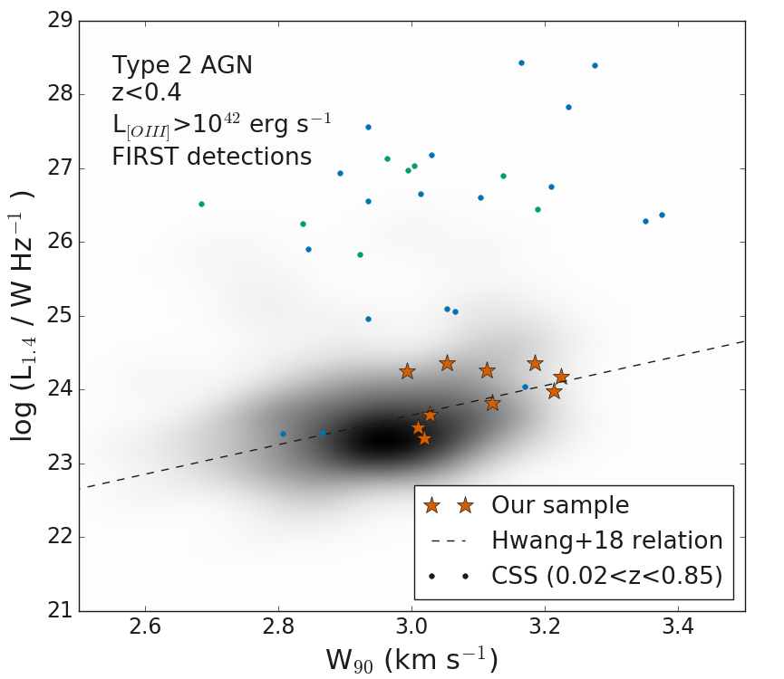 Figure 14
| Name | RA (J2000) | Dec (J2000) | z | FWHM[B] | ||||
|---|---|---|---|---|---|---|---|---|
| (erg s | (km s-1) | (mJy) | (W Hz-1) | |||||
| (1) | (2) | (3) | (4) | (5) | (6) | (7) | (8) | (9) |
| J09451737 | 09:45:21.33 | +17:37:53.2 | 0.1281 | 42.66 | 24.3 | 1.072[3] | ||
| J09581439 | 09:58:16.88 | +14:39:23.7 | 0.1091 | 42.51 | 23.5 | 1.006[9] | ||
| J10001242 | 10:00:13.14 | +12:42:26.2 | 0.1479 | 42.61 | 24.2 | 1.111[4] | ||
| J10101413 | 10:10:22.95 | +14:13:00.9 | 0.1992 | 43.13 | 24.0 | 1.04[1] | ||
| J10100612 | 10:10:43.36 | +06:12:01.4 | 0.0982 | 42.25 | 24.4 | 1.038[3] | ||
| J11000846 | 11:00:12.38 | +08:46:16.3 | 0.1004 | 42.70 | 24.2 | 1.023[1] | ||
| J13161753 | 13:16:42.90 | +17:53:32.5 | 0.1504 | 42.76 | 23.8 | 1.04[1] | ||
| J13381503 | 13:38:06.53 | +15:03:56.1 | 0.1859 | 42.52 | 23.3 | 1.06[5] | ||
| J13561026 | 13:56:46.10 | +10:26:09.0 | 0.1233 | 42.72 | 24.4 | 1.014[2] | ||
| J14301339 | 14:30:29.88 | +13:39:12.0 | 0.0852 | 42.61 | 23.7 | 1.400[9] |
| Name | log[M⋆] | SFR | S | % SF | Radio Excess | |||
|---|---|---|---|---|---|---|---|---|
| (erg s-1) | (M⊙) | (erg s-1) | (M⊙yr-1) | (mJy) | ||||
| (1) | (2) | (3) | (4) | (5) | (6) | (7) | (8) | (9) |
| J0945+1737 | 45.7 | 10.1 | 45.30.02 | 462 | 3.00.2 | 6.90.4 | 1.60.02 | Y |
| J0958+1439† | 45.2 | 10.74 | 44.6 | 105 | 0.90.5 | 94 | 1.7 | P |
| J1000+1242† | 45.3 | 9.9 | 45.0 | 247 | 1.10.4 | 41 | 1.3 | Y |
| J1010+1413† | 46.2 | 11.00.1 | 45.1 | 3020 | 0.80.5 | 95 | 1.8 | P |
| J1010+0612 | 45.3 | 10.5 | 44.990.04 | 222 | 2.60.2 | 2.60.2 | 1.150.04 | Y |
| J1100+0846 | 46.0 | –†† | 45.01 | 245 | 2.60.5 | 4.30.8 | 1.37 | Y |
| J1316+1753† | 44.4 | 11.0 | 45.1 | 3010 | 1.30.6 | 116 | 1.8 | P |
| J1338+1503† | 45.7 | 10.6 | 45.1 | 3020 | 0.80.5 | – | 2.3 | N |
| J1356+1026 | 45.2 | 10.64 | 45.360.02 | 533 | 3.80.2 | 6.40.3 | 1.560.02 | Y |
| J1430+1339 | 45.5 | 10.86 | 44.32 | 4.80.7 | 0.80.1 | 2.90.4 | 1.18 | Y |
| Object Name | Image | Beam HPBW | Beam PA | Noise | Data | Weighting |
|---|---|---|---|---|---|---|
| (arcsec) | (deg) | (Jy/beam) | ||||
| (1) | (2) | (3) | (6) | (7) | ||
| J09451737 | HR | 0.220.21 | C-A | uniform | ||
| J09451737 | LR | 1.170.94 | C-B | briggs 0.5 | ||
| J09581439 | HR | 0.220.21 | C-A | uniform | ||
| J09581439 | LR | 1.220.94 | C-B | briggs 0.5 | ||
| J10001242 | HR | 0.300.26 | C-A | briggs 0.5 | ||
| J10001242 | LR | 1.441.21 | C-A+C-B† | natural & 150k taper | ||
| J10101413 | HR | 0.220.21 | C-A | uniform | ||
| J10101413 | LR | 1.210.95 | C-B | briggs 0.5 | ||
| J10100612 | HR | 0.250.22 | C-A | uniform | ||
| J10100612 | LR | 1.550.93 | C-B | briggs 0.5 | ||
| J11000846 | HR | 0.230.22 | C-A | uniform | ||
| J11000846 | LR | 1.240.94 | C-B | briggs 0.5 | ||
| J13161753 | HR | 0.260.22 | C-A | uniform | ||
| J13161753 | LR | 1.010.86 | C-B | briggs 0.5 | ||
| J13381503 | LR | 1.010.91 | C-B | briggs 0.5 | ||
| J13561026 | HR | 0.370.29 | C-A | briggs 0.5 | ||
| J13561026 | LR | 1.050.92 | C-A+C-B†† | natural | ||
| J14301339 | HR | 0.330.23 | C-A | uniform | ||
| J14301339 | LR | 1.000.88 | C-B | briggs 0.5 |
| Name | S | Structure | Interpretation | ||||
|---|---|---|---|---|---|---|---|
| (mJy) | or LLS | (mJy) | (mJy) | (mJy) | |||
| (1) | (2) | (3) | (4) | (5) | (6) | (7) | (8) |
| J0945+1737 | 44.50.4 | HR:A | nuclear (jet/lobe/wind) | 162 | 6.30.6 | 4.60.5 | -0.790.05 |
| HR:B | jet / lobe | 132 | 4.80.5 | 3.90.4 | -0.80.02 | ||
| HR:C | unclear | 7.5 | 0.240.04 | 0.370.04 | 1.30.4 | ||
| HR:D | unclear | 1.6 | 0.260.04 | 0.150.03 | -21 | ||
| HR:Total | LLS=2.1kpc | 292 | 11.70.9 | 9.00.8 | -0.760.02 | ||
| LR:A | composite | 422 | 131 | 91 | -0.9270.007 | ||
| LR:B | lobe | 4.50.5 | 1.90.2 | 1.40.2 | -0.740.03 | ||
| LR:Total | LLS=11kpc | 471 | 151 | 111 | -0.9060.008 | ||
| J0958+1439 | 10.40.4 | HR:A | jet / lobe | 5.80.7 | 1.30.1 | 0.970.1 | -1.170.07 |
| HR:B | jet / lobe | 3.70.7 | 1.60.2 | 1.20.1 | -0.70.1 | ||
| HR:Total | LLS=0.9kpc | 101 | 2.90.5 | 2.10.4 | -0.9590.001 | ||
| LR:A | composite | 111 | 2.90.3 | 2.10.2 | -1.0570.005 | ||
| J1000+1242 | 31.80.4 | HR:A | nuclear (core cont.) | 202 | 131 | 91 | -0.430.07 |
| HR:B | jet / lobe | 2.1 | 1.00.1 | 0.730.08 | -0.90.7 | ||
| HR:C | hot spot | 1.1 | 0.650.08 | 0.70.1 | 0.10.6 | ||
| HR:Total | LLS=8.9kpc | 201 | 141 | 111 | -0.350.09 | ||
| LR:A | composite | 252 | 141 | 111 | -0.520.05 | ||
| LR:B | lobe | 3.10.3 | 1.20.1 | 1.00.1 | -0.7420.006 | ||
| LR:C | lobe | 1.30.3 | 0.70.1 | 0.60.1 | -0.50.1 | ||
| LR:D‡ | lobe | 0.69 | 0.52 | 0.44 | – | ||
| LR:Total | LLS=25kpc | 301 | 161 | 121 | -0.540.05 | ||
| J1010+1413 | 8.80.5 | HR:A | nuclear (core cont.) | 5.90.7 | 3.20.3 | 2.40.2 | -0.550.07 |
| HR:B | jet / lobe | 2.4 | 0.410.04 | 0.270.03 | -1.30.7 | ||
| HR:C | hot spot | 3.4 | 0.220.03 | 0.230.03 | 0.20.6 | ||
| HR:Total | LLS=9.7kpc | 5.90.8 | 3.80.6 | 2.90.5 | -0.430.1 | ||
| LR:A | composite | 7.50.8 | 3.70.4 | 2.70.3 | -0.630.06 | ||
| LR:B | lobe | 1.10.1 | 0.720.09 | 0.560.06 | -0.430.08 | ||
| LR:C† | lobe | 0.48 | 0.20.04 | 0.270.04 | 0.90.6 | ||
| LR:Total | LLS=15kpc | 8.60.9 | 4.60.6 | 3.60.5 | -0.550.05 | ||
| J1010+0612 | 99.30.3 | HR:A | nuclear (jet/lobe/wind) | 8010 | 303 | 202 | -0.890.08 |
| LR:A | – | 9710 | 293 | 202 | -1.010.05 | ||
| J1100+0846 | 61.30.3 | HR:A | nuclear (jet/lobe/wind) | 425 | 192 | 131 | -0.710.07 |
| HR:B | artefact / variable†† | 203 | 0.1 | 0.13 | – | ||
| HR:Total | LLS=0.8kpc | 622 | 191 | 131 | -0.980.01 | ||
| LR:A | composite†† | 616 | 192 | 141 | -0.950.02 | ||
| J1316+1753 | 11.40.4 | HR:A | nuclear (core cont.) | 1.30.3 | 1.10.1 | 0.830.08 | -0.30.2 |
| HR:B | jet / lobe | 1.80.3 | 0.690.07 | 0.40.04 | -1.00.2 | ||
| HR:C | jet / lobe | 4.20.6 | 0.920.09 | 0.670.07 | -1.180.05 | ||
| HR:Total | LLS=1.4kpc | 7.20.9 | 2.70.4 | 1.90.3 | -0.850.08 | ||
| LR:A | composite | 111 | 3.00.3 | 2.20.2 | -1.0190.001 | ||
| J1338+1503 | 2.40.4 | LR:A | star formation? | – | 0.70.07 | 0.530.05 | -0.90.6 |
| J1356+1026 | 59.60.4 | HR:A | nuclear (jet/lobe/wind) | 495 | 192 | 141 | -0.80.07 |
| LR:A | – | 586 | 202 | 151 | -0.880.03 | ||
| LR:B | unclear | 0.88 | 0.570.07 | 0.40.06 | -1.10.8 | ||
| LR:Total | LLS=5.6kpc | 582 | 211 | 151 | -0.860.03 | ||
| J1430+1339 | 26.40.4 | HR:A | nuclear (jet/lobe/wind) | 6.30.9 | 2.30.2 | 1.60.2 | -0.870.05 |
| HR:B | jet / lobe | 2.1 | 0.690.08 | 0.530.06 | -0.80.7 | ||
| HR:Total | LLS=0.8kpc | 6.30.9 | 2.90.5 | 2.10.4 | -0.690.1 | ||
| LR:A | composite | 121 | 3.40.3 | 2.40.2 | -1.020.01 | ||
| LR:B | lobe | 101 | 3.10.3 | 2.20.2 | -0.970.03 | ||
| LR:C | lobe | 1.80.2 | 0.70.08 | 0.590.07 | -0.720.03 | ||
| LR:Total | LLS=19kpc | 241 | 7.20.7 | 5.20.6 | -0.970.02 |
Peer Reviews
No public reviews on file for this paper yet. If you reviewed it on a platform where reviews are public (OpenReview, ICLR, NeurIPS, ICML), you can paste yours below so the community can read it here.
Videos
No videos yet. Explain this paper in a talk, walkthrough, or lecture? Add one.
Prevalence of radio jets associated with galactic outflows and feedback from quasars
M. E. Jarvis,1,2,3 C. M.Ḣarrison,2 A. P. Thomson,4 C. Circosta,2,3 V. Mainieri,2 D. M. Alexander,5 A. C. Edge,5 G. B. Lansbury,6 S. J. Molyneux2 and J. R. Mullaney7
1Max-Planck Institut für Astrophysik, Karl-Schwarzschild-Str. 1, 85748 Garching, Germany
2European Southern Observatory, Karl-Schwarzschild-Str. 2, 85748 Garching, Germany
3Ludwig Maximilian Universität, Professor-Huber-Platz 2, 80539 Munich, Germany
4Jodrell Bank Centre for Astrophysics, The University of Manchester, Oxford Road, Manchester M13 9PL, UK
5Centre for Extragalactic Astronomy, Department of Physics, Durham University, South Road, Durham DH1 3LE, UK
6Institute of Astronomy, University of Cambridge, Madingley Road, Cambridge, CB3 0HA, UK
7Department of Physics and Astronomy, The University of Sheffield, Hounsfield Road, Sheffield, S3 7RH, UK E-mail: [email protected]
(Accepted XXX. Received YYY; in original form ZZZ)
Abstract
We present 1–7 GHz high-resolution radio imaging (VLA and e-MERLIN) and spatially-resolved ionized gas kinematics for ten type 2 ‘obscured’ quasars (/erg s{}^{-1}]$$\gtrsim$$45) with moderate radio luminosities (/W Hz=23.3–24.4). These targets were selected to have known ionized outflows based on broad [O iii] emission-line components (FWHM800–1800 km s*-1*). Although ‘radio-quiet’ and not ‘radio AGN’ by many traditional criteria, we show that for nine of the targets, star formation likely accounts for 10 per cent of the radio emission. We find that 80–90 per cent of these nine targets exhibit extended radio structures on 1–25 kpc scales. The quasars’ radio morphologies, spectral indices and position on the radio size-luminosity relationship reveals that these sources are consistent with being low power compact radio galaxies. Therefore, we favour radio jets as dominating the radio emission in the majority of these quasars. The radio jets we observe are associated with morphologically and kinematically distinct features in the ionized gas, such as increased turbulence and outflowing bubbles, revealing jet-gas interaction on galactic scales. Importantly, such conclusions could not have been drawn from current low-resolution radio surveys such as FIRST. Our observations support a scenario where compact radio jets, with modest radio luminosities, are a crucial feedback mechanism for massive galaxies during a quasar phase.
keywords:
galaxies: active – galaxy: evolution – galaxies: jets – quasars: general
††pubyear: 2018††pagerange: Prevalence of radio jets associated with galactic outflows and feedback from quasars–Prevalence of radio jets associated with galactic outflows and feedback from quasars
1 Introduction
Growing supermassive black holes at the hearts of massive galaxies, i.e., active galactic nuclei (AGN), are widely believed to be able to impact galaxy evolution by facilitating a global shut-down or regulation of star formation (e.g., see reviews in Alexander & Hickox, 2012; Fabian, 2012; Harrison, 2017). Galaxy formation models require this ‘AGN feedback’ to inject energy or momentum into the surrounding gas, in order to reproduce key observables of galaxy populations and the intergalactic material (e.g., Hopkins et al., 2006; Bower et al., 2006; McCarthy et al., 2010; Gaspari et al., 2011; Dubois et al., 2013; Vogelsberger et al., 2014; Hirschmann et al., 2014; Schaye et al., 2015; Henriques et al., 2015; Taylor & Kobayashi, 2015; Choi et al., 2018).
Historically, ‘AGN feedback’ was considered to come in two flavours: ‘quasar mode’, and ‘maintenance mode’ or ‘radio mode’ (e.g., see Croton, 2009; Bower et al., 2012). The former mode is associated with powerful radiatively-dominated AGN, which are often referred to as quasars (e.g., see Harrison, 2017). The energetic photons are predicted to couple to the nearby gas, resulting in high-velocity winds that propagate through the host galaxy and ultimately in the removal or destruction of the star forming fuel (e.g., Faucher-Giguère & Quataert, 2012; King & Pounds, 2015; Costa et al., 2018). Conversely, maintenance mode is associated with low accretion rate AGN that release most of their energy in the form of radio jets (McNamara & Nulsen, 2012). These jets regulate the cooling of gas in the halos, and hence the level of star formation in their host galaxies. In reality feedback is unlikely to be simply divided into two modes (e.g., Churazov et al., 2005; Ciotti et al., 2010; Cielo et al., 2018) and observations are ultimately required to determine the processes by which AGN impact upon their galaxies.
Observationally, the details of ‘quasar mode’ feedback are not clear. On the one hand, winds driven in the vicinity of the accretion disc are common, if not ubiquitous (e.g., Silk & Rees, 1998; King & Pounds, 2015) and multi-phase AGN-driven outflows have been observed on galaxy-wide scales (i.e., 0.5 kpc) using integral field spectroscopy (IFS) and interferometric observations (e.g., Veilleux et al., 2013; Husemann et al., 2013; Liu et al., 2013; Rupke & Veilleux, 2013; Cicone et al., 2014; Harrison et al., 2014; Fiore et al., 2017; Bae & Woo, 2018; Morganti et al., 2018; Fluetsch et al., 2018). However, determining how these galactic-outflows are driven is challenging; with accretion-disc winds, radio jets and star-formation all potential candidates (e.g., Harrison et al., 2018; Wylezalek & Morganti, 2018).
Whilst radio jets are unambiguously associated with galaxy-wide outflows in rare, extremely radio luminous quasars (i.e., L_{\rm 1.4GHz}$$>1025 W Hz*-1*; Nesvadba et al., 2017); the majority of quasars (90 per cent) have lower radio luminosities. Particularly at moderate luminosities (i.e., 1023\lesssim$$L_{\rm 1.4GHz}$$\lesssim$$10^{25} W Hz*-1*), the dominant origin of radio emission is a matter of ongoing debate (e.g., Condon et al., 2013; Padovani et al., 2015; Zakamska et al., 2004; Zakamska et al., 2016). Furthermore, studies using spatially-unresolved radio emission and spectroscopy are unable to definitively distinguish between winds and radio jets as driving galactic outflows in typical quasars (Mullaney et al., 2013; Villar Martín et al., 2014; Zakamska & Greene, 2014).
As part of an ongoing programme, in this work we use spatially-resolved radio observations and spectroscopy to assess the dominant producer of radio emission and drivers of galactic ionized outflows in quasars. Using a sample of 24,000 AGN we already discovered a strong relationship between the radio luminosity and the prevalence of ionized outflows based on measuring the [O iii] emission-line profiles (Mullaney et al. 2013; also see Zakamska & Greene, 2014; Villar Martín et al., 2014). Here, we combine follow-up high-resolution radio observations and integral field spectrograph observations of ten quasars with moderate radio luminosities.
In Section 2 we describe the sample selection criteria and characterise the sample’s host galaxy and AGN properties, using spectral energy distributions (SEDs). In Section 3 we describe the radio and IFS data sets we used and reduction steps taken and in Section 4 we describe the details of our analyses. In Section 5 we discuss our results in the context of previous work. Finally, in Section 6 we give our conclusions. We adopt =71km s*-1Mpc-1*, =0.27, =0.73 throughout, and define the radio spectral index, , using . We assume a Chabrier (2003) initial mass function (IMF).
2 Target selection and characterisation
2.1 Sample selection
In this work we focus on ten type 2 (‘obscured’) AGN, that have quasar-like luminosities (i.e., L_{\rm[O~{}III]}$$>$$1042 erg s*-1*; Reyes et al., 2008). These were originally selected by Harrison et al. (2014) from our parent sample of 24 264 spectroscopically identified AGN presented in Mullaney et al. (2013). We originally selected 16 sources for follow-up IFS observations that exhibit a luminous broad [O iii] component in the one dimensional spectra, indicative of a powerful ionized outflow (see Fig. 1; Harrison et al., 2014). These IFS data revealed kpc scale ionised outflows. The present text focuses on the subset of ten of these targets with a luminosity of erg s*-1* (referred to as the primary sample; see Fig. 1). In Fig. 2 we show three-colour SDSS images for the ten quasars discussed in this work with the IFS field of view over-plotted.
The positions, redshifts, [O III] properties and radio properties (from the FIRST Survey; Becker et al. 1995) of the ten targets studied in this paper are presented in Table 1. As can be seen in Fig. 3 all of the primary sample discussed here are classified as ‘radio-quiet’ AGN based upon the criteria of Xu et al. (1999). Furthermore, as can be seen from the radio contours from FIRST in Fig. 2, the spatial resolution (5 arcsec) of these data, compared to our IFS observations (i.e., 0.6–0.9 arcsec; Section 3.3), is insufficient to unambiguously relate the kinematic features observed in the IFS data to the radio morphology. This motivated us to observe all of our targets with interferometric radio observations (as described in Section 3) to obtain higher resolution radio images (also see Harrison et al., 2015).
2.2 Star-formation rates and SED fitting
In Fig. 3 we show that all of the quasars in our sample would be classified as ‘radio-quiet’ by the Xu et al. (1999) criterion. However, there is significant debate in the literature as to whether this division marks two populations or one continuous distribution and if these divisions are physically motivated (Cirasuolo et al., 2003; Padovani, 2017; Padovani et al., 2017; Gürkan et al., 2018). A more meaningful measure is to select ‘radio AGN’ by assessing if the observed radio emission is dominated by star formation or by the AGN (e.g. Morić et al., 2010; Best & Heckman, 2012). Although our sources would be classified as star forming by the method of Best & Heckman (2012), the method that we use in this work is to look for an excess of radio emission in relation to the FIR–radio correlation for star-forming galaxies (e.g. Helou et al., 1985; Bell, 2003).
An important consideration in using the FIR–radio correlation to identify so called ‘radio excess’ galaxies is separating the FIR contribution from star formation and the AGN. This is because if both the FIR emission and radio emission are dominated by the AGN, this could produce another correlation, artificially causing AGN to follow the relation set by star-forming galaxies (Morić et al., 2010; Zakamska et al., 2016). We therefore make use spectral energy distribution (SED) fitting from the UV to FIR to isolate the FIR luminosity associated with star formation () in addition to getting stellar masses () and AGN bolometric luminosities (). The details of the archival photometric data we used are provided in the online supplementary information (Appendix A). We note that five of our targets do not have photometric measurements at wavelengths 60m; we flag these targets in Table 2 and assess the reliability of our key parameters for these targets below.
To fit the SEDs we used the Code Investigating GALaxy Emission (CIGALE111https://cigale.lam.fr; Noll et al., 2009; Buat et al., 2015; Ciesla et al., 2015). We followed the basic procedure described in Circosta et al. (2018) but provide specific details of our implementation of the code in the online supplementary information (Appendix A). In short, the code simultaneously fits attenuated stellar emission, dust emission heated by star formation, AGN emission (both primary accretion disc emission and dust heated emission) and nebular emission from the UV to FIR. The code builds up a probability distribution function (PDF) for each parameter of interest, taking into account the variations from the different models. These fits are an improvement on those previously presented in Harrison et al. (2014), most notably, the increased wavelength range used allowed the attenuated stellar emission and dust emission due to star formation to be coupled, increasing the accuracy of , particularly in the cases with limited FIR coverage. Our results show that our targets have that are broadly consistent with luminous infrared galaxies (i.e., 1011 L_{\odot}$$\lesssim$$L_{\rm IR,SF}$$\lesssim$$10^{12} ).
SED fits, especially with limited FUV coverage and an AGN component, can be difficult to determine (see e.g., Bongiorno et al., 2012; Zakamska et al., 2016). Indeed, it is well known that the uncertainties from standard SED-fitting procedures can be artificially small, with the true values being sensitive to, for example, the ‘discretization’ of the template grids used in the fitting procedure. The systematic uncertainties on stellar masses and far infrared luminosities are likely to be around 0.3 dex (Gruppioni et al., 2008; Mancini et al., 2011; Santini et al., 2015). As is important for our interpretation we also tested how reliable our values are for the targets that lack far infrared photometric detections, by re-fitting all of the other SEDs (with good FIR coverage) but removing the longer wavelength data. Through this exercise we find that even with no data at 22m, the new values vary by no more than from the values derived using all the available FIR data222 is the formal error recorded in Table 2.. This is likely due to the additional constraints on the star formation that come from the optical part of the SEDs in our fitting procedure. These boosted (2) errors also make the values consistent with the values presented for the same sources in Harrison et al. (2014). We flag these affected sources in Table 2 and show the error bars in Fig. 3. We note that these additional systematic uncertainties do not affect the conclusions drawn in this paper.
To estimate the star formation rates of our targets we used the SED-derived and the relationship from Kennicutt & Evans (2012), correcting to a Chabrier IMF by dividing by 1.7 (Chabrier, 2003). In Table 2 the quoted uncertainties are only from the SED-derived uncertainties. We note that there is an additional systematic uncertainty on the star formation rates due to the conversion factor from the far-infrared luminosity (i.e., 0.3 dex; Kennicutt & Evans, 2012).
Our targets are type 2 AGN, and consequently, we do not detect the primary AGN disc emission in the UV–optical part of the SED. Therefore, to estimate the bolometric AGN luminosity () we converted the 6m luminosity from the AGN emission component using a bolometric correction of 8 following Richards et al. (2006). The uncertainties on these values are dominated by a 1 dex systematic uncertainty on the bolometric corrections. This confirms that our targets are consistent with having quasar luminosities (i.e., L_{\rm AGN}$$\gtrsim$$10^{45} erg s*-1*)333We note that the bolometric luminosity calculated in this way is below the quasar limit for J13161753, however it is consistent with being equal to or above 1045 erg s*-1* within the 1 dex error mentioned above. Additionally, it is clearly a quasar using the [O iii] luminosity (Reyes et al., 2008)., which we also find by using and the bolometric correction from Heckman et al. (2004) (see Table 2).
Two example SEDs are shown in Fig. 4 and the remainder are provided in online supplementary material. Although the SEDs are only fit using the UV–FIR photometry we also show the radio fluxes from three radio surveys, when available: FIRST (1.4 GHz); TIFR GMRT Sky Survey Alternative Data release (TGSS; 150MHz; Intema et al., 2017); and the GaLactic and Extragalactic All-sky MWA Survey (GLEAM; 200MHz; Hurley-Walker et al., 2017), as well as the total flux from our measurements at 1.5, 5.2 and 7.2 GHz (see Section 4.1.1 and Table 4). These additional radio data allow for visual comparison to the level of emission expected from star formation alone (Bell, 2003) and the identification of spectral turnovers in the radio SEDs (Section 5.2.3).
In Fig. 3 we show as a function of radio luminosity (see Table 1) for our targets and compare these values to the FIR–radio correlation of star-forming galaxies from Bell (2003). It can be seen that nine of our ten targets lie well above the FIR–radio correlation444If we instead used the FIR–radio correlation from Delhaize et al. (2017) the nine targets lie even further above the relationship of star-forming galaxies. (the exception is J13381503). We note that for three of the targets, which all have poor FIR photometry, the uncertainties could cause them to be consistent with star-forming galaxies, within the 3 scatter on that relation, and we highlight these targets in Table 2. However, based on our spatially-resolved radio images presented in Section 3.1.2, we are confident that these sources have significant radio emission that is not associated with star formation. The distance of points from this relation can be quantified using the parameter, defined as
[TABLE]
where is the rest-frame far-infrared (8–1000 m) luminosity, and sources with are considered radio excess (see Table 2; e.g. Bell, 2003; Del Moro et al., 2013; Delhaize et al., 2017).
In Table 2 we also show the radio flux that we expect from star formation following Bell (2003) and we find that for our nine ‘radio excess’ targets, the star formation is expected to contribute 3–11 per cent of the total observed radio emission (also see Fig. 4). We discuss this in more detail in Section 5.2.1.
3 Observations and data reduction
3.1 VLA observations, and imaging
3.1.1 Observations and data reduction
We observed with VLA under two proposals: programme 13B-127, with observations carried out 2013 December 1– 2014 May 13 and programme 16A-182 with observations carried out 2016 May 30 – 2017 January 20. For 13B-127 we observed nine targets, from our primary sample of ten, in four configuration–frequency combinations: (1) A-array in L-band (1–2 GHz; 1.3 arcsec resolution); (2) A-array in C-band (4–8 GHz; 0.3 arcsec resolution); (3) B-array in L-band (1–2 GHz; 4.3 arcsec resolution) and (4) B-array in C-band (4–8 GHz; 1.0 arcsec resolution). The final target in our primary sample (J13381503)555along with two other targets from the Harrison et al. (2014) sample not included in the primary sample (J13551300 and J15040151; see supplementary information), was observed by VLA during our 16A-182 project. Due to incomplete observations, this was only observed in one configuration–frequency combination: B-array configuration in the C-band (i.e., 4–8 GHz; 1.0 arcsec resolution).
The 13B-127 observations comprise 2 hours (5 minutes on each target) of L-band observations in the A-configuration, and 2.5 hours (7–10 minutes on each target) of L-band observations in the B-configuration. For the C-band, 2.5 hours (7 minutes on each target) and 2 hours (5 minutes on each target) of observations were taken in A- and B-configurations, respectively. During our 16A-182 observations C-band data in B-configuration were taken of three targets. These were taken with 2 or 3 repeats of 1 hour observing blocks (with 35, 32 and 26 minutes on target for each J13381503; J13551300 and J15040151, respectively).
We perform amplitude and bandpass calibration at L- and C-band at the start of each observing block using a 10 minute scan on the standard calibration source J1331+3030 (3C 286), and determine complex gain solutions via 3 minute scans (including slew-time) of nearby calibration sources every – minutes (typically within 10∘ of our targets). We choose calibration sources from the list of VLA calibrators website666https://science.nrao.edu/facilities/vla/observing/callist with codes which deem them suitable for each combination of array configuration/observing frequency. The 13B-127 observations were reduced using the Common Astronomy Software Applications (casa777https://casa.nrao.edu/) package (version 4.1.0), along with version 1.2.0 of the VLA scripted pipeline. We reduced the later 16A-182 observations using casa version 4.5.2, and version 1.3.5 of the VLA scripted pipeline.
3.1.2 Imaging
When imaging the VLA data we had two goals: (1) identify any morphological features that are present in the radio emission and (2) measure the fluxes / spectral indices of these features. These goals required different approaches to the imaging of the data and we describe them both here. In order to take into account the broad and varying bandwidths of our observations, all of the VLA images we present were made using the Multi-Frequency Synthesis (MFS) mode of the clean function in casa version 4.7.1. We chose the weighting of the baselines to obtain the desired compromise between sensitivity and beam size to achieve our science goals (see Briggs 1995). In some cases we additionally applied Gaussian tapering to achieve the desired resolution. Because of the relatively short observing times of our targets and resultant limited coverage our cleaned images sometimes still suffer from relatively strong beam residuals. However, in order to test the validity of these features we ensured that they were identified at multiple frequencies and using different combinations of weighting and tapering (see Section 4.1.1).
For our first goal, we aimed to identify both diffuse and compact morphological features in the radio emission. To do this we made two C-band (6 GHz) ‘showcase images’ for each galaxy in the primary sample: one with a 1 arcsec beam (i.e., 2 kpc at =; referred to as ‘low-resolution’ or LR) and one with a 0.25 arcsec beam (i.e., 0.5 kpc at =; referred to as ‘high-resolution’ or HR)888For J13381503 only a low-resolution image was created due to there being no available A-configuration VLA data.. Fig. 5 shows the low and high-resolution images for each source. For these showcase images, the imaging parameters (weighting, tapering and concatenating data sets) were tweaked to best reveal the morphological features found in each galaxy (details in Table 3). The (noise) values are calculated using 8 clipping repeated ten times across a region of the images that is 50 times the size of the beam major axis.
For our second goal we measured the flux densities and spectral indices (over 1-7GHz) for each morphological feature identified. To do this we required multi-frequency images with the same spatial resolution. We produced images at 1.5, 5.2 and 7.2 GHz, where the 5.2 and 7.2 GHz images were made by evenly splitting the 16 VLA C-band spectral windows. We created two sets of these resolution-matched multi-frequency images using weighting and tapering to match the beams as closely as possible, one set at high-resolution (0.25 arcsec; using e-MERLIN for the 1.5 GHz data; see Section 3.2) and one set at low-resolution (1 arcsec; using the VLA L-band A-configuration data for the 1.5 GHz images). Full details of the data used, applied weighting schemes/tapering, the resultant properties of the images (i.e., beam sizes, noise levels; see Table B1) and all 56 of these images, are presented in the online supplementary material.
For the two sources observed with our VLA 16A-182 programme but not included in the primary sample (J13551300 and J15040151), the details of the imaging, the images themselves and a brief discussion of the features seen are presented in the online supplementary material (Appendix C).
3.2 e-MERLIN observations and imaging
We obtained 1.5 GHz (L-band) e-MERLIN observations with 40–172 minutes on-source per target in Cycle 1 (ID: CY 1022; observed on 2013 December 19) and 1.5–3 hours on-source per target in Cycle 2 (ID: CY 2217; observed between 2015 January 21–23). Each observing block entailed 30 minute scans of + and + for flux density and bandpass calibration, respectively. Target scans were 8 minutes, interspersed with 3 minute scans of bright, nearby phase reference sources. We processed the data in aips version 31dec15, with most steps being carried out using the e-MERLIN pipeline (Argo, 2015), but with extensive additional manual flagging of bad data using the aips tasks spflg and ibled.
We created pixel maps from our calibrated data using imagr with a pixel size of 0.05 arcsec (i.e. a 3 arcminute postage stamp around each source), and iteratively deconvolved the point spread function (PSF) within manually-defined clean boxes around sources of bright emission. Our typical synthesised beam is 0.2–0.3 arcsec and in all cases the beams have axial ratios of .
Unfortunately, a combination of strong, persistent radio frequency interference (RFI) and hardware failures resulted in the loss of 50 per cent of our Cycle 1 data, covering both target and calibrator fields. The resulting loss of point-source sensitivity and coverage severely limited the quality of the final images, leaving us unable to achieve our science goals of establishing the radio morphologies at 1.5 GHz. Consequently we do not use these data in our analyses. Fortunately, only one of our primary targets (J13381503) was part of this Cycle 1 programme. Improvements in both the hardware performance and observing strategies for Cycle 2 lowered our loss-rate to 20 per cent (with significantly improved coverage), yielding improved imaging (Jy beam*-1*) and allowing us to study the 1.5 GHz morphologies on sub-kpc scales of the nine of our primary targets, that were all observed in this cycle.
3.3 IFS observations and data reduction
All of our quasars have published IFS data obtained using Gemini-GMOS (Harrison et al., 2014). These observations covered the O [iii]4959, 5007 and H emission-lines using 25 20 lenslets sampling a 5 3.5 arcsec field of view. The spectral resolution of 3700 gives a line FWHM of 80 km s*-1*. The observations were performed with a typical V band seeing of 0.7 arcsec. More details about these observations are given in Harrison et al. (2014).
As part of an uncompleted ESO programme, three of our targets (J14301339, J10101413 and J10001242) also have IFS observations with VIMOS on the ESO/VLT telescope observed from 2014 January 23–24 and 2014 March 9–10 (Program ID: 092.B-0062). The VIMOS observations, which benefit from a 2020 arcsec field of view, were motivated by the kinematic and morphological structures that appeared to extend beyond the GMOS field of view (i.e., on 5 arcsec scales; Harrison et al., 2014, see Fig. 2). The data for J14301339 are already published in Harrison et al. (2015) and we combine these data with the rest of the sample here.
We used VIMOS in IFS mode, using the HR-Orange grism, which provides a wavelength range of 5250–7400Å at a spectral resolution of 2650, giving a line FWHM of 110 km s*-1* at 5007Å, which we confirmed within 10 km s*-1* by measurements of sky-lines. During the observations the targets were dithered around the four quadrants of the VIMOS field of view. The on-source exposure times were 6480 seconds for J14301339 and J10101413; and 2160 seconds for J10001242. The V-band seeing ranged between 0.8–0.9 arcsec. Standard stars were taken under similar conditions to the science observations. The standard esorex pipeline was used to reduce the data, which includes bias subtraction, flat-fielding, wavelength calibration and flux calibration. Data cubes were constructed from the individually sky-subtracted, reduced science frames. The final data cubes were created by median combining the individual exposure cubes using a three-sigma clipping threshold.
4 Analyses
Here we describe the techniques used to identify and characterise morphological and kinematic features observed in our radio and optical IFS data. In Section 4.1 we identify the radio features seen at different resolution and measure the location, flux and spectral index for each feature. In Section 4.2, we describe the non-parametric characterisation of the [O iii] emission-line profiles and explain how we produced emission-line kinematic maps.
4.1 Radio analyses
4.1.1 Radio features, flux densities and spectral indices
As can be seen in Fig. 5 our sources are typically composed of multiple spatially-distinct radio features. In order to constrain the source of the radio emission in each of these morphological features (discussed in Section 5.2), we calculated flux densities and spectral indices for each. We note that we tested our overall approach to flux calibration and to obtaining flux densities by verifying that the total fluxes of the sources from our imaged VLA L-band B-array data (average spatial resolution of 4.3 arcsec) are consistent with the FIRST values (5 arcsec beam) within errors. We note that the variations in flux densities by converting between the difference in the central frequency of our observations and FIRST (i.e., 1.5 GHz to 1.4 GHz) is smaller than the errors on our fluxes.
We name each morphologically distinct feature (detected at 3) in the high-resolution images as HR:A, HR:B etc., and similarly for the low-resolution images with LR:A, LR:B etc. For the low significance features (e.g. HR:C in J10001242) we verified that they are real by ensuring that they were significantly detected in images produced using multiple weighting schemes and/or in independent observations. In general the e-MERLIN images (see Section 3.2) did not reveal any new information on the morphological features. The exceptions are: for J09451737, where the HR:B feature shows a bent ‘jet like’ appearance in the e-MERLIN image; and for J11000846, which shows a 7 feature (HR:B; see Table 4) in the e-MERLIN image that is not identified in the 6 GHz VLA images. We show the e-MERLIN images for these two sources in Fig. 5. The e-MERLIN images for all sources are presented in the supplementary online material. We discuss the origin of the identified radio features in Section 5.2.
Due to the range of morphologies seen in our data (see Fig. 5), we were required to use two approaches to obtain the flux densities of each feature. The first approach was to model the emission as a series of two-dimensional Gaussian components. All of the parameters of the fits were left free999For the LR-C component of J10101413 we were required to fix the peak position of the Gaussians to within 0.5 pixels to obtain a reasonable fit. We flag this feature as having unreliable flux density measurements.. We note that the feature LR:A in both J09451737 and J10001242 needed two component Gaussians to provide an adequate fit, which is easily explained by the multiple HR components that they are composed of (see Fig. 5).
The second approach was to sum the emission in regions motivated by the lowest-level contours of the appropriate resolution image in Fig. 5. We verified that the flux density measurements are consistent within the errors (described below) if we vary the defined region sizes up or down by 25 per cent. These regions were primarily used for diffuse/irregular structures that are not well described by a Gaussian and are referred to as ‘region components’. Where it was possible to apply both approaches, we further verified that they gave consistent results, but favoured the Gaussian fitting method. In the cases where a compact nuclear component was seen in addition to a more diffuse structure, the flux in the diffuse regions was calculated after subtracting off the Gaussian fits to the compact component(s) in order to minimize contamination. Figures showing the data, our best-fit models and the corresponding residuals for all multi-frequency images can be found in the online supplementary material.
To calculate the random noise on our flux density measurements for each feature, we took the standard deviation of 100 repeats of extracting flux densities from inside appropriately sized regions randomly positioned within the central 10 arcsec (for high-resolution images) or 20 arcsec (for the low-resolution images) avoiding source emission. For the ‘region components’ the regions used in this procedure were the same size and shape as those used to extract the flux densities. For the Gaussian components we used an ellipse with axis sizes equal to twice the semi-minor and semi-major axes of the fits. To establish if a feature was detected in each of the 1.5, 5.2 and 7.2 GHz images, we imposed a 5 detection limit. For each of the detected components, we added an additional 10 per cent systematic error, in quadrature, to the uncertainties to account for the random variations we found when extracting flux densities when changing the weighting scheme used to image the data. The final flux densities (or 5 upper limits) and their 1 uncertainties at 1.5, 5.2 and 7.2 GHz are presented in Table 4.
The spectral index (, which we define as ) is used to help interpret the source of the radio emission for each feature in Section 5.2. We measured this by fitting a line through all of the detected frequencies (1.5, 5.2 and 7.2 GHz) for each radio structure. The errors given for in Table 4 are the 1 errors on the fit, except for where the component was only detected in two bands, then the error is the propagated error from the two measured fluxes. Some of our data were observed at different epochs (e.g., when combining our e-MERLIN and VLA C-band B-configuration data) which risks unknown variability of the fluxes affecting the spectral index values. However, we find that our values are consistent to those calculated using only our single-epoch VLA C-band data (within the errors on the VLA C-band values). The 1-7 GHz radio SEDs for each radio component are presented in the supplementary material. The spectral indices for the high-resolution components are plotted in Fig. 6 along with their distance from the central brightest component (HR:A; see Section 4.1.2).
4.1.2 Radio sizes and position angles of the major axes
Here we provide two quantitative measures of the large scale radio morphology for each source: (1) the largest linear size (LLS) and (2) the position angle of the major axis. For the size measurements, our method is motivated by comparing to published radio sizes for other samples (see Section 5.2.3). Therefore, for both the high and low-resolution showcase images (Fig. 5) the largest linear size is calculated as the distance between the peak emission of the two farthest morphological features (see e.g. Kunert-Bajraszewska et al., 2010). For the features well described by Gaussian components the peak of the Gaussian fits are used and for region components the brightest pixel within the region is used to motivate the peak position. These peak positions are shown as magenta points in Fig. 5. For the components with only one observed morphological feature in our highest resolution radio images (J10100612, J13381503 and J13561026) we used casa’s imfit function to calculate the deconvolved size. The sizes used for these components are the major axis size from these fits which are 1157.8 marcsec (0.2 kpc), 59541 marcsec (2 kpc) and 13334 marcsec (0.3 kpc) respectively. We plot all these sizes in Fig. 7.
To obtain the position angle of the major axis of the radio emission, we defined an axis by a line connecting the two peaks used to calculate the largest linear sizes. To check for consistency with the method used to calculate the position angle of the ionized gas emission (see Section 4.2), and to estimate the reliability of these position angles, we fit two dimensional Gaussians to the showcase image (Fig. 5) of each target after first applying a Gaussian filter with arcsec101010For J11000846 we used the e-MERLIN image for this and only burred by a arcsec Gaussian filter so as to not completely remove the effect of HR:B.. We then used the difference between the fit PA and that from connecting the two farthest peaks as an error on the position angle. These errors are between 0.2 and 9∘ (in all cases this was larger than the formal error on the fit). In most cases, the high-resolution radio images were used to identify the positional angle. The two exceptions are J13381503 (where we have no high-resolution image) and J13561026 where an extended feature is only visible in the low-resolution image. In the two cases where no extended radio features were identified in any of our radio images (J10100612 and J13381503), the two-dimensional fit in casa was used to identify the deconvolved PA and its error. These radio major axes are indicated by the blue dashed lines in Fig. 5.
4.2 Ionized gas maps and analyses
Here we describe the steps taken to analyse the ionized gas morphologies and kinematics using our optical IFS data from GMOS and VIMOS (see Section 3.3), and how we align these data to our radio maps. We trace the ionized gas kinematics using the [O iii] emission-line profile and follow the procedures described in detail in Harrison et al. (2014); Harrison et al. (2015), with brief details given here.
To map the dominant gas kinematics across the galaxies and compare to the radio morphologies, following Harrison et al. (2014); Harrison et al. (2015), we use the following non-parametric definitions to characterise the overall [O iii] emission-line profiles:
The peak signal-to-noise ratio (S/N), which is the S/N of the emission-line profile at the peak flux density. This allows us to identify the spatial distribution of the emission-line gas, including low surface-brightness features. 2. 2.
The ‘median velocity’ (), which is the velocity at 50 per cent of the cumulative flux. This allows the ‘bulk’ ionized gas velocities to be traced. 3. 3.
The line width, , which is the velocity width that contains 80 per cent of the overall emission-line flux. This characterises the overall width of the emission-line, irrespective of the underlying profile shape. For comparison to other work (Section 5.4) we also calculate , which contains 90 per cent of the overall emission-line flux. 4. 4.
The asymmetry value (; see Liu et al., 2013), which is defined as:
[TABLE]
where and , are the velocities at 10 per cent, and 90 per cent of the cumulative flux, respectively. A very negative (positive) value of means that the emission-line profile has a strong blue (red) wing.
To minimize the effect of noise on the broad wings of the emission-lines even in regions of low S/N, we fit the [O iii]4959,5007 emission-line profile with multiple Gaussian components, correcting for the instrumental dispersion, following the methods described in Harrison et al. (2014); Harrison et al. (2015). We produce maps of each of the parameters described above by fitting the emission-line profiles in 0.6 arcsec spatial regions (i.e., comparable to the seeing of the observations). The (S/N) maps are shown in Fig. 8 and the other maps are presented in Section 5.3.
The systemic redshifts quoted in Table 1 are derived using the values of the [O iii] emission-line profiles extracted from a 33 arcsec aperture centred on the quasar’s SDSS position in the GMOS data cubes. This corresponds roughly to the velocity of the narrow component, which is often attributed to galaxy kinematics (e.g. Greene & Ho, 2005; Rupke & Veilleux, 2013) or in the case of multiple peaks, lies roughly at the central velocity which, assuming the peaks are dominated by either rotation or symmetric outflows (e.g. Holt et al., 2008), should give a good estimate of the systemic velocity. We note that the values used here vary from the quoted SDSS redshifts by a maximum of 100 km s*-1*.
To compare the morphology of the ionized gas quantitatively to our radio images, we measure a position angle from our S/N maps. We define the major axis of the [O iii] emission by fitting a single Gaussian to the S/N map for each galaxy. This method is slightly biased to passing through the brightest features in the [O iii]; however, based on visual inspection provides a sufficient measurement of the position angle for our broad comparison to the distribution of radio emission presented in Section 5.3. The main exception is J13561026 for which the position angle we measure for the ionized gas is determined primarily by a bright region to the north east of the core with no radio counterpart observed. However, if we define the position angle using the location of the base of the bubble identified by Greene et al. (2012) (see Section 5.3), the radio and [O iii] emission are well aligned, with a PA separation of 10 degrees. These positional angles are shown on the [O iii] S/N maps in Fig. 8 and are plotted against the radio PAs in Fig. 9.
We aligned the IFS data to the SDSS astrometry by creating pseudo-broad band images from the IFS cubes using the common wavelength coverage with SDSS r band111111for J13381503 the g band filter was used because the r was too effected by bad pixels near the edge of the IFS wavelength range.. We then anchored the astrometric information of the IFS peak pixel location to the associated position from the SDSS image peak, after blurring each with a 0.2 arcsec Gaussian filter to minimize the impact of bad pixels. We used the brightest morphological components in our high-resolution VLA images (HR:A) to confirm that the SDSS and VLA astrometry were consistent121212J09581439 was excluded from this since it seems likely, due to their similar brightness and steep spectral indices, that both of the radio components in this source are lobes around a central, core below our detection threshold.. We found the SDSS positions were scattered around the peak VLA emission with a median offset of 0.13 arcsec, corresponding to 0.24 kpc at a representative redshift of =0.1. This is sufficient for the comparison we make between the radio morphologies and our 0.6–0.7 arcsec resolution ionized gas kinematics in this work (Section 5.3).
5 Results and discussion
In the previous section we presented our 1–7 GHz radio imaging and optical integral field spectroscopy for a sample of ten z$$<$$0.2 ‘radio-quiet’ quasars, that were known to host kpc-scale ionized outflows based on our previous work (Fig. 8; Harrison et al., 2014; Harrison et al., 2015). The aim of this section is to establish the origin of the radio emission (Section 5.1 and Section 5.2), to explore the relationship between the radio and the ionized gas (Section 5.3) and to discuss the implication of our results for understanding the radio emission and feedback in the context of the overall AGN population (Section 5.4).
5.1 Properties of the observed radio emission
We observe radio structures with a range of morphologies from compact features with spatial extents of 1 kpc (e.g., see the high-resolution image of J09581439 in Fig. 5) to diffuse lobes extending over 25 kpc (e.g., see the low-resolution radio image of J10001242 in Fig. 5). In particular five of our targets show distinctly jet like radio morphologies (J09451737, J09581439, J10001242, J10101413 and J13161753) with three more showing more irregular radio features (J1100+0846, J1356+1026 and J1430+1339; see Section 5.2.4 and Harrison et al., 2015). Specifically, this means that of the nine quasars in the sample consistent with being radio excess in Section 2.2 (i.e. all except J13381503; see Fig. 3 and Table 2) 90 per cent show spatially resolved radio structures with linear sizes on 1–25 kpc scales (see Fig. 5 and Fig. 7).
To estimate the significance of the features that we have identified in our high-resolution VLA and e-MERLIN data in terms of their contribution to the total radio luminosity at 1.5 GHz, we compare the radio emission from these morphologically-distinct features to the total radio emission (extracted from FIRST but consistent with our observations, see Section 4.1.1; Table 1). For the radio excess sources, we find that the total combined fluxes of the high-resolution components, including the central nuclear components, (i.e., HR:Total in Table 4) contain 60–90 per cent of the total radio flux. The exception is J14301339 for which the high-resolution components only make up 22 per cent of the total flux with 50 per cent of the FIRST flux located in the diffuse low-resolution lobes/bubbles. Below, we discuss how the radio emission that is resolved out on these 0.25 arcsec scales may be attributed to star formation.
Importantly, as can be seen by eye in Fig. 2 and quantitatively using the parameter (see Table 1), only J14301339 is definitively extended and two other sources (J09451737 and J10001242) are tentatively extended based upon their 5 arcsec resolution FIRST data. This is supported by the ‘FIRST Classifier’ (Alhassan et al., 2018), which automatically identifies FIRST sources as compact or not, and determines that all of our sources are compact except for J14301339. This cautions against only relying on low-resolution radio data to identify low power/compact radio structures not associated with star formation in such systems (e.g., see Kimball et al., 2011; Le et al., 2017).
5.2 Origin of the radio emission
5.2.1 Star formation
All of our targets are classified as being ‘radio-quiet’ based on standard criteria (e.g., Xu et al., 1999, see Fig. 3). Furthermore, based on many standard criteria, our sources would not be classified as ‘radio AGN’ (e.g., Best & Heckman, 2012, Section 2.2). The radio emission in such sources is often attributed to being dominated by star formation processes (e.g., Best & Heckman, 2012; Condon et al., 2013). However, through unresolved UV–to–FIR SED fitting we found that nine of our ten type 2 quasars have more radio emission than can be explained from star formation alone (Section 2.2). For these nine targets, star formation estimates from SED fitting imply that only 3–11 per cent of the observed radio emission at 1.4 GHz are produced by star formation (see Table 2).
A comparison of the total 1.4 GHz flux density in our high-resolution images to the total flux obtained from FIRST reveals that 10–40 per cent of the total radio flux is resolved out across the sample. In all cases, the amount of flux resolved out in the high-resolution images is greater than the 1.4 GHz flux predicted from our calculated star-formation rates using the FIR–radio correlation (see Table 2; Bell, 2003). This means that the radio emission from star formation can be fully accounted for with a diffuse component not identified in our high-resolution images. Although convincing, we note that these arguments are based upon SED fitting results which are subject to some systematic uncertainties (see Section 2.2).
Another piece of evidence that star-formation does not dominate the radio emission in the nine radio excess targets is their complex radio morphologies (see Fig. 5; e.g. Colbert et al., 1996). However, it is plausible that star formation could contribute to the central/nuclear emission we see in our high-resolution images. We assess this possibility independently of our SED fitting results. We initially measured the nuclear (HR:A) radio sizes from two-dimensional beam-deconvolved Gaussian fits on the high-resolution images shown in Fig. 5 using casa. We obtain major axis sizes of 100–200 marcsec, with errors at least 4 times lower than these values. If we then assume that all of the radio emission observed is due to star formation, following Bell (2003) and Kennicutt & Evans (2012); corrected to a Chabrier IMF (Chabrier, 2003) the inferred SFR surface densities are consequently –4[M*⊙*/yr/kpc2]. These values straddle the physical cut-off set by the Eddington limit from radiation pressure on dust grains (i.e., ), with five of the nine sources lying above the Eddington limit (Murray et al., 2005; Thompson et al., 2005; Hopkins et al., 2010). These results strengthen our SED-based arguments that the radio structures observed in our high-resolution images, including the nuclear components, are not dominated by star formation processes.
In summary, for all but one of our ten targets we have strong evidence that only 3–11 per cent of the total flux can be attributed to star formation. All of the radio structures that we see in the high-resolution images appear to be dominated by other processes associated with the AGN.
5.2.2 Quasar winds
Another largely discussed source of the radio emission in radio-quiet quasars is radiatively-driven accretion disc winds which result in synchrotron emitting shocks through the inter-stellar medium (e.g. Jiang et al., 2010; Zakamska & Greene, 2014; Nims et al., 2015; Zakamska et al., 2016; Hwang et al., 2018). Currently there are only rough predictions for this scenario and these are only for spatially-integrated radio properties (i.e., not spatially-resolved). One prediction we can use is that the simple energy conserving outflow model presented by Faucher-Giguère & Quataert (2012), when launched by a quasar with 1045 erg s*-1*, could plausibly produce radio luminosities consistent with our targets (i.e., 1023–1024 W Hz*-1*) when it interacts with the interstellar medium (Nims et al., 2015). These modelled outflows can reach velocities of 1000 km s*-1*, consistent with those seen in our IFS data (see Section 5.3). The predicted steep-spectral index from this model (\alpha$$\approx$$-1), is also broadly consistent with many of the radio features seen in our observations (see Fig. 6 and Table 4; Jiang et al., 2010). However there are a large number of assumptions needed to obtain this conclusion and, importantly, we can now use our high-resolution radio data to further investigate quasar winds as the producer of the radio emission in these quasars.
An outflow driven by a quasar wind may produce loosely collimated radio structures on large scales due to the galactic disc collimating the outflow (Alexandroff et al., 2016). However, the shocked wind scenario described above does not seem sufficient to explain the highly collimated radio structures seen in our high-resolution radio images (e.g., particularly see J10001242 and J10101413 in Fig. 5). Furthermore, for J09581439, the radio structure appears to be directed into the disc (based on the SDSS morphology and [O iii] kinematics; see Fig. 2 and Fig. 10) which also disfavours the wind scenario, but be consistent with randomly oriented radio jets (e.g., Gallimore et al., 2006; Kharb et al., 2006). Unfortunately, it is challenging to identify the galaxy major axes based on the available imaging for most of our sources (see Fig. 2) and our optical IFS data of the targets are not deep enough to model the orientation of the stellar discs (Kang & Woo, 2018). Another alternative to asses the relative orientations would be to identify a molecular galactic disc in these systems using resolved CO observations (Thomson+in prep; Sun et al., 2014).
5.2.3 Jets
Given the ubiquity of jets in radio-loud AGN it is reasonable to assume that low luminosity jets can, at least, contribute to the radio emission observed in AGN with lower radio powers. Indeed, radio jets can be identified in ‘radio-quiet’ Seyfert galaxies when using sufficiently deep and high-resolution radio observations (Gallimore et al., 2006; Baldi et al., 2018).
Our sample of ‘radio-quiet’ quasars (see Fig. 3) have many properties in common with jetted radio-loud AGN. Specifically, the radio morphologies of our targets as seen in our high-resolution images (Fig. 5), in general, look very similar to jetted compact radio galaxies, with a combination of hot spots, jets and cores (e.g., Kimball et al., 2011; Baldi et al., 2018). The jet interpretation is particularly strong for J10001242 and J10101413 due to the presence of compact, flat spectrum components (i.e., 0.6; likely to be hot spots; see e.g. Meisenheimer et al., 1989; Carilli et al., 1991) inside the more diffuse steep spectrum lobes which are apparent in our low-resolution images (see Fig. 5). For the more compact jet-like structures that we see (e.g. J09581439 and J13161753) we would require higher spatial resolution images to separate out possible hot spots from steep spectrum lobes (see Table 4).
To quantify our comparison to the traditional radio AGN population, we investigate the radio size (LLS; see Section 4.1.2) versus radio luminosity plane for our sources and a literature compilation of radio selected AGN from An & Baan (2012) in Fig. 7. In terms of radio luminosity, our targets are consistent with the lowest luminosity radio-identified AGN samples (e.g., Fanti et al., 1987; Kunert-Bajraszewska et al., 2010) and fill in the gap between these ‘radio-loud’ AGN and Low-Luminosity AGN (e.g. Gallimore et al., 2006). Based on our low-resolution images, where we can see 6–20 kpc radio structures, four of our targets overlap with Fanaroff-Riley class I (FRI; Fanaroff & Riley, 1974) galaxies in the luminosity–size plane. However, the morphologies that we observe in our targets are not clearly consistent with this class of objects, which are more dominated by ‘lossy’ jets and have relatively weaker hot spots (e.g., as seen in 3C 31; Laing et al., 2008). We discuss possible reasons in Section 5.4.
It can be seen in Fig. 7 that most of our sources have radio sizes spanning those seen in compact steep spectrum (CSS) radio galaxies (i.e., 1–25 kpc; O’Dea, 1998). In the most compact case of J10100612, we see no features beyond the nuclear component and the deconvolved radio size is 200 pc, such that it is more consistent with those seen in Gigahertz Peak Spectrum (GPS) objects (O’Dea, 1998). Interestingly, there is an observed relationship between radio sizes and the frequency of peak emission in the radio SEDs of compact radio galaxies (Orienti & Dallacasa, 2014). Within our limited ability to identify a turnover in the radio SEDs and to constrain the turnover frequency, our targets are consistent with this relation, with three or four of our targets in particular showing a turnover in the radio SEDs somewhere between FIRST (1.4 GHz) and TGSS (150 MHz; see SEDs in Fig. 4 and the supplementary information)131313These are J10001242, J11000846 and J13561026, and possibly J10100612. Further multi-frequency radio observations are required to accurately identify the turnover frequencies in our targets.
In a few cases, we see that the brightest nuclear radio component has a moderately flat spectral index (i.e., ), which may indicate a contribution from radio emission associated directly with an AGN ‘core’ / accretion disc (Padovani, 2016). Although we do not see strong evidence of flat spectrum AGN cores across the full sample, with most sources showing steep spectral indices in their nuclear regions, there are several possible explanations. For example, the radio core could have recently turned off which would cause its spectral slope to steepen and simultaneously could explain their low radio luminosities (Kunert-Bajraszewska et al., 2010). Alternatively, multiple episodes of jet activity would produce a similar effect with the unresolved, younger jets/lobes outshining the core (e.g. Kharb et al., 2006; Gallimore et al., 2006; Orienti, 2016). Higher resolution images, particularly at higher frequencies, where the relative contribution from a flat spectrum core would be higher, are required for a thorough search for radio cores in our targets (see e.g. Middelberg et al., 2004).
5.2.4 Final classification of radio features
Our final classifications of the radio structures that we have observed are given in the ‘interpretation’ column of Table 4. These classifications are based on the morphology, spectral index and distance of the features from the optical centre (Fig. 6).
We have presented multiple pieces of evidence that support a jet origin for the majority of the non-nuclear morphological radio features we observe in our targets. However, for the nuclear, central components that have steep spectral indices (i.e., ), it is plausible that some fraction of the radio emission could be due to radiative winds that have shocked the interstellar medium (Section 5.2.2). Only in J13381503 can we not rule out that star-formation dominates the radio emission.
In the high-resolution components the name ‘nuclear’ was applied to the component closest to nucleus (based on the SDSS position), which in every case was also the brightest radio component (HR:A). We further split the nuclear components by either having a core contribution or being jet/lobe/wind dominated based on whether its spectral index was steep () or flat (), respectively (see Fig. 6)141414For J09581439 whose two roughly equal brightness components are approximately equidistant to the optical centre (0.6 vs 0.8 kpc), both are labelled jet / lobe.. The non-nuclear high-resolution components are labelled either as jet/lobe or as hot spot depending on if they are steep or flat (see e.g. Dallacasa et al., 2013).
There are a few exceptions to these clean divisions of the high-resolution components, which we label as ‘unclear’ in Table 4. In J09451737, HR:C and HR:D are low signal-to-noise features, which may not be truly individual components. Furthermore, HR:B in J11000846 which only appears in the e-MERLIN image, is either an extremely high significance artefact or a variable component which is below the detection limit at the epoch of the high resolution VLA observations. Assuming that it is real and non-variable would require a nonphysical spectral index of \lesssim$$-$$4 using the 5 upper limits given in Table 4. The artefact explanation is supported by HR:B containing 30 per cent of the peak flux, which is comparable to the highest peak in the synthesised beam; however in this case we would expect a symmetric feature on the other side of the core (that we do not see). Assuming a conservative, yet not un-physical, spectral index of (Harwood et al., 2017) for HR:B over a 1 year period, a factor of ten variability at 5.2 GHz would be required for it to be un-detected in our VLA image (see Table 4). Similar scale (1-2 orders of magnitude) variability has been seen on month-year time-scales in radio-quiet quasars (Barvainis et al., 2005). Further multi-epoch observations would be needed to confirm this interpretation.
For the low-resolution radio components, they are generally either labelled as composites, when they are composed of multiple observed high-resolution components, or lobes. Additionally, LR:A in J13381503 is classified as probably star formation dominated due to the lack of high-resolution data for this target and it not being classified as radio excess. The final exception to the low-resolution classifications is LR:B in J13561026. Its lack of any high-resolution counterpart makes its identification as a jet or a lobe more tenuous.
5.3 Connection between ionized gas and radio
We have previously identified kpc scale ionized gas outflows in our sample of type 2 quasars (Harrison et al., 2014; Harrison et al., 2015). With our new radio images, we are now in a position to compare the radio morphology with the morphological and kinematic structures of the ionized gas that we can obtain from our IFS data of each of these targets (Section 4.2).
5.3.1 Morphological alignment of radio and ionized gas
In Fig. 8, we compare the spatial distribution of the ionized gas, as traced by [O iii], to the distribution of radio emission in each of our ten targets. Specifically for J09451737, J10001242, J10101413 and J13161753, where we see extended, distinct ionized gas structures, we see [O iii] bright regions in front of, or co-spatial with, the hot spots and jet-like features we identified in Section 4.1.1. Additionally in J14301339 we see co-incident bubbles of radio emission and ionized gas (discussed in detail in Harrison et al., 2015; Lansbury et al., 2018). Finally, in J13561026, we see a radio structure that is difficult to classify (Section 5.2.4), but is a possible radio jet/lobe. It is located at the top of a 12 kpc [O iii] bright region extending to the south, not covered by our IFS data, but clearly seen in HST imaging (see supplementary material) and confirmed to be an outflowing bubble by Greene et al. (2012).
The alignment between the ionized gas and radio emission in all ten of our targets is quantified in Fig. 9 by comparing the position angle of the semi-major axis of the radio data (blue dashed lines in Fig. 5) and ionized gas (blue dashed line in Fig. 8). We find that nine targets have alignments within 30 degrees. The exception is J10100612, which shows no distinct morphological features on kpc scales in either our radio or [O iii] images.
Similar alignments between radio emission and ionized gas have been seen by other studies of ‘radio-quiet’ quasar and Seyfert populations. These are generally interpreted as the radio jet interacting with the ISM, causing outflows, bow-shocks and sometimes deflecting the jet (e.g., Ulvestad & Wilson, 1983; Ferruit et al., 1999; Whittle & Wilson, 2004; Leipski et al., 2006).
5.3.2 Connection between jets and ionized gas kinematics
In Fig. 10, we overlay our radio images on top of the kinematics maps from our IFS data (described in Section 4.2). We provide further visualisations of the [O iii] emission-line profiles at the locations of the radio structures in the supplementary online material. We defer a detailed kinematic analyses of the ionized gas in our targets, and a quantitative comparison to e.g., jet power to future work (also see Harrison et al., 2015). Here we provide a first overview of the relationship between the large-scale kinematic properties of the warm (104 K) ionized gas and the radio features we identified in Section 4.1.1.
It can be seen in Fig. 10 that the ionized gas shows distinct kinematics at the location of the spatially-extended jet/lobe structures that we have identified in our sources. For J14301339, we have already presented (in earlier work) the presence of a broad, high-velocity ionized gas component (W80900 km s*-1* and v_{p}$$\approx600 km s*-1*; marked by a small central grey box in Fig. 10) co-spatial with the HR:B radio jet/lobe structure (Harrison et al., 2015). In addition, the 20 kpc scale bubbles observed in both the ionized gas and radio emission (see Fig. 8; also marked by grey boxes in Fig. 10) have narrow emission-line profiles but offset velocities possibly indicative of outflows ( 150 km s*-1* respectively). Coronal line measurements in these regions by Villar-Martín et al. (2018) confirm this velocity offset and suggest that the north-east bubble may contain ionization level dependent kinematic substructure.
The potential jets we observe in J09451737 and J10101413 (HR:B and HR:C respectively), terminate at brightened blue-shifted [O iii] clouds (with and km s*-1*, respectively; see grey boxes in Fig. 10). This is evidence of jets hitting a cloud of gas, both pushing the gas away and deflecting the jet (see e.g. Leipski et al., 2006). For J10101413 this supports the interpretation that the ionized gas region in the north is part of an outflow rather than being passively illuminated by the AGN (see also Sun et al., 2017). In J13161753, we see strong double peaked [O iii] emission, offset in velocity by 400 km s*-1*, with the blue and red shifted gas being brightest at the termination of each jet (also see additional figures in the supplementary material). J09581439 shows a similar kinematic line splitting structure and co-spatial jets/lobes. Such observations indicate possible jet-driven outflows similar to that seen in Rosario et al. (2010).
Striking evidence of outflowing bubbles of gas being launched near the base of likely jets/lobes is observed in both J10001242 and J13561026 (HR:B and LR:B, respectively; Fig. 10). For J10001242, this is seen in the kinematic maps by the blue-to-red 200 km s*-1* velocity shift in the map from east–west (extracted from the two northerly regions in Fig. 10) and the large asymmetry values in both the north and south (A1). This bubble is characterised by velocity splitting of the [O iii] emission-line seen using a pseudo-slit extracted from our IFS data in Fig. 11. We find that the base of this southern bubble corresponds to the location of the southern jet (HR:B). No sign of this bubble was seen in long-slit observations with a similar alignment in Sun et al. (2017), possibly due to the longer exposure time and better spectral resolution of our data. A 12 kpc outflowing bubble in J13561026 was discovered by long-slit observations in Greene et al. (2012), with a very similar kinematic structure to the one we see for J10001242 in Fig. 11. For J13561026, the bubble is beyond the field-of-view covered by our GMOS data cube. However, here we have discovered a radio feature that terminates at the base of the outflowing bubble (LR:B; see the black ‘x’ in Fig. 10). Although the origin of this radio structure is ambiguous (see Section 5.2.4), this may also be due to a jet that terminates at this location and drives the outflow.
We note that the spatial extent of the outflows in many of our sources (J10001242, J10101413, J13561026 and J14301339 in particular) are underestimated, if the outflow size is based solely upon the spatial extent of the broad [O iii] emission-line component (see e.g., Kang & Woo, 2018) and highlights the need for careful analysis when establishing outflow properties (e.g., see Harrison et al., 2018).
In summary, we observe a strong relationship between the radio jets/lobes and the ionized gas kinematics in all seven of the targets where we see unambiguous radio structures on 1–25 kpc scales.
5.4 Radio jets associated with quasar outflows and feedback
In this section, we put our work into the context of observational and theoretical studies of other AGN and quasars. In particular, we focus on the properties of the likely radio jets in our sources compared to other samples and theoretical predictions. We explore the implication of our results for understanding the impact of jets on the host galaxies of our targets, and how that relates to the quasar population as a whole.
Our sources share many properties with the typically more powerful, compact radio galaxies (see Section 5.2.3; Fig. 7). It has been postulated that the compact radio galaxies (with 10 kpc scale jets) could evolve into traditional 100 kpc double radio galaxies (e.g., see discussion in An & Baan, 2012, and the dashed track in Fig. 7). However, not all compact radio sources may be destined to evolve into traditional radio galaxies. Of particular relevance here is the idea that jets can get frustrated/stagnated by the dense interstellar medium (e.g., van Breugel et al., 1984; O’Dea et al., 1991; Bicknell et al., 2018) and that these jets may consequently become unstable at small sizes (see dotted tracks in Fig. 7; An & Baan, 2012). Our targets, along with a sample of type 1 quasars from Kukula et al. (1998) straddle this instability criterion at sizes of only a few kpc (Fig. 7). Within the model presented by An & Baan (2012), a characteristic of obstructed jets would be a hot spot and a plume-like diffuse structure beyond the hot spot – a strikingly good description of what we sometimes see in our targets, in particular for J10101413 and J10001242 (Fig. 5). We see further evidence that jets are interacting with the interstellar medium in their host galaxies due to the highly disturbed ionized gas, outflowing bubbles and brightened [O iii] structures observed co-incident with the jets/lobes (Fig. 8 and Fig. 10; Section 5.3).
It has been observed for several decades that jets interact with their interstellar medium in ‘radio-loud’ samples as well as ‘low-luminosity’ AGN and Seyferts (e.g. van Breugel et al., 1984; Whittle et al., 1986; Pedlar et al., 1989; Capetti et al., 1996; Steffen et al., 1997; Ferruit et al., 1998; Mahony et al., 2013; Riffel et al., 2014; Morganti et al., 2015; Rodríguez-Ardila et al., 2017; Nesvadba et al., 2017; May et al., 2018; Morganti et al., 2018). It has further been noted that compact radio galaxies may host the most extreme ionized gas kinematics because the radio jets are confined in the interstellar medium (e.g., Holt et al., 2008). In this work, we have provided observational evidence that compact radio jets may be crucial for interacting with the interstellar medium and driving outflows, even in ‘radio-quiet’ quasars, sources where radiatively driven winds are often assumed to be the most important (e.g., Zakamska & Greene, 2014; Hwang et al., 2018).
Hwang et al. (2018) suggest that the source of the radio emission in radio-quiet quasars (suggested to be winds) is distinct from their radio-loud counterparts (suggested to be jets). This is largely based on a sample of radio-quiet AGN for which the width of the [O iii] and the radio luminosity are roughly correlated, while the jetted CSS sources from Holt et al. (2008) have more radio emission for a given [O iii] width (see Fig. 12). However, these results are based on low-resolution radio data, which are insensitive to small-scale jets. We find that our targets lie on the relationship seen by ‘radio-quiet’ sources and we have presented several pieces of evidence that our sources contain jets that are interacting with the interstellar medium. Furthermore, the lower power end of the sample of jetted CSS sources studied by Gelderman & Whittle (1994) also lie on the ‘radio-quiet’ relationship in Fig. 12.
Cutting-edge models show that compact jets interacting with the interstellar medium may be a crucial aspect of ‘AGN feedback’ and possibly the most efficient mechanism for driving powerful outflows (e.g., Wagner et al., 2012; Mukherjee et al., 2016; Bicknell et al., 2018; Cielo et al., 2018). For example, Mukherjee et al. (2018) show that jets can increase the turbulence of the gas within the disc and simultaneously drive larger-scale outflowing bubbles, in qualitative agreement with the observations presented here for some of our targets (e.g., J10001242; J13561026; J14301339; see Fig. 10 and 11). In future work, we will use our IFS data and radio imaging to measure the detailed outflow energetics in relation to the jet power and assess if the jets have a negative or positive impact on the star formation in their host galaxies (e.g., Mukherjee et al., 2018).
Our results support a scenario where compact radio jets are a crucial feedback mechanism during a quasar phase. Further work is now needed to decouple the relative roles of jets and winds in contributing to the total radio emission in a larger sample of quasars and their relative importance for feedback on their host galaxies. To this end, we are already working on an expanded sample selected from Mullaney et al. (2013), removing the pre-selection on sources with known outflows (see Fig. 1). Future, higher spatial resolution radio images (e.g. VLBI) will also help to disentangle the two forms of emission.
6 Conclusions
We have presented 0.25–1 arcsecond resolution, 1–7 GHz radio images and integral field spectroscopy of a sample of ten z$$<$$0.2 type 2 quasars (/erg s{}^{-1}]$$\gtrsim$$45) selected to have ionized gas outflows based on their broad [O iii] line widths (Fig. 1). Our previous work revealed that the outflows in these sources were located on kpc scales (Harrison et al., 2014; Harrison et al., 2015). The targets have moderate radio luminosities (/W Hz=23.3–24.4) and are classified as ‘radio-quiet’ and not as ‘radio AGN’ using many traditional criteria (e.g., Xu et al., 1999; Best & Heckman, 2012). However, based on our UV–FIR SED fitting, all but one of these targets are classified ‘radio excess’, with 90% of the total 1.4 GHz radio luminosity not accounted for by star formation (Fig. 3). In this work, we have explored the origin of this radio emission and its relationship to the ionized gas distribution and kinematics. Our main conclusions are the following:
- •
Of the nine radio excess sources, we identify radio features associated with the AGN (lobes, jets, hot spots) separated by 1–25 kpc in 7 or 8 (see Section 4.1; Fig. 5).
- •
Based on the radio size–luminosity relationship, these quasars are consistent with radio-identified AGN hosting radio jets: low power compact radio galaxies or small FRI galaxies. Furthermore, the collimated appearance of many of the radio structures we observe leads us to favour radio jets as the dominant cause of the extended radio structures in the majority of our sample (see Section 5.2; Fig. 5; Fig. 7).
- •
For eight of the targets, we identify compact nuclear radio components (400 pc) that also appear to be dominated by processes associated with the AGN. Most of these nuclear regions have a steep 1–7 GHz radio spectral index (i.e., ) which could be attributed to small-scale jets/lobes or shocked interstellar medium from quasar winds. Three have flatter spectral indices, possibly revealing a contribution from an AGN core (see Section 5.2; Fig. 6).
- •
We show that there are strong indications of interactions between the observed radio jet structures and the warm ionized gas (as traced by the [O iii] emission-line). In particular, the two phases are spatially coincident and the radio jets/lobes we observed are co-spatial with distinct kinematic components. These observations are consistent with jet–ISM interactions resulting in galactic outflows and deflected jets (see Section 5.3; Fig. 8; Fig. 9; Fig 10).
In this work we provide evidence that compact radio jets (1–25 kpc) are a common feature in radiatively dominated (‘radio-quiet’) quasar systems and an important mechanism for driving outflows. We have demonstrated the importance of deep high-resolution radio imaging to identify the origin of the radio emission in such systems and to search for jet–ISM interactions. Our observations are in qualitative agreement with models where radio jets become stagnated as they plough into the host galaxy material, and simultaneously increase turbulence and drive large-scale outflows. Future work, in particular focusing on the energetics of both the jets and the outflows is needed to quantitatively test these models and to establish the impact of compact jets on the evolution of massive galaxies.
Acknowledgements
We thank Tao An for graciously sharing the compiled radio data used to make Fig. 7. We thank the referee for their prompt and constructive comments. The National Radio Astronomy Observatory is a facility of the National Science Foundation operated under cooperative agreement by Associated Universities, Inc. e-MERLIN (enhanced Multi-Element Radio Linked Interferometer Network) is a National Facility operated by the University of Manchester at Jodrell Bank Observatory on behalf of the Science and Technology Facilities Council. Based on observations collected at the European Southern Observatory under ESO programmes 092.B-0062. Based on observations made with the NASA/ESA Hubble Space Telescope, obtained from the data archive at the Space Telescope Science Institute. STScI is operated by the Association of Universities for Research in Astronomy, Inc. under NASA contract NAS 5-26555. MEJ and CC acknowledge support from the IMPRS on Astrophysics at the LMU (Munich).
The reference list from the paper itself. Each links out to its DOI / PubMed record.
- 1Alam et al. (2015) Alam S., et al., 2015, Ap JS , 219, 12 · doi ↗
- 2Alexander & Hickox (2012) Alexander D. M., Hickox R. C., 2012, New Astron. Rev. , 56, 93 · doi ↗
- 3Alexandroff et al. (2016) Alexandroff R. M., Zakamska N. L., van Velzen S., Greene J. E., Strauss M. A., 2016, MNRAS , 463, 3056 · doi ↗
- 4Alhassan et al. (2018) Alhassan W., Taylor A. R., Vaccari M., 2018, MNRAS , 480, 2085 · doi ↗
- 5An & Baan (2012) An T., Baan W. A., 2012, Ap J , 760, 77 · doi ↗
- 6Argo (2015) Argo M., 2015, preprint, ( ar Xiv:1502.04936 )
- 7Bae & Woo (2018) Bae H.-J., Woo J.-H., 2018, Ap J , 853, 185 · doi ↗
- 8Baldi et al. (2018) Baldi R. D., et al., 2018, MNRAS , 476, 3478 · doi ↗