Shot noise in the astrophysical gravitational-wave background
Alexander C. Jenkins, Mairi Sakellariadou

TL;DR
This paper analyzes the shot noise affecting the anisotropies of the astrophysical gravitational-wave background, showing it dominates the true cosmological signal and outlining conditions for its recovery.
Contribution
It derives an analytical expression for the shot noise bias in the gravitational-wave background anisotropies and assesses its impact on observing scenarios.
Findings
Shot noise introduces a scale-invariant bias in the angular power spectrum.
This bias generally dominates over the true cosmological signal.
Long observation times and foreground removal are necessary to recover the true power spectrum.
Abstract
We calculate the noise induced in the anisotropies of the astrophysical gravitational-wave background by finite sampling of both the galaxy distribution and the compact binary coalescence event rate. This shot noise leads to a scale-invariant bias term in the angular power spectrum , for which we derive a simple analytical expression. We find that this bias dominates over the true cosmological power spectrum in any reasonable observing scenario, and that only with very long observing times and removal of a large number of foreground sources can the true power spectrum be recovered.
Click any figure to enlarge with its caption.
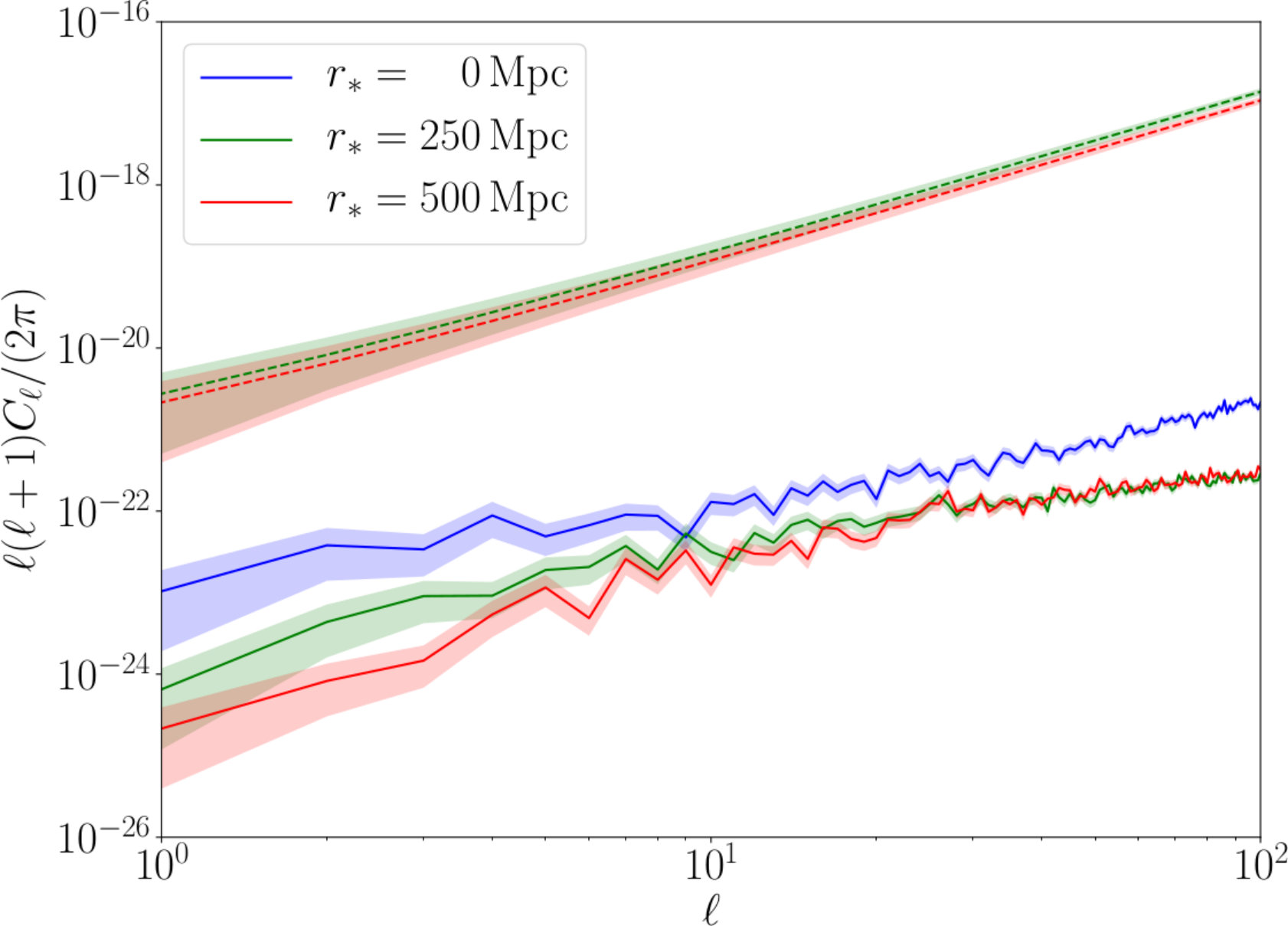 Figure 1
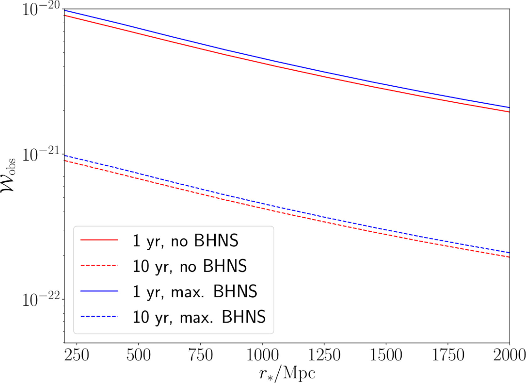 Figure 2
Peer Reviews
No public reviews on file for this paper yet. If you reviewed it on a platform where reviews are public (OpenReview, ICLR, NeurIPS, ICML), you can paste yours below so the community can read it here.
Videos
No videos yet. Explain this paper in a talk, walkthrough, or lecture? Add one.
Shot noise in the astrophysical gravitational-wave background
Alexander C. Jenkins
Theoretical Particle Physics and Cosmology Group, Physics Department, King’s College London, University of London, Strand, London WC2R 2LS, United Kingdom
Mairi Sakellariadou
Theoretical Particle Physics and Cosmology Group, Physics Department, King’s College London, University of London, Strand, London WC2R 2LS, United Kingdom
(16th March 2024)
Abstract
We calculate the shot noise induced in the anisotropies of the astrophysical gravitational-wave background by finite sampling of both the galaxy distribution and the compact binary coalescence event rate. This leads to a white noise term in the angular power spectrum , for which we derive a simple analytical expression. Failing to account for this term (as previous analyses have done) biases any measurement of the ’s. We find that the shot noise dominates over the true astrophysical power spectrum in any reasonable observing scenario, and that only with very long observing times and removal of a large number of foreground sources can the true power spectrum be recovered.
††preprint: KCL-PH-TH/2019-15
I Introduction
The Advanced LIGO Aasi et al. (2015) and Advanced Virgo Acernese et al. (2015) interferometers have instigated an exciting new era of astronomy by directly detecting gravitational waves (GWs). Eleven detections have been announced thus far Abbott et al. (2018a), each associated with a compact binary coalescence (CBC). However, aside from individual loud events like these, one expects a population of many CBCs that are too faint or numerous to be directly resolvable. The superposition of GWs from these events leads to the astrophysical gravitational-wave background (AGWB), a persistent GW signal that can be distinguished from instrumental noise by cross-correlating data from multiple detectors Romano and Cornish (2017); Smith and Thrane (2018). The AGWB is a vitally important target for GW observations, and is potentially detectable by LIGO and Virgo at design sensitivity Abbott et al. (2018b).
In the literature, the AGWB is often treated as perfectly isotropic, for simplicity. However, several recent studies Jenkins and Sakellariadou (2018); Jenkins et al. (2018a, b); Cusin et al. (2018) have investigated how the anisotropic distribution of GW sources and the inhomogeneous geometry of the spacetime through which the GWs propagate can induce anisotropies in the AGWB. By carefully studying these anisotropies, one can hope to use the AGWB as a probe of the large-scale structure (LSS) of the Universe, in particular, the distribution of galaxies on large angular scales.
The AGWB anisotropies calculated in Refs. Jenkins and Sakellariadou (2018); Jenkins et al. (2018a, b); Cusin et al. (2018) are expressed in terms of the angular power spectrum components . These are statistical quantities, describing the expected angular correlation of the AGWB after averaging the signal in at least three distinct ways: () averaging over random realisations of the cosmic matter distribution (“ensemble of Universes”), () averaging over the discrete positions of galaxies within the matter distribution to give a continuous galaxy number density field, and () averaging over the merger times of CBCs within each galaxy to give a mean merger rate. However, the AGWB we observe corresponds to a single Universe, with some discrete number of galaxies, each with some discrete number of CBCs. In practice, therefore, we are unable to perform the averaging process described above, leading to random fluctuations in the observed ’s, which must be accounted for when comparing to theoretical predictions. What is more, our most accurate theoretical predictions are themselves based on a simulated galaxy catalogue with a single realisation of LSS and a finite number of galaxies Jenkins et al. (2018a, b), so it is doubly important to understand these effects.
References Jenkins and Sakellariadou (2018); Jenkins et al. (2018a, b) have already accounted for point () above: the uncertainty due to our observation of a single realisation of LSS, i.e., cosmic variance. If the AGWB is Gaussian, then we have the standard result, . Besides cosmic variance, we must account for the fact that the AGWB is emitted from a finite number of galaxies (sampled from the underlying density field), each hosting a finite number of CBCs (sampled from the mean merger rate). These two sampling processes, corresponding to points () and () above, follow Poisson statistics and introduce shot noise to the observed angular power spectrum. This is a very important effect, which has been studied for decades in contexts such as galaxy redshift surveys Feldman et al. (1994); Hamilton (2008) and the cosmic infrared background Kashlinsky et al. (2018). In the context of the AGWB, Ref. Meacher et al. (2014) used numerical simulations to study the effects of shot noise on the monopole (i.e. isotropic component), but until now the effects of shot noise on the AGWB anisotropies have been ignored.
In this work, we derive expressions for the AGWB angular power spectrum in the presence of shot noise, and calculate the size of the shot-noise effects for realistic models of the AGWB in the LIGO/Virgo frequency band. We begin with a short description of our model of the AGWB, before defining the angular power spectrum components , and showing how they are affected by the presence of shot noise. We then derive an expression for this effect in terms of the CBC population and galaxy distribution, and show how the removal of nearby sources can mitigate it somewhat. We conclude by discussing the implications of our results for future GW observing runs.
II Modelling the AGWB
Here we briefly recap our model of the AGWB and its anisotropies, first presented in Ref. Jenkins et al. (2018a). We describe the AGWB in terms of its density parameter (in units where ),
[TABLE]
which is the energy density of GWs arriving at the observer from direction , with observer-frame frequency in a logarithmic bin centred on , normalised with respect to the critical density of the Universe, . We treat this as a random field on the sphere, whose angular statistics we wish to study.
The model in Ref. Jenkins et al. (2018a) writes the GW density field as an integral over the population of CBC sources,
[TABLE]
where is the Hubble time, is the redshift, is the dimensionless Hubble rate, is the set of parameters describing the galaxies and the CBCs, is the number density of galaxies with parameter values at position , is the rate of CBCs per galaxy as a function of redshift, and encodes the GW emission of each CBC as a function of source-frame frequency , as given by hybrid waveform models that are calibrated to numerical relativity simulations Ajith et al. (2008, 2011).
We calculate the rate function by convolving the star formation rate of each galaxy with a distribution of delay times (i.e. the interval between the time of star formation and the coalescence time for a given binary) and normalising to match the local CBC rates inferred by the LIGO/Virgo detections Abbott et al. (2018a). (This calculation also accounts for the suppression of high-mass black hole formation in high-metallicity environments.) The galaxy number density is given by a mock galaxy catalogue based on the Millennium Simulation Blaizot et al. (2005); De Lucia and Blaizot (2007); Springel et al. (2005); Lemson (2006). This allows us to create a simulated map of the AGWB by individually computing the contribution of each galaxy in the catalogue. The statistics of this map are then analysed with HEALPix Gorski et al. (2005).111http://healpix.sourceforge.net
III The angular power spectrum, with and without shot noise
We now show how the inclusion of generic shot-noise effects in the underlying statistics of the AGWB leads to an additional term in the angular power spectrum. For later convenience, we write as an integral over comoving distance,
[TABLE]
where is the Hubble radius, and we have defined a new dimensionless function . Comparing with Eq. (2), we see that
[TABLE]
(We suppress the frequency dependence from now on.)
We characterise the anisotropies of in terms of a multipole expansion of its covariance,
[TABLE]
which we call the angular power spectrum.222Note that we do not normalise with respect to the monopole as we did in Refs. Jenkins and Sakellariadou (2018); Jenkins et al. (2018a, b). This is because the monopole is now itself a random variable, and accounting for the variance due to this random normalisation would complicate things. The physical content of the definition Eq. (5) is the same as before. Here runs over all non-negative integers, and are the corresponding Legendre polynomials. Note that the ’s are independent of due to statistical isotropy. We can also write Eq. (5) as
[TABLE]
where we have decomposed the field into spherical harmonics,
[TABLE]
Equation (6) shows that each is an uncorrelated complex random variable with variance .
III.1 The ’s without shot noise
We calculate the angular power spectrum by specifying the second moment of the field. Neglecting shot noise, this is simply
[TABLE]
where is the two-point correlation function of , describing the probability in excess of random of similar values of the field being clustered together. Due to statistical isotropy, only depends on the angular positions of the two points through their separation . (It does, however, depend on their radial distances, as these influence the intensity of the GW flux.) Using Eqs. (3), (5), and (8), we find the ’s in the absence of shot noise,
[TABLE]
III.2 The ’s with shot noise
We now introduce a shot-noise term that encompasses both the galaxy sampling and the CBC rate sampling. Assuming these effects can jointly be treated as a local Poisson process that is independent of LSS, we have
[TABLE]
where is some function describing the variance due to the finite sample, which is independent of direction due to statistical isotropy. The factor of ensures that is dimensionless.
The form of this new shot-noise term [in particular, the fact that it is proportional to ], is motivated by the equivalent expression for galaxy surveys (see Appendix A of Ref. Feldman et al. (1994), or Sec. 2.4 of Ref. Hamilton (2008)). It is quite simple to convince oneself that the modification due to shot noise should take this form: there should be an extra term added to the covariance, as shot-noise fluctuations increase the variations in the measured values of throughout space, above the intrinsic variance due to the clustering of GW sources. However, since the shot-noise fluctuations at one point in space are causally disconnected from those at any other point, the fluctuations at any two points are statistically independent, and the extra term in the covariance should vanish except when the two points are coincident, leading to the delta function. Equation (10) thus arises naturally from the superposition of independent Poisson processes at each point in space. We flesh this argument out more quantitatively in Sec. IV.
Using Eqs. (3), (5), (9), and (10), as well as the fact that for all , the full angular power spectrum is then
[TABLE]
Thus we see that the shot noise generates a spectrally white (i.e., independent of ) contribution to the ’s.
IV Calculating the shot-noise power
In order to evaluate Eq. (11), we must derive an expression for the local Poisson variance function , accounting for the random sampling of both the galaxy number density and the CBC event rate.
Consider a volume element at position . We treat the number of galaxies in this region as a Poisson random variable, .333We stress that this is only an approximation. A more sophisticated approach would use the halo model of LSS Cooray and Sheth (2002), accounting for the statistical properties of dark matter halos and of different populations of galaxies within them. However, this approximation is sufficiently accurate for our purposes (particularly as the galaxy-number contribution to the shot noise is much less than the CBC rate contribution—see below). Assuming for now that these galaxies and the CBCs in them all have the same parameter values , the CBC event counts for each galaxy in a given source-frame time interval are independent and identically distributed Poisson random variables, . The total CBC event count from is then , which follows a compound Poisson distribution with variance
[TABLE]
(This can be shown by computing the moment generating function of .) Taking the sampling as independent for different spatial volumes and for different parameter values, we find
[TABLE]
where we have averaged over LSS so that . Replacing with the comoving CBC rate density, , and taking , we are left with
[TABLE]
where is shorthand for , etc. The relationship between the source-frame time and the observer-frame time will generally depend on cosmological metric perturbations and peculiar velocities at the location of the source, but to leading order it is simply .
Using Eqs. (4) and (10), the shot-noise power is therefore
[TABLE]
Equation (15) is our main result, and has two distinct applications: () interpreting future observations of the AGWB, and () improving our theoretical models. For the former, we can use Eq. (15) to calculate the expected shot noise in the observed spectrum as a function of observing time, given a model for the galaxy number density and CBC merger rate. The term dominates over the term, as for a typical galaxy. For the latter, we can use Eq. (15) to calculate the error inherent to our theoretical predictions, due to the finite galaxy sampling in the simulated galaxy catalogue Jenkins et al. (2018a, b). Since these predictions do not involve simulating the time of arrival of discrete GW signals, but average over the CBC rate, they exclude the shot noise due to sampling of this rate. This is identical to taking the limit , meaning that the catalogue predictions contain shot noise due to the term only. We therefore distinguish between the “observational shot noise” and the “catalogue shot noise,”
[TABLE]
Here, represents the galaxy number density in the catalogue, which is significantly less than the true galaxy number density (this is because only galaxies brighter than a certain magnitude are included). Expressing this as a weighted sum of delta functions, with each term representing a single galaxy, the catalogue shot noise is approximated by
[TABLE]
V Removing the foreground
Inspecting Eq. (15), we see that the integrand diverges as . This is to be expected, for two reasons. First, the Poisson statistics become progressively worse at small distances, as we are looking at smaller spherical shells that contain fewer galaxies, so the notion of a smooth number density breaks down as . Second, the contribution of a single CBC to the total AGWB flux becomes much larger at smaller distances, so a CBC that is arbitrarily close can bias the power spectrum by an arbitrarily large amount.
In order to regulate this divergence, it is necessary to introduce a cutoff distance , below which we remove any CBC signals and do not consider them part of the AGWB. (This is similar to what is done with, e.g., the cosmic infrared background Kashlinsky et al. (2018).) We are free to choose the value of , with larger values helping to reduce the shot noise as much as possible. However, the choice of will also affect , and this must be accounted for when making theoretical predictions.
In principle, one can implement this foreground cut by removing from the GW strain time series any intervals in which an individual CBC with a comoving distance is identified. The CBC chirp signal encodes the luminosity distance , which can easily be converted to the comoving distance by assuming a fiducial cosmology. However, cannot be measured with arbitrary precision, particularly as it is degenerate with the inclination of the binary. What is more, the detectability of CBCs at a given distance is also a function of sky position, due to the anisotropic beam pattern of the detectors. Removing nearby sources based on a signal-to-noise threshold (as in Ref. Meacher et al. (2014)) risks biasing the power spectrum by favouring particular kinds of CBC events and particular regions of the sky. It is therefore crucial that is set to be small enough that all CBCs at distances are detectable, so the foreground removal can be implemented in an unbiased and isotropic manner, without selection effects. It may be desirable to set different cutoffs for different sources; e.g., a much larger value for binary black holes than for binary neutron stars, as the former are detectable at much larger distances. We leave a detailed examination of these practical issues for future work Jenkins et al. .
VI Discussion and conclusion
Using the AGWB model Jenkins et al. (2018a, b) described above, we can calculate the size of the observational and catalogue shot-noise terms from Eq. (16) for different values of the foreground cutoff distance . We find that the catalogue shot noise is for , and is typically several orders of magnitude smaller than this for . Since the monopole is , this represents shot-noise fluctuations of . This is negligible compared to the true power spectrum , so our earlier predictions in Refs. Jenkins et al. (2018a, b) are completely unaffected.444In particular, we emphasise that the catalogue shot noise cannot explain why the angular power spectrum calculated in Refs. Jenkins et al. (2018a, b) is more than an order of magnitude larger than that in Ref. Cusin et al. (2018): the predicted spectrum is all but identical once the catalogue shot noise is subtracted. We refer the reader to Refs. Jenkins et al. (2018a, b, 2019) for discussion of the likely causes of this discrepancy.
On the other hand, we find that the observational shot noise is generically several orders of magnitude larger than the true angular power spectrum for any reasonable values of and . (In fact, , so the shot-noise fluctuations are typically as large as the monopole itself.) This is illustrated in the right-hand panel of Fig. 1 for and . Note that also changes with , partly because the total GW emission is reduced, causing an overall reduction in the spectrum, and partly because the nearest galaxies contribute most strongly to the AGWB, so that their removal changes the shape of the spectrum. Calculations of using the catalogue are not reliable for values of significantly larger than , due to the incompleteness of the catalogue at high redshift. However, as can be seen in the left-hand panel of Fig. 1, even increasing from to can only reduce by less than an order of magnitude, so this seems unlikely to solve the problem.
The numerical values given in Fig. 1 depend on the details of the AGWB model, and include a multitude of random and systematic uncertainties in, e.g., the populations of astrophysical sources that contribute, their emission rates, and the nature of their clustering. However, we stress that the main result, Eq. (11), is generic, and is grounded in simple and realistic physical principles. Any finite population of sources will have random Poissonian fluctuations. If these fluctuations are statistically independent at different spatial locations (i.e., if the shot-noise fluctuations are causally disconnected), then the angular power spectrum generically gains an extra white-noise component, . If these sources are finite in time, then basic Poisson statistics dictates that this noise decays as the inverse of the observation time, .
These results raise the question of whether it is possible to mitigate the shot noise, and thereby probe on reasonable observational timescales. In the context of galaxy redshift surveys, there are a range of statistical methods for suppressing the effects of shot noise, many of which involve applying some optimal weighting to each galaxy, such as the “FKP weighting” Feldman et al. (1994); Hamilton (2008). Could similar methods be developed for the AGWB? The fundamental issue with this idea is that the AGWB consists primarily of unresolved events, and it is therefore not clear how any kind of weighting could be applied in practice. Note however that in the era of third-generation GW detectors such as the Einstein Telescope Punturo et al. (2010), almost every binary black hole coalescence in the observable Universe will be resolvable Regimbau et al. (2017), and it may become possible to study LSS with optimally weighted CBC number counts. Another possibility is to study the cross correlation of the AGWB with electromagnetic (EM) probes of LSS (e.g. galaxy surveys, or weak lensing). Since these EM observables have a lower level of shot noise, one would naively expect the shot noise of the cross-correlated spectrum to be smaller than for the AGWB autocorrelation studied here. This cross-correlated spectrum could be used to test for the presence of primordial black holes in the AGWB, using a similar approach to Ref. Scelfo et al. (2018).
The results presented here are of vital importance for interpreting future observations of the AGWB. They show that it will be much harder than previously thought to uncover the cosmological information encoded in the AGWB anisotropies. Nonetheless, it remains possible that with sufficient foreground subtraction, and with long enough observing runs, this information might still be accessible by LIGO and Virgo at design sensitivity, or by third-generation GW detectors such as the Einstein Telescope Punturo et al. (2010). This is an important open question that warrants further investigation.
Acknowledgements.
We thank Vuk Mandic for helpful comments on the manuscript, and for insightful discussions on related issues. This work has been assigned the document number LIGO-P1900050. The Millennium Simulation databases used in this work and the web application providing online access to them were constructed as part of the activities of the German Astrophysical Virtual Observatory. Some of the results in this work have been derived using the HEALPix package Gorski et al. (2005). A.C.J. is supported by King’s College London through a Graduate Teaching Scholarship. M.S. is supported in part by the Science and Technology Facility Council (STFC), United Kingdom, under the research grant No. ST/P000258/1.
The reference list from the paper itself. Each links out to its DOI / PubMed record.
- 1Aasi et al. (2015) J. Aasi et al. (LIGO Scientific), “Advanced LIGO,” Class. Quant. Grav. 32 , 074001 (2015) , ar Xiv:1411.4547 [gr-qc] . · doi ↗
- 2Acernese et al. (2015) F. Acernese et al. (Virgo), “Advanced Virgo: a second-generation interferometric gravitational wave detector,” Class. Quant. Grav. 32 , 024001 (2015) , ar Xiv:1408.3978 [gr-qc] . · doi ↗
- 3Abbott et al. (2018 a) B. P. Abbott et al. (LIGO Scientific, Virgo), “GWTC-1: A Gravitational-Wave Transient Catalog of Compact Binary Mergers Observed by LIGO and Virgo during the First and Second Observing Runs,” (2018 a), ar Xiv:1811.12907 [astro-ph.HE] .
- 4Romano and Cornish (2017) Joseph D. Romano and Neil J. Cornish, “Detection methods for stochastic gravitational-wave backgrounds: a unified treatment,” Living Rev. Rel. 20 , 2 (2017) , ar Xiv:1608.06889 [gr-qc] . · doi ↗
- 5Smith and Thrane (2018) Rory Smith and Eric Thrane, “Optimal Search for an Astrophysical Gravitational-Wave Background,” Phys. Rev. X 8 , 021019 (2018) , ar Xiv:1712.00688 [gr-qc] . · doi ↗
- 6Abbott et al. (2018 b) Benjamin P. Abbott et al. (LIGO Scientific, Virgo), “GW 170817: Implications for the Stochastic Gravitational-Wave Background from Compact Binary Coalescences,” Phys. Rev. Lett. 120 , 091101 (2018 b) , ar Xiv:1710.05837 [gr-qc] . · doi ↗
- 7Jenkins and Sakellariadou (2018) Alexander C. Jenkins and Mairi Sakellariadou, “Anisotropies in the stochastic gravitational-wave background: Formalism and the cosmic string case,” Phys. Rev. D 98 , 063509 (2018) , ar Xiv:1802.06046 [astro-ph.CO] . · doi ↗
- 8Jenkins et al. (2018 a) Alexander C. Jenkins, Mairi Sakellariadou, Tania Regimbau, and Eric Slezak, “Anisotropies in the astrophysical gravitational-wave background: Predictions for the detection of compact binaries by LIGO and Virgo,” Phys. Rev. D 98 , 063501 (2018 a) , ar Xiv:1806.01718 [astro-ph.CO] . · doi ↗