
TL;DR
This paper proves that every quasiconformal tree can be transformed into a geodesic tree with Hausdorff dimension close to 1 using quasisymmetric mappings, linking these classes of metric trees.
Contribution
It establishes a quasisymmetric equivalence between quasiconformal trees and geodesic trees with nearly one-dimensional Hausdorff measure.
Findings
Quasiconformal trees are quasisymmetrically equivalent to geodesic trees.
The Hausdorff dimension of these geodesic trees can be made arbitrarily close to 1.
The result connects the geometric structure of quasiconformal trees to geodesic trees.
Abstract
A quasiconformal tree is a metric tree that is doubling and of bounded turning. We prove that every quasiconformal tree is quasisymmetrically equivalent to a geodesic tree with Hausdorff dimension arbitrarily close to 1.
Click any figure to enlarge with its caption.
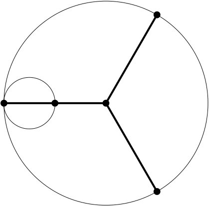 Figure 1
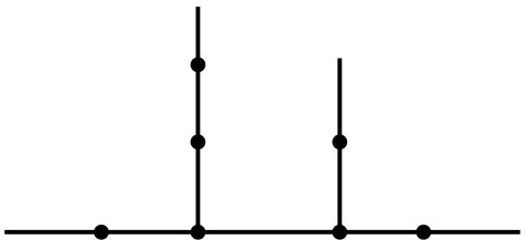 Figure 2
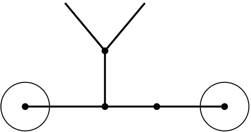 Figure 3
 Figure 4
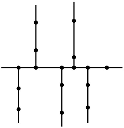 Figure 5
 Figure 6
Peer Reviews
No public reviews on file for this paper yet. If you reviewed it on a platform where reviews are public (OpenReview, ICLR, NeurIPS, ICML), you can paste yours below so the community can read it here.
Videos
No videos yet. Explain this paper in a talk, walkthrough, or lecture? Add one.
Quasiconformal and geodesic trees
Mario Bonk
Department of Mathematics, University of California, Los Angeles, CA 90095, USA
and
Daniel Meyer
Department of Mathematical Sciences, University of Liverpool, Liverpool L69 7ZL, United Kingdom
Abstract.
A quasiconformal tree is a metric tree that is doubling and of bounded turning. We prove that every quasiconformal tree is quasisymmetrically equivalent to a geodesic tree with Hausdorff dimension arbitrarily close to 1.
Key words and phrases:
Quasiconformal tree, geodesic tree, quasisymmetry, doubling metric spaces, bounded turning, conformal dimension
2010 Mathematics Subject Classification:
Primary 30L10; Secondary 51F99
Contents
1. Introduction
An important question in geometric analysis is whether a given metric space (belonging to some class of spaces) is geometrically equivalent to a model space in a natural way. Many results in mathematics can be seen from this perspective (such as the existence of isothermal or conformal coordinates on surfaces or the Riemann mapping theorem). For general metric spaces there are various ways to interpret geometric equivalence: up to isometric or up to bi-Lipschitz equivalence, for example. In the present paper the relevant notion of geometric equivalence is based on a class of homeomorphisms that are close to conformal or quasiconformal maps in a classical complex-analytic context, namely quasisymmetries.
By definition, a homeomorphism between metric spaces and is said to be quasisymmetric or a quasisymmetry, if there exists a homeomorphism (playing the role of a control function for distortion) such that
[TABLE]
for all distinct points . The composition of two quasisymmetries (when defined) and the inverse of a quasisymmetry are quasisymmetric. So if we call two metric spaces and quasisymmetrically equivalent if there exists a quasisymmetry , then we have a notion of geometric equivalence for metric spaces. Since every bi-Lipschitz homeomorphism is a quasisymmetry, this is a weaker, and hence more flexible, notion than bi-Lipschitz (or even isometric) equivalence (for more background and related discussions see [BM17, Section 4.1] and [He01, Chapters 10–12]).
The quasisymmetric uniformization problem (see [Bo06]) asks for natural conditions when a given metric space from a class of spaces is quasisymmetrically equivalent to some model space . This problem is relevant in various contexts. For example, the Kapovich-Kleiner conjecture in geometric group theory (see [KK00, Conjecture 6]) amounts to the problem of showing that every Sierpiński carpet arising as the boundary of a Gromov hyperbolic group is quasisymmetrically equivalent to a “round” Sierpiński carpet (see [Bo11] for a related discussion).
The prototypical instance of a quasisymmetric uniformization result is the characterization by Tukia and Väisälä of metric spaces quasisymmetrically equivalent to the unit interval . In order to formulate their theorem we need two definitions.
We say that a metric space is of bounded turning if there exists a constant such that for all there exists a compact connected set with and
[TABLE]
In this case, we say that is of -bounded turning.
A metric space is doubling if there exists a constant (the doubling constant of ) such that each ball in of radius can be covered by (or fewer) balls of radius .
Tukia and Väisälä showed that a metric space homeomorphic to is quasisymmetrically equivalent to if and only if it is doubling and of bounded turning (see [TV80]). In other words, one can “straighten out” the arc (which may well have Hausdorff dimension ) to the interval by a quasisymmetry.
In the present paper, we study the quasisymmetric uniformization problem for metric trees. By definition, a (metric) tree is a compact, connected, and locally connected metric space that contains at least two distinct points and has the following property: if , then there exists a unique arc in with endpoints and . This arc is denoted by . We allow here, in which case we consider as a degenerate arc.
The underlying topological space of a tree is often called a dendrite in the literature. Since we are mostly interested in metric properties and want to emphasize this metric aspect, we prefer the name tree for these objects. Motivated by the Tukia-Väisälä result and the connection with quasiconformal geometry, we introduce the following terminology.
Definition 1.1**.**
A metric tree is quasiconformal if it is doubling and of bounded turning.
In the following, we usually call a quasiconformal tree a qc-tree for brevity.
Trees appear in many contexts in mathematics, for example as Julia sets of polynomials. The Julia set of the polynomial is a tree (see [CG93, Example after Theorem V.4.2]). Actually, is a qc-tree if it is equipped with the ambient Euclidean metric on . Indeed, is of bounded turning as easily follows from the fact that is a John domain (see [CG93, Theorem VII.3.1]). Since every subset of a Euclidean space (such as the complex plane ) is doubling, is doubling.
In analogy to the Tukia-Väisälä theorem one can raise the question whether all arcs in a qc-tree can be straightened out simultaneously by a quasisymmetry. For a precise formulation of this question the following concept is relevant.
A metric space is called geodesic if any two points can be joined by a geodesic segment, i.e., by an arc with endpoints and whose length is equal to .
The following statement is the main result of this paper.
Theorem 1.2**.**
Every quasiconformal tree is quasisymmetrically equivalent to a geodesic tree.
Every arc that is doubling and of bounded turning is a qc-tree. This implies that Theorem 1.2 includes the Tukia-Väisälä theorem as a special case, and so can it be viewed as a generalization.
Various improvements and variants of Theorem 1.2 are conceivable. For example, one can ask whether additional assumptions yield quasisymmetric equivalence to a single specified space. We consider a question of this type in the follow-up paper [BM20], where it is shown that a qc-tree is quasisymmetrically equivalent to the continuum self-similar tree (as defined in [BT20]) if and only if it is trivalent and uniformly branching (see [BM20] for the relevant definitions).
Another natural question is “how small” we can make the geodesic tree that is the quasisymmetric image of the given qc-tree . If denotes the Hausdorff dimension of , then clearly , because always contains a non-degenerate arc. We will show that can actually be arbitrarily close to and will establish the following improved version of Theorem 1.2.
Theorem 1.3**.**
If is a quasiconconformal tree and , then is quasisymmetrically equivalent to a geodesic tree with .
In general, one cannot achieve here. An example when this is not possible can be found in [BiT01] (see also [Az15, Theorem 1.6] for a general related statement). If is the continuum self-similar tree and is any tree that is quasisymmetrically equivalent to , then actually .
The conformal dimension of a metric space is defined as the infimum of all Hausdorff dimensions of metric spaces that are quasisymmetrically equivalent to . We refer to [MT10] for more background on this concept. Theorem 1.3 implies the following immediate consequence.
Corollary 1.4**.**
If is a quasiconformal tree, then .
This last statement is not new, but was originally proved by Kinneberg [Kin17, Proposition 2.4].
We will now summarize the main ingredients for the proofs of Theorems 1.2 and 1.3. The basic idea is to define a new geodesic metric on the given qc-tree so that the identity map is a quasisymmetry. In order to define , we will carefully choose a sequence of decompositions of into subtrees. We call the elements in tiles of level or -tiles. To each -tile we will assign a weight by an inductive process on the level . These weights can then be used to define a distance function on : one infimizes the total length with respect to this weight over chains of -tiles from one point in to another (see (6.1) and (7.1)). We will show that with our choices, the limit
[TABLE]
exists for all (Lemma 7.3) and defines a geodesic metric on (Lemma 7.6). We have for the -diameter of each tile (see Proposition 7.7 (i)). So in a sense the metric is a “conformal” deformation of the original metric on controlled by the weight near each tile . The fact that is a quasisymmetry can then easily be derived from geometric properties of tiles (see Lemma 8.2). Theorem 1.2 follows.
The choice of the weights and hence the construction of involves a parameter . We will see that if we choose close to [math], then the Hausdorff dimension of is close to . This immediately gives Theorem 1.3.
The main difficulty in this general approach is how to define the decompositions . It is a natural idea to “cut” the tree into subtrees by using auxiliary points. We will indeed follow this procedure by defining an ascending sequence of finite sets that we use to cut . More precisely, the tiles of level are precisely the closures of the complementary components of , i.e., the closures of the components of . The construction of the sets involves a (small) parameter . For each -tile we will then have . All of this looks natural and even straightforward, but there is a surprising subtlety here. Namely, one might expect that the -vertices, i.e., the elements in used for cutting the tree, should be branch points of (points such that has at least three components); indeed, at least on an intuitive level, cutting in a branch point should result in branches with reduced topological or metric complexity. This was exactly the procedure in the recent paper [BT20], where topological characterizations of metric trees were given. We also use this idea in our forthcoming paper [BM20]. However, in the present context, cutting our given qc-tree at a branch point leads to the problem that we cannot expect good uniform control for the size of the components of , because some of these components might be very small.
For this reason, we cut our given qc-tree at double points , i.e., points such that has precisely two components. These double points are chosen so that the two components of are not too small and so that stays away from the branch points of in a precise quantitative way (see (4.1) and (4.2); the relevant definitions can be found in (2.1) and (2.2)).
The paper is organized as follows. In Section 2 we review some basic topological facts about trees. We also show that in a tree of bounded turning one can replace the original metric up to bi-Lipschitz equivalence by a diameter metric . It is characterized by the property that for all . The change to a diameter metric will allow us to make some simplifications of our arguments. In Section 3 we will prove a general fact of independent interest: if on an arc some points cast a “shadow” satisfying suitable conditions, then one can always find a “place in the sun”. We use this to find double points in a qc-tree with quantitative separation from branch points (see Proposition 3.1).
In Section 4 we introduce the somewhat technical concept of a -good double point at scale . We show that with suitable choices of the parameters cutting the qc-tree in a maximal -separated set of -good double points at scale results in pieces that have diameter comparable to (Proposition 4.2). This fact is used in Section 5 to define the subdivisions of into tiles as discussed above. We record various statements about the geometric properties of these tile decompositions. Weights of tiles are then defined in Section 6. There we establish the facts about weights that are needed later on. In Section 7 we define the metric and show that it is geodesic. The proof of Theorem 1.2 is then completed in Section 8 and the proof of Theorem 1.3 is given in Section 9. We conclude with remarks and open problems in Section 10.
1.1. Notation
We summarize some notation used throughout this paper.
When an object is defined to be another object , we write for emphasis. Two non-negative quantities and are said to be comparable if there is a constant (usually depending on some ambient parameters) such that
[TABLE]
We then write . The constant is referred to as . Similarly, we write or , if there is a constant such that , and refer to the constant as or . If we want to emphasize the parameters , on which depends, then we write .
We use the standard notation and .
The cardinality of a set is denoted by and the identity map on by . Let be a metric space, , and . We denote by the open ball and by \makebox[0.0pt]{\phantom{B}\overline{\phantom{B}}}B_{d}(a,r)=\{x\in X:d(a,x)\leq r\} the closed ball of radius centered at . If , we let be the diameter, be the closure of in , be the interior of in , and
[TABLE]
be the distance of and . If , we set . We drop the subscript from our notation for , etc., if the metric is clear from the context.
2. Auxiliary facts
In this section we collect some auxiliary statements that will be used later.
Let be a metric space. A set is called -separated for some if all distinct points satisfy . Such a set is a maximal -separated set if is not contained in a strictly larger subset of that is also -separated. Every -separated set is contained in a maximal -separated set . If is compact, then every -separated set must be finite.
If the space is doubling (as defined in the introduction), then for each there is a number only depending on and the doubling constant of such that the following condition is true: if and is a -separated set contained in a ball with , then contains at most points. Conversely, if this condition is true for some and , then is doubling with a doubling constant only depending on and (see [He01, Exercise 10.17]).
The doubling property is preserved under quasisymmetries, and in particular under bi-Lipschitz maps; in general though, the doubling constant will change (see [He01, Theorem 10.18]).
An arc is a set homeomorphic to the unit interval . A (metric) arc is a metric space homeomorphic to . The points corresponding to are called the endpoints of . We denote by the set of endpoints of , and by the set of interior points of .
We require an elementary lemma.
Lemma 2.1**.**
Let be an arc and be an integer. Then we can decompose into non-overlapping subarcs of equal diameter .
More explicitly, decomposing into non-overlapping subarcs means that we can find arcs with pairwise disjoint interiors such .
Proof.
The existence of a decomposition of into non-overlapping subarcs of equal diameter is proved in [Me11, Lemma 2.2] (see also [Kul94, Lemma 2] for a related statement in greater generality). If we denote this diameter by , then we must have as follows from the triangle inequality. ∎
We now summarize some simple facts about trees. There is a rich literature on the underlying topological spaces, usually called dendrites. We refer to [Wh63, Chapter V], [Kur68, Section §51 VI], [Na92, Chapter X], and the references in these sources for more on the subject.
By definition, a metrizable topological space is called a dendrite if is a Peano continuum (i.e., it is compact, connected, and locally connected), and does not contain any Jordan curve (i.e., a homeomorphic image of the unit circle). A dendrite is called non-degenerate if it contains more than one point. The following statement reconciles our notion of a metric tree with the notion of a dendrite.
Proposition 2.2**.**
Let be a metric space. Then is a tree if and only if is a non-degenerate dendrite.
Proof.
“” If is a tree, then it is a Peano continuum and contains more than one point. Moreover, cannot contain a Jordan curve . Indeed, if contains the Jordan curve , then any two distinct points can be connected by at least two distinct arcs in , namely the two subarcs of with endpoints and . This is impossible, because is a tree. It follows that is a non-degenerate dendrite.
“” Conversely, suppose is a non-degenerate dendrite. Since is a Peano continuum, it is arc-connected, i.e., for any two distinct points there exists an arc with endpoints and (see [Na92, Theorem 8.23]). This arc is unique, because if there exists an arc with and endpoints and , then it is easy to see that contains a Jordan curve. This is impossible, because is a dendrite. It follows that is indeed a tree. ∎
Let be a tree. Then for all points with , there exists a unique arc in joining and , i.e., it has the endpoints and . We use the notation for this unique arc. It is convenient to allow here. Then denotes a degenerate arc consisting only of the point . Sometimes we want to remove one or both endpoints from the arc . Accordingly, we define
[TABLE]
If is the image of any path in joining and , then necessarily .
A subset of a tree is called a subtree of if equipped with the restriction of the metric is also a tree. One can show that is a subtree of if and only if contains at least two points and is closed and connected. See [BT20, Lemma 3.3] for a simple direct argument; to justify this, one can also invoke Proposition 2.2 and the fact that a closed and connected subset of a dendrite is a dendrite (see [Na92, Corollary 10.6]). If is a subtree of , then for all .
Lemma 2.3**.**
Let be a tree and be a finite set. Then the following statements are true:
- (i)
Two points lie in the same component of if and only if . 2. (ii)
If is a component of , then is an open set and is a subtree of with . 3. (iii)
If and and are distinct components of , then and have at most one point in common. Such a common point belongs to , and is a boundary point of both and .
Proof.
(i) Since is a finite set, it is closed in . So is an open subset of . Since is locally connected, each component of is open. Moreover, as an open and connected subset of the Peano continuum , such a component is arc-connected (see [Na92, Theorem 8.26]). So if two points lie in the same component of , then there exists an arc in joining and . Then , and so .
Conversely, if and , then is a connected subset of . Hence there exists a component of with ; so and lie in the same component of .
(ii) If is a component of , then is an open set (as we have seen in the proof of (i)) and is a subtree of (as follows from the characterization of subtrees discussed before the lemma).
The inclusion is true for all sets . It remains to show . Indeed, if , then cannot belong to (since is open) or any other component of (because otherwise ); so lies in the complement of in , i.e., .
(iii) Suppose and are distinct components of . Since and are disjoint open subsets of by (ii), no interior point of can belong to , and no interior point of can belong to . Hence
[TABLE]
by (ii). In particular, is a subset of the finite set , and any point in must be a boundary point of both and .
Actually, consists of at most one point; otherwise, contains two distinct points and , and hence the infinite set , because and are subtrees of . This is impossible, because the set is finite. ∎
Let be a tree, , and be a component of . Then is open, and so , because is connected. So by Lemma 2.3 (ii) we have . Hence and so . Then is a subtree of , called a branch of (in ).
The components of any open subset of a tree form a null sequence in the following sense: for each there are only finitely many such components with . In particular, the number of components of is finite or countably infinite. This follows from a more general fact about open subsets of hereditarily locally connected metric continua; see [Wh63, p. 90, Corollary (2.2)] or [Kur68, p. 269, Theorem 3]. Note that we can apply this result by Proposition 2.2 and because every dendrite is hereditarily locally connected (this is explicitly stated in [Na92, Corollary 10.5] and follows from the fact, mentioned above, that every subcontinuum of a dendrite is a dendrite).
In particular, each point in a tree can have at most countably many distinct complementary components and hence there are only countably many distinct branches of . Only finitely many of these branches can have a diameter exceeding a given positive number (for a direct proof of these facts see also [BT20, Section 3]). This implies that we can label the branches of by numbers so that
[TABLE]
If there are precisely two such branches, then we call a double point of and define
[TABLE]
So is the diameter of the smallest branch of a double point .
If there are at least three branches of , then is called a branch point of . In this case, we set
[TABLE]
So is the diameter of the third largest branch of .
The following statement gives a criterion how to detect branch points.
Lemma 2.4**.**
Let be a tree, with and suppose that the sets , , are pairwise disjoint. Then the points lie in different components of and is a branch point of .
Proof.
This is [BT20, Lemma 3.6]. For the reader’s convenience we reproduce the argument. The arcs and have only the point in common. So their union is an arc and this arc must be equal to . Hence which by Lemma 2.3 (i) implies that and lie in different components of . A similar argument shows that must be contained in a component of different from the components containing and . In particular, has at least three components and so is a branch point of . The statement follows. ∎
The tree is of -bounded turning with (as defined in the introduction) if and only if
[TABLE]
for all . Here and in the following, instead of denotes the diameter of the arc ; we omit the parentheses for better readability.
We define the diameter distance on by
[TABLE]
for . We record some properties of this distance function.
Lemma 2.5**.**
*Let be a metric tree. Then the following statements are true:
- (i)
* is a metric on .* 2. (ii)
For each arc we have
[TABLE]
where denotes the diameter with respect to . 3. (iii)
* is of -bounded turning.* 4. (iv)
* is of -bounded turning for if and only if the identity map is -bi-Lipschitz.*
Proof.
This is [Me11, Lemma 2.1], but we will include the simple proof for the convenience of the reader.
(i) All properties of a metric for are immediate except the triangle inequality which follows from the fact that if , then .
(ii) For all , we have , and so . Moreover, for all we have . Hence ; so and the statement follows.
(iii) This follows directly from (ii), since
[TABLE]
for all .
(iv) If is of -bounded turning, then for all we have
[TABLE]
Thus the identity map is -bi-Lipschitz. Conversely, if this map is -bi-Lipschitz, then for all ,
[TABLE]
Therefore, is of -bounded turning. ∎
We say a metric on a metric tree is a diameter metric if for all . In this case, , where is defined as in (2.3).
Suppose is a qc-tree, i.e., a tree that is doubling and of bounded turning. Then the previous lemma implies that is bi-Lipschitz equivalent, and in particular quasisymmetrically equivalent, to . Moreover, is of -bounded turning and also doubling, since the latter condition is invariant under bi-Lipschitz equivalence; so is also a qc-tree. This implies that in order to prove Theorems 1.2 and 1.3, we are reduced to the case that the qc-tree in question carries a diameter metric. This reduction makes the proofs somewhat easier, but we still face major problems, because there is no obvious way to turn a diameter metric into a geodesic metric by a quasisymmetry.
For the rest of the paper we will assume that is a qc-tree that is equipped with a diameter metric . Nothing essential changes if we rescale the metric. So we may also assume that . We will denote the doubling constant of by throughout the paper.
3. Sun and shadow
In this section we will prove a statement, Proposition 3.1, that will allow us to find double points in our given qc-tree that stay away from the branch points of in a geometrically controlled manner. In the formulation of the proposition, we use the function defined in (2.2).
Proposition 3.1**.**
There exists a constant only depending on the doubling constant of with the following property: if and is an arc with , then there exists a double point of such that
[TABLE]
for all branch points .
To prove this statement, we require two auxiliary facts.
Lemma 3.2**.**
Let be a metric arc equipped with a diameter metric , be an arc, and be a set with , where . Then there exists an arc such that
[TABLE]
The statement is somewhat technical, because three arcs are involved, but in this form the lemma will be useful for us later on.
Proof of Lemma 3.2.
The construction that follows is illustrated in Figure 1. By Lemma 2.1 we can decompose into non-overlapping arcs of equal diameter .
We have
[TABLE]
Since and have pairwise disjoint interiors, by the pigeon-hole principle there exists such that for we have We subdivide into three non-overlapping arcs of equal diameter. Then
[TABLE]
for . We may assume that contains one endpoint of , contains the other endpoint, and is the “middle” arc in the decomposition of . It easily follows from (3.1) and the intermediate value theorem that there exists an arc with .
If , then . So if we travel from a point to the point along , we must traverse or . Since is a diameter metric, (3.1) implies that
[TABLE]
Hence . The statement follows. ∎
Lemma 3.3** **(Ein Platz an der Sonne111Mit fünf Mark
sind Sie dabei!).
Let be a metric arc equipped with a diameter metric , and be a function. Suppose that there is a constant such that for all subarcs we have
[TABLE]
Then there exists a constant and a point such that for all .
In other words, the set is non-empty (here we use the convention that ). If we think of each point with as “casting a shadow” of radius around , then the lemma says that the union of all shadows does not cover , and so there is a “place in the sun”.
Proof.
Without loss of generality we may assume that . Consider the set . Let and define for . Obviously, for and . We will inductively define arcs for such that , for all , and for all .
We set . Suppose arcs with the desired properties have already been defined for some . Then by our hypotheses It follows from Lemma 3.2 that we can find an arc with
[TABLE]
and . Hence has the desired properties, and we can continue the process indefinitely.
We have , and so we can pick a point that lies in all arcs . If is arbitrary, then there exists a smallest such that . Then , and so
[TABLE]
So if we choose , then is a point as desired. ∎
Proof of Proposition 3.1.
Let and suppose is an arc with . Then , where are the endpoints of . We set for , for a branch point , and for all other points . Since and for , we can consider as a function .
Claim. There exists a constant such that for all arcs we have
[TABLE]
In other words, satisfies the hypotheses of Lemma 3.3 with a constant only depending on the doubling constant of .
To see this, fix an arc and let , where . Each point is a branch point of and there exists a large component of that is disjoint from , but attached to through the point . There are such components. The doubling property then gives a bound on only depending on . In the following we present the details of this argument, illustrated in Figure 2.
We have , where are the endpoints of . Consider an arbitrary point . Then is a branch point of with . Each of the connected sets and is contained in a component of . Hence there must be another component of with that is disjoint from . There exists a point with ; otherwise, \makebox[0.0pt]{\phantom{U}\overline{\phantom{U}}}U_{r}=U_{r}\cup\{r\}\subset B(r,\rho/2) and so \operatorname{diam}(U_{r})\leq\operatorname{diam}(\makebox[0.0pt]{\phantom{U}\overline{\phantom{U}}}U_{r})<\rho, which is a contradiction.
Then , and it easily follows from the intermediate value theorem that we can find a point with . We have
[TABLE]
and so .
If with , then the corresponding points and lie in different components of . To see this, note that \makebox[0.0pt]{\phantom{U}\overline{\phantom{U}}}U_{r}=U_{r}\cup\{r\} is a connected set with
[TABLE]
and so \makebox[0.0pt]{\phantom{U}\overline{\phantom{U}}}U_{r} is contained in a component of . In particular, and lie in the same component of . On the other hand, was chosen from a component of that does not contain any point of .
Since and lie in different components of , Lemma 2.3 (i) implies that . In particular,
[TABLE]
So the points , , have pairwise mutual distance and are all contained in the ball . It follows that is bounded by a constant only depending on (see the discussion in the beginning of Section 2). Since the endpoints of are not contained in , we have to possibly increase this bound by to obtain a bound as in (3.3) with a constant . The Claim follows.
Lemma 3.3 now guarantees the existence of a point such that
[TABLE]
for all , where can be chosen to depend only on and hence on . We may assume that , and so .
We claim that the statement of the proposition is true with which only depends on . To see this, let be an arbitrary branch point of . As we travel from to along the arc , there is a first point . We now consider two cases depending on the location of .
Case 1. . In this case, we may assume . Since , by choice of we then have
[TABLE]
This is the desired inequality in this case.
Case 2. . Then in particular . There exists a component of that is disjoint from and satisfies . This connected set does not contain and so it is contained in a component of . Hence
[TABLE]
Two other components and of contain the half-open (and non-empty) arcs and , respectively. The situation is illustrated in Figure 3. It follows that
[TABLE]
Here we have used that . Similarly, , and so
[TABLE]
It follows that
[TABLE]
as desired.
Note that is a double point of . Indeed, is not a branch point of , because has a positive distance to each of them. On the other hand, , and so . Similarly, . Since , the points and lie in different components of by Lemma 2.3 (i). In particular, there are at least two, but not more than two such components. Hence is a double point of . ∎
With some small changes in the previous proof one can show that the set of double points that satisfy the estimate in Proposition 3.1 is not only non-empty, but in a suitable sense actually fairly large (namely, uniformly perfect). Such a statement was proved in recent work by Lin and Rohde (see [LR18, Lemma 4.5]).
4. Good double points
In this section we introduce the concept of a “good” double point of our given qc-tree . Attached to this concept are certain numerical parameters. The goal of this section is to show that with appropriate choices of these parameters, one can use a maximal set of good double points to obtain a decomposition of with some desired geometric properties (see Proposition 4.2).
We fix a scale . We consider double points with the property that both components of are large, meaning that
[TABLE]
for some constant ( was defined in (2.1)). We will choose according to the following statement.
Proposition 4.1**.**
There is a constant only depending on the doubling constant of such that the following statement is true: if is a set of double points of that are -separated and satisfy (4.1), then either
- (i)
for each component of we have
[TABLE]
or 2. (ii)
there is an arc with
[TABLE]
and such that (4.1) holds for each double point of .
Proposition 3.1 implies that each arc contains double points of . So in case (ii) of Proposition 4.1, we can add a double point of to . Then this new set is again a set of double points of that are -separated and satisfy (4.1). This implies that for a maximal set as in the proposition, statement (i) will always be true.
Proof of Proposition 4.1.
By the doubling property, there exists a constant only depending on the doubling constant of with the following property: if and is a ball in of radius , then every -separated subset of contains at most points. We will show that the proposition is true with the constant , which only depends on .
Let be a set as in the statement. Note that is a finite set, because is -separated and is compact. If all components of satisfy (i), we are done. Otherwise, there exists a component of with . Then we can find points with . By Lemma 2.3 (i) we then have which implies that .
Note that . By decomposing into three non-overlapping subarcs of equal diameter and trimming the “middle” arc to appropriate size, we can find an arc with that has distance from each of the two endpoints of (see the proof of Lemma 3.2 for a very similar argument). This implies that for every double point of the estimate (4.1) holds.
We want to find a subarc with and . To this end, we fix a point as “base point”. Now suppose is a point with . If we travel from towards along , there is a first point that belongs to (see Figure 4 for an illustration). Let
[TABLE]
be the set of these “root” points.
Claim. .
To see this, first note that for each point we can choose a point with and . The connected set lies in one component of . Then for the other component of we have and , because . Therefore, we can find a point with (see the proof of Proposition 3.1 for more details in a similar claim). Define and . We then have
[TABLE]
Thus .
Moreover, if are distinct, then the corresponding points and lie in different components of . This can be justified by an argument similar to the one in the proof of Proposition 3.1. Hence and so . On the other hand, and lie in different components of , and so . It follows that
[TABLE]
This shows that the set consists of -separated points and is contained in the ball . The Claim now follows from the definition of the constant .
By the Claim and Lemma 3.2 we can find an arc with
[TABLE]
(by choice of ) and .
Then . Indeed, let be arbitrary. If , then clearly . If , then as we travel from to a point in along an arc, we pass through or the root point . So in this case as well.
Recall that was chosen such that every double point of contained in , and hence every such point contained in , satisfies (4.1). Therefore, the arc has the desired properties and the statement follows. ∎
In addition to (4.1), we want to choose double points of that are separated from the branch points of in a controlled way. More precisely, we require that
[TABLE]
for all branch points . Here is the constant from Proposition 3.1 that can be chosen to depend only on the doubling constant of . A double point is called -good at scale , if it satisfies (4.1) and (4.2).
Proposition 4.2**.**
Let be the constant from Proposition 4.1, be the constant from Proposition 3.1, and .
If is a maximal -separated set of -good double points at scale , then
[TABLE]
for each component of .
Note that such a maximal set always exists, but we could very well have . In this case, the statement says that . In other words, is necessarily non-empty if .
Proof.
Let be a set as in the statement. We argue by contradiction and assume that there is a component of with . Then we can find an arc as in Proposition 4.1 (ii).
By Proposition 3.1 we can find a double point of such that
[TABLE]
for all branch points . Then satisfies (4.1) and (4.2). Therefore, is a -good double point of at scale . We also have
[TABLE]
Hence is a -separated set consisting of -good double points at scale . Since , this contradicts the maximality of , and the statement follows. ∎
At this point the importance of (4.2) is not at all obvious. The relevance of this condition will become apparent only later (see the remarks before Lemma 5.5).
5. Subdividing the tree
We want to subdivide our given qc-tree . As before, we may assume that is equipped with a diameter metric and that . We fix constants and depending only on the doubling constant of as in Proposition 4.2, and a (small) constant .
Vertices and tiles
We will now inductively construct sets for such that
[TABLE]
where each is a maximal -separated set consisting of -good double points at scale . Since is compact, each set will necessarily be finite.
For we choose a maximal -separated subset of consisting of -good double points at scale . Suppose for some , the sets with the desired properties have been chosen. Then for the set is a -separated subset of consisting of -good double points at scale . Hence it is contained in a maximal such set. We pick such a maximal set and denote it by . Clearly, . It follows that we obtain sets for all as desired. Since , we have for each , as follows from the remark after Proposition 4.2.
Each point is called an -vertex. The closure of a component of is called an -tile, and the set of all -tiles is denoted by . We also speak of vertices and tiles if their level is clear from the context or irrelevant.
We now summarize some topological properties of vertices and tiles. Most of them are intuitively clear, often relying on the fact that each vertex is a double point, but we will include full proofs for the sake of completeness.
Lemma 5.1**.**
For each the following statements are true:
- (i)
Each -tile is a subtree of with . 2. (ii)
If is an -tile and , then is contained in the closure of one of the two components of and disjoint from the other component. 3. (iii)
If is an -tile, then . 4. (iv)
Two distinct -tiles and have at most one point in common. Such a common point is an -vertex and a boundary point of both and . 5. (v)
Each -vertex is contained in precisely two distinct -tiles and . 6. (vi)
There are only finitely many -tiles. 7. (vii)
Each -tile is contained in a unique -tile . 8. (viii)
Each -tile is equal to the union of all -tiles with . 9. (ix)
If is -vertex and an -tile with , then . Moreover, there exists precisely one -tile with . 10. (x)
If is an -tile and is a singleton set, then , where is a component of .
Proof.
(i) If is an -tile, then , where is a component of . It then follows from Lemma 2.3 (ii) that is a subtree of with .
(ii) Again we have , where is a component of . Moreover, is a double point of , and so there exist precisely two components and of . Since is a connected subset of , it is contained in one of these components, say . Then X=\overline{U}\subset\makebox[0.0pt]{\phantom{W}\overline{\phantom{W}}}W_{1}=W_{1}\cup\{v\}, and is disjoint from W_{2}=\mathbf{T}\setminus\makebox[0.0pt]{\phantom{W}\overline{\phantom{W}}}W_{1}.
(iii) We have and so it follows from (ii) that . Since is connected, this implies that ; otherwise, the non-empty set would be an open and closed subset of the connected space . This is impossible.
(iv) This immediately follows from Lemma 2.3 (iii).
(v) The point is a double point of . Hence there exist precisely two components and of . We have \makebox[0.0pt]{\phantom{W}\overline{\phantom{W}}}W_{1}=W_{1}\cup\{v\} and \makebox[0.0pt]{\phantom{W}\overline{\phantom{W}}}W_{2}=W_{2}\cup\{v\}. Hence v\in\makebox[0.0pt]{\phantom{W}\overline{\phantom{W}}}W_{1}\cap\makebox[0.0pt]{\phantom{W}\overline{\phantom{W}}}W_{2}.
Lemma 2.3 (i) implies that for all points and , we have . Since v\in\makebox[0.0pt]{\phantom{W}\overline{\phantom{W}}}W_{1}\cap\makebox[0.0pt]{\phantom{W}\overline{\phantom{W}}}W_{2}, we can choose and so close to that contains no other point in . Then is a connected subset of , and so it must be contained in a component of . Hence X\coloneqq\makebox[0.0pt]{\phantom{U}\overline{\phantom{U}}}U_{1} is an -tile that contains the arc , and so . Similarly, is contained in a component of , and is contained in the -tile Y\coloneqq\makebox[0.0pt]{\phantom{U}\overline{\phantom{U}}}U_{2}.
Since , by Lemma 2.3 (i) the components and of containing and , respectively, must be distinct. So , and these sets are disjoint. Since and are open by Lemma 2.3 (ii), the sets X=\makebox[0.0pt]{\phantom{U}\overline{\phantom{U}}}U_{1} and are also disjoint. Since \emptyset\neq U_{2}\subset\makebox[0.0pt]{\phantom{U}\overline{\phantom{U}}}U_{2}=Y, we conclude that X=\makebox[0.0pt]{\phantom{U}\overline{\phantom{U}}}U_{1}\neq\makebox[0.0pt]{\phantom{U}\overline{\phantom{U}}}U_{2}=Y. So is contained in at least two distinct -tiles and .
Suppose is another -tile with , where is a component of . A point must be contained in one of the components or of , say . Then by Lemma 2.3 (i). We may assume that and are so close to that contains no point in . Then , and so and are contained in the same component of . It follows that , and so X=\makebox[0.0pt]{\phantom{U}\overline{\phantom{U}}}U_{1}=\overline{U}=Z. This shows that are the only -tiles that contain . So is contained in precisely two distinct -tiles.
(vi) Each -tile contains an -vertex as follows from (i) and (iii), and each vertex is contained in precisely two -tiles by (v). This implies that there are at most twice as many -tiles as -vertices. In particular, the number of -tiles is finite, because the set of -vertices is finite. Actually, a more careful argument shows that the number of -tiles exceeds the number of -vertices by exactly one, but we will not need this stronger result.
(vii) If is an -tile, then there exists a component of with . Since , the set is a connected subset of and so contained in a unique component of . Then is contained in the -tile , because There can be no other -tile containing , because by (i) the set is a subtree of and hence an infinite set, but distinct -tiles can have at most one point in common by (iv).
(viii) If is an -tile, then , where is a component of . Since is connected, this set cannot contain isolated points. This implies that the set is dense in and hence also dense in .
If is arbitrary, then there exists a component of with . Since is a connected subset of , this set must be contained in a component of . Since , it follows that . Then is an -tile with and .
This shows that if we denote by the union of all -tiles , then contains the set . By (vi) there are only finitely many -tiles, and so is closed. Since is dense in and , it follows that as desired.
(ix) By (v) there exists precisely one -tile distinct from with . We then have and by (iv). By (viii) there exist -tiles and with . Since and have only the point in common, it follows that and that is not a subset of . Since is also an -vertex, (v) implies that and are the only -tiles that contain . In particular, is the unique -tile with .
(x) Suppose that . We have , where is a component of . As we have seen in the proof of (ii), there is a component of with . We claim that .
To see this, we argue by contradiction and assume that . Then there exists a point , as well as a point . Hence , because otherwise . So as we travel from to along , there must be a first point that belongs to . Then , and so . By (ix) the -vertex is a boundary point of . Hence and so . Since , Lemma 2.3 (i) implies that and lie in different components of . Since and lie in the same component of , this is a contradiction. We see that and so as desired. ∎
We now discuss some metric properties of vertices and tiles. Since consists of -separated points, for distinct we have
[TABLE]
For each -tile we have
[TABLE]
Indeed, the upper bound follows from Proposition 4.2.
To see that the lower bound is also true, first note that by Lemma 5.1 (i) and (iii). If is a singleton set , then is equal to the closure of one of the two components of by Lemma 5.1 (x). Since satisfies (4.1), we have
[TABLE]
as desired (recall that ).
If contains two distinct points in , we obtain the lower bound in (5.3) from (5.2).
We have good separation of -tiles in the following sense. If are disjoint -tiles, then
[TABLE]
To see this, pick points and such that . As we travel from to along the arc , we must meet the sets and because and are disjoint. Suppose and . Then and are distinct -vertices and it follows that
[TABLE]
as desired.
Since each point is a -good double point at scale , by (4.1) we have
[TABLE]
and so the components of are large.
Each -vertex stays away from the branch points of in a controlled way. More precisely, by (4.2) for each branch point of we have
[TABLE]
Finally, for our later discussion it is convenient to set and regard as the only [math]-tile. Then . Clearly (5.3) is still true.
Chains
An -chain for is a finite non-empty sequence of -tiles with for . Again we call simply a chain if its level is clear from the context. We call the length of . The chain joins the points if and . It is simple if for and for . The tiles in a simple chain are all distinct.
Given two distinct points , we say that is a simple -chain joining and if is simple, is the only -tile in containing , and is the only -tile in containing (note that these requirements are stronger than saying that is simple and that joins and , because the latter two conditions allow ).
We use the notation . We say that contains a point , if . Another -chain is called a subchain of if the sequence of -tiles in is obtained by deleting some of the tiles in while keeping the order of the remaining tiles.
Lemma 5.2**.**
Let and be distinct points. Then the following statements are true:
- (i)
There exists a unique simple -chain joining and . 2. (ii)
If is the simple -chain and is another -chain joining and , then . More precisely, every -tile in also belongs to .
We will often use the notation for the unique simple -chain joining the points , .
Proof of Lemma 5.2.
Let with be arbitrary. We will exhibit an algorithm that produces a simple -chain joining and , and we will see that is the unique such -chain.
Let with be the distinct -vertices in arranged in the natural order on (obtained by identifying with the unit interval ). This list can be empty (then ). We set and . Then for the open arc is a connected set in the complement of the set of -vertices in . Therefore, there exists a unique -tile with . Then , because is a closed set. For the -vertex separates the sets and , and so these sets must lie in different components of by Lemma 2.3 (i). Closures of such components can have at most the point in common as follows from Lemma 2.3 (iii). This implies that . If and , then a similar argument using a point with shows that . Based on this discussion one can now easily check that the -tiles form a simple -chain joining and .
Now suppose is another -chain joining and . Then is a path-connected set containing and , and thus . In particular, for . Since contains and all other -tiles are disjoint from as follows from Lemma 5.1 (iv), must be one of the -tiles in . Statement (ii) follows.
Finally, to show uniqueness of , assume that is a simple -chain joining and . Since and belongs to , the -tile must be the first tile in . Since (in case ) belongs to and , the -tile must be the second tile in . Continuing in this manner, we see that the tiles in are given by . So and the uniqueness of follows. ∎
We can construct simple -chains from simple -chains.
Lemma 5.3**.**
Let and be distinct points. Suppose the simple -chain joining and consists of the -tiles , where . For let be the unique -vertex in , and let and . If for we denote by the simple -chain joining and , then the following statements are true:
- (i)
The simple -chain joining and is obtained by concatenating . 2. (ii)
The chain consists precisely of all -tiles such that .
Proof.
As in the proof of Lemma 5.2, let be the distinct -vertices in arranged in the natural order on . Then is the unique -tile that contains for , and we have for .
We can find the simple -chain joining and by arranging the -vertices in in the order . Since the -vertices are also -vertices, they will be among these -vertices in . This means that we may assume that all the -vertices in are labeled so that
[TABLE]
Here . We set and . Then the argument in the proof of Lemma 5.2 shows that for and there exists a unique -tile such that . Moreover, the simple -chain joining and is given by
[TABLE]
It is also clear that for the simple -chain joining and is given by , because are all the -vertices in . This implies that is the concatenation of the chains . Statement (i) follows.
To see (ii), we fix . Let with be an -tile from the simple -chain joining and . Then is contained in a unique -tile by Lemma 5.1 (vii). Note that and ; so contains points in . Since and contains no -vertices, Lemma 5.1 (iv) implies all -tiles except are disjoint from . We conclude that . This shows that consists of -tiles that are contained in and meet .
Conversely, suppose is an -tile with . Since
[TABLE]
we then have for some or for some .
In the first case, , because no -tile except contains points in . This follows from Lemma 5.1 (iv), because no point in is an -vertex.
In the second case, when for some , we have or , because and are the only -tiles that contain the -vertex (this follows from Lemma 5.1 (v)).
In any case, is one of the tiles in the chain , and statement (ii) follows. ∎
Choosing
We now are going to choose the parameter used in the definition of vertices and tiles small enough so that -tiles are contained in -tiles in a “controlled way”. The choice of will depend on the constants and fixed at the beginning of this section. Recall that we imposed the preliminary condition for the definition of tiles and vertices. The ultimate choice of will be discussed after the proof of Lemma 5.5.
Lemma 5.4**.**
If is sufficiently small only depending on the doubling constant of , then the following statements are true for all :
- (i)
Each -tile contains at least three -tiles. 2. (ii)
If and are distinct -vertices, then the simple -chain joining and has length .
It follows from the first statement that then there are least three -tiles. The second statement implies that each -tile contains at most one -vertex.
Proof.
Fix . Then we know by (5.3) that for each -tile , and for each -tile . It follows that (i) is true for .
If and are distinct -vertices, then by (5.2). Again we have for each -tile . Thus (ii) is also true if . ∎
In the next lemma we consider the location of -vertices in an -tile. In the proof we will invoke (5.6) derived from (4.2). This is the ultimate reason why we want the elements in to satisfy (4.2) in addition to (4.1) (with ). A consequence will be the subsequent Lemma 5.6. It guarantees that if we decompose an -tile into -tiles, then a simple chain of -tiles joining two distinct points in does not encounter other points in . This in turn is behind the important estimate in Lemma 6.1 (ii). It prevents blow up of the auxiliary distance functions as that we will use to define our desired geodesic metric on and ultimately leads to the existence of the limit in (1.1).
Lemma 5.5**.**
If is sufficiently small only depending on the doubling constant of , then the following statement is true. Let , be an -tile, , and be the unique -tile with . Then there exists an -vertex such that for all .
Note that the existence of a unique -tile with is guaranteed by Lemma 5.1 (ix). If we are in the setting of Lemma 5.5 and is so small that Lemma 5.4 (ii) applies, then, as we travel from to along , we must exit , because contains , but not . So there is a last point on that belongs to . This must be the point in the statement, because and lie in different components of ; so by Lemma 5.1 (ii). According to Lemma 5.5, this last point in is independent of , and so we always exit at the same -vertex when traveling from to any other point in . We will later call and the “main vertices” of .
Proof of Lemma 5.5.
We may assume that is so small that the statements in Lemma 5.4 are true. It follows from the preceding discussion, that if , then there is a last point as we travel from to along . Clearly, . We also have , because if , then is disjoint from and so the set would be covered by the finitely many -tiles distinct from . These tiles then also cover , and so is contained in a tile distinct from . We know that this is impossible, and so indeed .
It remains to show that this last point on is independent of . So suppose is another vertex in . Then the points are distinct. For an illustration of the ensuing argument see Figure 5.
Since is a tree, the arcs and share an initial segment , where , but no other points. It suffices to show that . Since both points and lie on , we have or . The first alternative is necessarily true if we can show that .
First note that . Indeed, if then , and so and would lie in distinct components of . By Lemma 5.1 (ii) this is impossible, because and lie in the same tile . Similarly, and .
It follows from Lemma 2.4 that is a branch point of and lie in distinct components of , respectively. Note that contains one component of . Thus by (5.5),
[TABLE]
Similarly, and . It follows that
[TABLE]
since . Thus by (5.6) we have
[TABLE]
By (5.3) we know that , and so
[TABLE]
So if we assume that , then it follows that
[TABLE]
As we have seen, this implies as desired. ∎
For the rest of the paper we fix such that the statements of Lemma 5.4 and Lemma 5.5 are true. As we see from the proofs, it is enough to choose . Then only depends on the doubling constant of , because this is true for and . The sets of vertices and of tiles for as constructed in the beginning of this section correspond to this choice of and will be fixed from now on.
Let us record some consequences.
Lemma 5.6**.**
Let , be an -tile, and with . Then the simple -chain joining to consists precisely of all -tiles with . Moreover, does not contain any point distinct from and .
It follows from the definition of that only the first tile of contains , and only the last tile contains . So has “contact” with only twice: in its first tile, where it meets , and in its last tile, where it meets .
Proof of Lemma 5.6.
Let , and assume is given by the -tiles , where .
The first statement follows from considerations similar to the ones in the proof of Lemma 5.3 (ii)). Note that Lemma 5.1 (ix) implies that is the only -tile with , and is the only -tile with .
To prove the second statement, we argue by contradiction and assume that it is false. Then there exists a point that is distinct from and . Then for some . In fact, since an -tile cannot contain two distinct -vertices (see Lemma 5.4 (ii)), we have . Let and be the (unique) points in and , respectively.
We now choose the -vertex for the -vertex as in Lemma 5.5. In particular, is the last point on both and as we travel from to or from to .
Since the set is connected, we have . So the last point in must be a point in . Since is the simple -chain joining and , this is only possible if , because there is no other common point of with any of the tiles . Similarly, by considering , we see that . This is impossible, because then , contradicting the fact that is a simple -chain. ∎
The following statement gives uniform control for the local combinatorics of tiles.
Lemma 5.7**.**
There is a constant such that the following statements are true for each and each -tile :
- (i)
There are at most -tiles that intersect . 2. (ii)
There are at most -tiles contained in .
Proof.
(i) Let denote all the -tiles distinct from that intersect , where (if , we have , and this list is empty). Since diameters of -tiles are comparable to as in (5.3), there is a constant only depending on the doubling constant of (and hence independent of and ) such that
[TABLE]
where is some point in .
For the -tiles and intersect in an -vertex (see Lemma 5.1 (iv)). By Lemma 5.1 (v) each of these -vertices is contained in precisely two -tiles, namely and . It follows that for . Thus contains at least distinct -vertices . Since only depends on and the -vertices are -separated by (5.2), it follows that there is a constant such that .
(ii) As before, there is a constant independent of and such that , where is some point in (see (5.3)). If is the number of -tiles contained in , then also contains at least distinct -vertices, because each -tile contains at least one -vertex and each -vertex is contained in at most two -tiles. These -vertices are -separated by (5.2). So it follows that there is a constant only depending on and (and hence independent of and ) such that .
If we now choose , then statements (i) and (ii) are both true for all and all -tiles . ∎
6. Weights and main vertices of tiles
We will now define weights of tiles. Later they will be used to construct our desired geodesic metric . The weight of each -tile , , is a number . We will define it by an inductive process over the level .
Once we have determined weights of tiles, we can define the -length of an -chain given by the -tiles as
[TABLE]
For the construction of the geodesic metric it is desirable to have a relation between the weight of an -tile and the -length of some simple -chains joining points on the boundary of . For this reason, we will single out two distinct points (i.e., two -vertices in ) as the main vertices of . Of course, this requires that . In this case, we call an arc-tile, because we think of as carrying the distinguished arc . Otherwise, . If , then we call a leaf-tile. Finally, if , then necessarily and (this follows from Lemma 5.1 (iii)).
If is an arc-tile, are the main vertices of , and is the unique simple -chain joining and , then we will choose weights in such a way that (see (6.6)). This will ensure that the distance functions that we use to define the desired geodesic metric do not degenerate as (see (7.1) and Lemma 7.4).
The -tiles that do not intersect will be given a uniformly small relative weight (see (6.7)). As a consequence, the distance functions are “almost” decreasing (Lemma 7.2) and have a limit as (Lemma 7.3). Letting will later also allow us to derive Theorem 1.3.
After this outline of some of the ideas, we will now give the details for the definition of weights and main vertices of tiles. Let be the constant from Lemma 5.7. We fix a parameter
[TABLE]
There is a single [math]-tile . We set . Since , we do not define main vertices of .
We now assume that for some we have defined the weight of each -tile and its main vertices if . We fix and want to define weights of -tiles and main vertices for arc-tiles . Since every -tile is contained in a unique -tile (see Lemma 5.1 (vii)), this will provide the necessary inductive step. Figure 6 illustrates how we will choose weights and main vertices of -tiles in the ensuing discussion. In this figure, we indicated relative weights .
Assume first that . This happens precisely when and . We set for each -tile . If is an arc-tile and so , we pick two (arbitrary) distinct points in and declare them to be the main vertices of .
Suppose now that is a leaf-tile, i.e., . We then set for each -tile .
To define main vertices of -tiles that are arc-tiles contained in , recall first that there is a unique -tile that contains the (only) -vertex . It follows from our choice of and Lemma 5.4 (i) that must be an arc-tile. We declare and some other (arbitrary) -vertex with to be the main vertices of .
If an -tile is an arc-tile and does not intersect , we again declare two arbitrary distinct -vertices in to be the main vertices of . This completes the inductive step in the case that is a leaf-tile.
Finally, suppose that is an arc-tile, i.e., , and let be the main vertices of . By Lemma 5.1 (ix) there are unique -tiles and containing and , respectively. By our choice of and Lemma 5.4 (ii), the tiles and are distinct and disjoint. We set
[TABLE]
Suppose the simple -chain joining and is given by the -tiles
[TABLE]
Then consists of tiles contained in . Since we have . Moreover, by Lemma 5.7 (ii). Note that consists precisely of all tiles with (see Lemma 5.6).
We have and and so the weights and are already defined. We set
[TABLE]
for . Then
[TABLE]
So the weights are defined in such a way that the -length (as in (6.1)) of the simple -chain joining the two main vertices and of the -tile is exactly equal to .
To define the main vertices of the tiles , let be the (unique) point in for . Furthermore, let and . Then and are distinct -vertices in for . We declare them to be the main vertices of . In other words, two successive -vertices on are the main vertices of the unique -tile that contains them.
We now consider an -tile that does not intersect . We set
[TABLE]
It remains to define the main vertices of if is an arc-tile. If contains a point , we let be the -vertex given by Lemma 5.5. We declare and to be the man vertices of . If , we declare two arbitrary points in to be the main vertices of . This concludes the definition of weights and main vertices of tiles in case is an arc-tile.
The inductive step is now complete, because we covered all possibilities for . Therefore, weights are defined for all tiles and main vertices for all arc-tiles. To avoid possible confusion, we point out that if an -vertex is contained in two distinct -tiles and , and is a main vertex of , then it is not necessarily a main vertex of .
The choice of relative weights and main vertices is illustrated in Figure 6. Main vertices of -tiles that intersect neither nor were chosen arbitrarily, and are not shown in the picture.
Note that for in (6.5) we have . Hence
[TABLE]
This and the definition of the weights imply that for each -tile contained in an -tile we have
[TABLE]
Having defined the weights of tiles, we can now estimate the -length of chains (see (6.1) for the definition).
Lemma 6.1**.**
Let and be an -tile. Then the following statements are true:
- (i)
For each simple -chain consisting of tiles contained in we have
[TABLE] 2. (ii)
If is an arc-tile, with , and is the simple -chain joining and , then
[TABLE]
Here we have equality if and are the main vertices of .
Proof.
(i) If is a simple -chain as in the statement, then each -tile can appear only once in . Recall that the number of -tiles is at most ; so there are at most such tiles with . If is an arc-tile, then among the -tiles with there are two with and an additional with . Here is as in (6.5). Since by our choice of , we conclude that
[TABLE]
and (i) follows.
(ii) If is the simple -chain in joining the two main vertices and of , then we know that (see (6.6)).
Suppose the simple -chain joins two distinct -vertices , but not both and are main vertices of . Lemma 5.6 then implies that at least one of the two -tiles with that contain main vertices of does not belong to . We conclude that
[TABLE]
Statement (ii) follows. ∎
It is in fact possible that for a simple -chain as in Lemma 6.1 (i) we have . An example can be obtained from Figure 6, where one can find a simple -chain that consists of -tiles and contains (i.e., the simple -chain joining the main vertices and of ) as a proper subchain.
Let be an -tile, and . Then is an -vertex, and so an -vertex as well. If is the unique -tile containing , then is an arc-tile by our construction, and is one of the main vertices of . Repeating this argument, we see that for each , is a main vertex of the -tile containing , and so (6.3) implies that .
Lemma 6.2**.**
Let with . Suppose is an -tile, is an -tile, and . Then
[TABLE]
where is independent of , , , and .
Proof.
We first consider the case . If there is nothing to prove, and so we assume that . There are unique tiles
[TABLE]
where and are -tiles for . Let be the largest number such that . Such a number exists, since there is only a single [math]-tile . Then . Since , we have with , as follows from (6.8).
If , we are done. Otherwise, if , we can again apply (6.8) and obtain
[TABLE]
where . Since and , there exists a unique -vertex such that . Then , the point is a main vertex of and of , and so
[TABLE]
for . Thus, with .
If , but , we may assume that . If is the unique -tile that contains , then by the first part of the proof we have with implicit constants independent of the tiles and their levels. The statement follows. ∎
7. Construction of the geodesic metric
Based on the concept of weights introduced in the previous section, we can now define a new metric on our given tree . For this purpose we first define a sequence of distance functions on .
Let and . Then we define
[TABLE]
If , let be the simple, and be an arbitrary -chain joining and . Then we deduce from Lemma 5.2 (ii) that . It follows that
[TABLE]
for distinct points .
In this section we will show that the distance functions have a limit as , and that is a geodesic metric on . We will see in the next section that and are quasisymmetrically equivalent. Finally, in Section 9 we will show that by choosing the parameter used in the definition of weights suitably small, we can arrange the Hausdorff dimension of to be arbitrarily close to .
We start with some simple observations.
Lemma 7.1**.**
For each the following statements are true:
- (i)
* for .* 2. (ii)
* for .*
This shows that is symmetric and satisfies the triangle inequality. However, it is not a metric. Indeed, it is immediate from the definition that
[TABLE]
for .
Proof of Lemma 7.1.
(i) Let be arbitrary. The -tiles then form an -chain joining and if and only if the -tiles form an -chain joining and . Moreover, we have . If we take the infimum over all such here, then (i) follows.
(ii) Let be arbitrary. Suppose that the -tiles form an -chain joining and , and the -tiles form an -chain joining and . Then the -tiles
[TABLE]
form an -chain joining and . Note that , because . We have . If we take the infimum over all and here, then (ii) follows. ∎
We now prepare the proof of the convergence of the sequence .
Lemma 7.2**.**
Let with , and with be arbitrary. Then we have
[TABLE]
where is the first tile in and the last tile in .
Proof.
Let and with be arbitrary. Suppose the simple -chain joining and is given by the -tiles , where . Let be the first tile and be the last tile in . Then and . For let be the -vertex where and intersect. We also set and .
For let be the unique simple -chain joining and . Since , the chain consists of -tiles contained in . If we concatenate , then we obtain the simple -chain joining and (see Lemma 5.3 (i)).
By Lemma 6.1 (ii) we have for , because in this case the simple chain joins two distinct points in . We also have , and by Lemma 6.1 (i). It follows that
[TABLE]
We now iterate this procedure by increasing the level by in each step until we reach level . In this way, we see that
[TABLE]
where and are -tiles for with
[TABLE]
and
[TABLE]
It follows from (6.8) and these inclusions that
[TABLE]
for , and so
[TABLE]
The statement now follows from (7.4). ∎
Lemma 7.3**.**
For all the limit
[TABLE]
exists.
Proof.
If and is an -tile, then , as follows from our definition of weights. This implies that if , then and so .
Suppose that . Then it follows from (7.2) and Lemma 7.2 that
[TABLE]
for with . Letting , we see that
[TABLE]
Now letting , we conclude that
[TABLE]
So
[TABLE]
Hence exists and is a non-negative (finite) number. ∎
We now define
[TABLE]
for . We know from Lemma 7.1 that is a non-negative symmetric function that satisfies the triangle inequality. In the proof of Lemma 7.3 we have seen that for .
In order to show that is a metric on , it remains to verify that whenever , . To this end, the following estimates will be useful.
Lemma 7.4**.**
Let , and be an -tile. Suppose that is an arc-tile.
- (i)
If and are the main vertices of , then
[TABLE]
for all . 2. (ii)
If are two distinct -vertices, then
[TABLE]
for all .
Proof.
(i) Suppose that and are the main vertices of . Then the simple -chain joining and is given by the single tile . Thus , and the statement is true for .
Suppose the simple -chain joining and is given by the -tiles , where . Then
[TABLE]
For let be the -vertex where and intersect, and set , . Then and are the main vertices of for (see the discussion after (6.6)).
Lemma 5.3 (i) implies that the simple -chain joining and is obtained by replacing in the set by the simple -chain joining and for . Since the main vertices of are and , it follows from (6.6) that . This implies that
[TABLE]
It is clear that we can repeat this argument for higher and higher levels, and (i) follows.
(ii) Suppose are distinct -vertices. Then the desired upper bound follows from a reasoning similar to that in (i) if we use the first part of Lemma 6.1 (ii) instead of (6.6) on each level.
In order to verify the lower bound, we may assume , because . Let be the simple -chain joining and given by the -tiles , where . We know that by Lemma 5.4 (ii) and our choice of . Let be the -vertex where and intersect. Then is the point given by Lemma 5.5. This means and are the main vertices of (see the discussion after (6.7)). For each the simple -chain joining and contains the simple chain joining and as a subchain, which follows from Lemma 5.3 (i). Applying (i) to the tile , we see that
[TABLE]
This completes the proof of (ii). ∎
We now introduce a quantity that will allow us to give good estimates for distances of points in . For distinct we define
[TABLE]
This maximum exists, because by (5.3) for -tiles we have
[TABLE]
where is the underlying metric for the diameter of .
Lemma 7.5**.**
Let be distinct points, and . Then
[TABLE]
where is any -tile containing . Here the implicit constants are independent of and .
Proof.
By definition of there exist -tiles and with , , and . Then by (5.3),
[TABLE]
Here the implicit constant is independent of and .
For the opposite inequality, consider -tiles and containing and , respectively. Then and are disjoint by the definition of , and from (5.4) we obtain
[TABLE]
Again the implicit constant is independent of and . The first statement follows.
To see the statement for , note that one of the three chains or or is the simple -chain joining and . In any case, we have
[TABLE]
as follows from Lemma 7.2 and Lemma 6.2. The latter lemma also implies that the upper bound remains true if we replace with another -tile containing (there are at most two such -tiles).
To prove the other inequality, let with be the simple -chain joining and . Then and , and so we have by definition of . Hence . Let be the -vertex in and be the -vertex in .
Suppose that , and consider the simple -chain joining and . Then contains the simple -chain joining and as a subchain, and we see that
[TABLE]
Here Lemma 7.4 (ii) and Lemma 6.2 were used. We conclude that
[TABLE]
In the previous inequalities, all implicit constants are independent of and . The estimate for follows. ∎
We are now ready for the main result of this section.
Lemma 7.6**.**
The distance function is a geodesic metric on .
Proof.
Lemma 7.5 immediately implies for distinct . This was the last remaining property of a metric we needed to verify for ; see the discussion after (7.5). Thus is a metric on .
In order to show that is a geodesic metric, we will establish the following fact.
Claim. , whenever , , and .
To see this, fix and let be the simple -chain joining and given by the -tiles , where . We know that these tiles cover (see the proof of Lemma 5.2 (i)), and so there exists a smallest number such that . Then is the simple -chain joining and .
If (which necessitates ), then is the simple -chain joining and . Otherwise, if , this -chain is given by . It now follows from (7.2) that
[TABLE]
Letting , we conclude that . Since the opposite inequality is true by the triangle inequality, the Claim follows.
Repeated application of the Claim implies that for all the length of the arc is equal to ; in other words, is a geodesic segment (with respect to the metric ) joining and . Hence is a geodesic metric. ∎
We summarize the properties of tiles with respect to the metric . Recall that denotes the set of all -tiles.
Proposition 7.7**.**
For all the following statements are true:
- (i)
* for all .* 2. (ii)
* if , , , and .* 3. (iii)
* if , , and .* 4. (iv)
* for all distinct , where and is any -tile with .*
Here the implicit constants are independent of the tiles and their levels in (i)–(iii), and independent of , , in (iv).
Proof.
(i) We will actually show that
[TABLE]
If with , then the tile constitutes , the simple -chain joining and . So it follows from Lemma 7.2 that for we have
[TABLE]
Letting , we see that , and so as desired.
If is an arc-tile, then it follows from Lemma 7.4 (i) that for the two main vertices and of . Hence .
Suppose is a leaf-tile. Then and is a singleton set consisting of one -vertex . The unique -tile with is an arc-tile. By what we have seen, it follows that
[TABLE]
Finally, if and , then contains a -tile . Then is an arc- or a leaf-tile, and from what we have seen, we conclude that
[TABLE]
The statement follows.
(ii) This follows from (i) and Lemma 6.2.
(iii) In the given setup, there is an -tile with . Then . So (i) and (ii) imply that
[TABLE]
as desired.
(iv) This follows from (i) and Lemma 7.5 ∎
8. Quasisymmetry
In this section we complete the proof of Theorem 1.2 by showing that the original metric on is quasisymmetrically equivalent to the geodesic metric constructed above. For this we require the following fact.
Lemma 8.1**.**
The metric space is doubling.
Proof.
Let and be arbitrary. It suffices to show that the closed ball \makebox[0.0pt]{\phantom{B}\overline{\phantom{B}}}B_{\varrho}(x,s) can be covered with a controlled number of sets of -diameter .
To see this, for we define
[TABLE]
In other words, is the union of all -tiles that meet a -tile containing . Note that
[TABLE]
where is defined as in (7.6). Indeed, if and , then there are non-disjoint -tiles and with and . Then the unique -tiles and with and are non-disjoint and contain and respectively. So . Conversely, if , then as follows from the definitions of and .
We have U^{0}(x)=\mathbf{T}\supset\makebox[0.0pt]{\phantom{B}\overline{\phantom{B}}}B_{\varrho}(x,s). Moreover, Proposition 7.7 (i) implies that as . Thus there exists a largest number with \makebox[0.0pt]{\phantom{B}\overline{\phantom{B}}}B_{\varrho}(x,s)\subset U^{n}(x).
By definition of we know that \makebox[0.0pt]{\phantom{B}\overline{\phantom{B}}}B_{\varrho}(x,s)\not\subset U^{n+1}(x). This means that there is a point y\in\makebox[0.0pt]{\phantom{B}\overline{\phantom{B}}}B_{\varrho}(x,s)\setminus U^{n+1}(x)\subset U^{n}(x)\setminus U^{n+1}(x). Then , and as follows from (8.1).
Let and be an arbitrary -tile contained in an -tile . Then there exists an -tile with and . Then it follows from Proposition 7.7 (ii)–(iv) that
[TABLE]
This estimate implies that we can find independent of and such that for all -tiles contained in any -tile .
The point is contained in at most two -tiles, each of which intersects at most -tiles, where is the constant from Lemma 5.7. Thus is a union of at most -tiles. Each of these -tiles contains at most -tiles, and all of these -tiles have -diameter .
Hence \makebox[0.0pt]{\phantom{B}\overline{\phantom{B}}}B_{\varrho}(x,s)\subset U^{n}(x) can be covered by at most sets of -diameter . Since is independent of and , we conclude that the space is doubling. ∎
Lemma 8.2**.**
The identity map is a quasisymmetry.
Proof.
Let and suppose that is a sequence of points with for . Then Lemma 7.5 implies that, as , we have if and only if if and only if . This shows that the metrics and are topologically equivalent, and so the map is a homeomorphism.
The space is doubling and connected by assumption, and is doubling by Lemma 8.1. So in order to prove that is a quasisymmetry, it is enough to show that it is a weak quasisymmetry (see [He01, Theorem 10.19]). This means that we have to find a constant such that we have the implication
[TABLE]
for all .
Let with be arbitrary. We may assume that the points are pairwise distinct. Let and be defined as in (7.6).
By the first part of Lemma 7.5 we have . Thus there is a constant independent of such that
[TABLE]
For we choose an -tile that contains . By applying Proposition 7.7 (ii) at most times (and so a number of times independent of ), we see that
[TABLE]
We also choose an -tile that contains . Since , and , Proposition 7.7 (iii) implies that
[TABLE]
So with Proposition 7.7 (iv) we arrive at
[TABLE]
Since all implicit constants in the previous estimates are independent of , the statement follows. ∎
The proof of Theorem 1.2 is now complete.
9. Lowering the Hausdorff dimension
In this section we will prove Theorem 1.3. We assume that is the given qc-tree as before. Let be arbitrary. We claim that for the Hausdorff dimension of if we choose the parameter in (6.2) that was used in the construction of as described in the previous sections small enough. Then Theorem 1.3 immediately follows, because is a geodesic tree that is quasisymmetrically equivalent to and we have .
As before, let be the constant from Lemma 5.7. Then we can choose so small (in addition to our previous requirement (6.2)) that
[TABLE]
We claim that with these choices we have for the -Hausdorff measure of (we will recall the relevant definitions below). This in turn implies the desired inequality .
To see that , we first consider an -tile , where . In the following estimates, denotes an arbitrary -tile with and we denote by the relative weight of . Note that (see (6.8)).
Suppose first that is an arc-tile. Let and be the main vertices of . Then we have
[TABLE]
as follows from (6.6). This shows that
[TABLE]
For a leaf-tile or for the [math]-tile we have
[TABLE]
and so we have the same upper bound as for an arc-tile .
Now let , and consider
[TABLE]
where the infimum is taken over all countable covers of by sets with for .
We can choose large enough so that for each -tile we have
[TABLE]
Here we used (7.7) in the first inequality. Then
[TABLE]
where is the unique [math]-tile and . Since , and as , this implies
[TABLE]
as desired. The proof of Theorem 1.3 is now complete.
10. Remarks and open problems
The general strategy to prove the quasisymmetric equivalence of and follows a pattern that has been employed before (for example, see the proof of [BM17, Theorem 18.1]). In the follow-up paper [BM20] we will state general conditions that ensure quasisymmetric equivalence in similar situations. This approach is closely related to recent work by Kigami (see [Kig18]).
It is an interesting problem whether every qc-tree admits a quasisymmetric embedding into the complex plane and whether one can obtain an image with good geometric properties. For example, one can ask whether for a suitable quasisymmetric embedding the image is quasi-convex with respect to the Euclidean metric (then is geodesic if equipped with its internal path metric) and is a nice domain (such as a John domain).
For a given tree , we may consider the conformal map . Here is the Riemann sphere and the unit disk. Since is locally connected, extends to a map on the boundary by Carathéodory’s theorem and one obtains an equivalence relation on given by .
Lin and Rohde have recently studied which equivalence relations arise in this way from trees , where is a John domain (see [LR18]). In particular, they were interested in related questions for the continuum random tree (CRT) (see [BT20] for references and relevant facts about the CRT in a related setting). The CRT is geodesic, but not doubling, and so not a qc-tree according to our terminology.
This leads to the question, whether a tree that is of bounded turning, but not necessarily doubling, admits a uniformization similar to the one in Theorem 1.2. In [Me11] it is shown that an arc is of bounded turning if and only if it is the image of under a weak quasisymmetry. In analogy, one may ask whether a tree that is of bounded turning is the image of a geodesic tree under a weak quasisymmetry.
Trees and tree-like spaces often appear in data structures. Our subdivision procedure as described in Section 5 essentially gives an algorithm to decompose trees with good geometric control. It would be interesting to see whether this procedure has applications in a data-related context.
Acknowledgments. We would like to thank Steffen Rohde for some interesting discussions, in particular about Lemma 3.3. We are also grateful to Guy C. David for reminding us of the reference [Kin17], which we had overlooked in a first version of this paper. Finally, we thank the anonymous referee and the editor Henryk Toruńczyk for various helpful comments.
M.B. was partially supported by NSF grants DMS-1506099 and DMS-1808856.
The reference list from the paper itself. Each links out to its DOI / PubMed record.
- 1[Az 15] J. Azzam, Hausdorff dimension of wiggly metric spaces , Ark. Mat. 53 (2015), 1–36.
- 2[Bi T 01] C.J. Bishop and J.T. Tyson, Conformal dimension of the antenna set , Proc. Amer. Math. Soc. 129 (2001), 3631–3636.
- 3[Bo 06] M. Bonk, Quasiconformal geometry of fractals , in: Proc. Internat. Congr. Math. (Madrid 2006) , Vol. II, Eur. Math. Soc., Zürich, 2006, pp. 1349–1373.
- 4[Bo 11] M. Bonk, Uniformization of Sierpiński carpets in the plane , Invent. Math. 186 (2011), 559–665.
- 5[BM 17] M. Bonk and D. Meyer, Expanding Thurston Maps , Amer. Math. Soc., Providence, RI, 2017.
- 6[BM 20] M. Bonk and D. Meyer, Uniformly branching trees , in preparation.
- 7[BT 20] M. Bonk and H. Tran, The continuum self-similar tree , preprint, 2020, https://arxiv.org/abs/1803.09694 .
- 8[CG 93] L. Carleson and T.H. Gamelin, Complex Dynamics , Springer, New York, 1993.