Adaptive Iterative Hessian Sketch via A-Optimal Subsampling
Aijun Zhang, Hengtao Zhang, Guosheng Yin

TL;DR
This paper introduces an improved deterministic iterative Hessian sketch method using A-optimal subsampling, enhancing efficiency and accuracy for large-scale least squares problems through novel initialization, preconditioning, and adaptive step sizing.
Contribution
The paper proposes a deterministic A-optimal subsampling approach to enhance the iterative Hessian sketch for large-scale least squares, including new initialization, preconditioning, and step size methods.
Findings
Outperforms existing accelerated IHS methods in experiments.
Provides a deterministic alternative to randomized sketching.
Demonstrates improved computational efficiency and accuracy.
Abstract
Iterative Hessian sketch (IHS) is an effective sketching method for modeling large-scale data. It was originally proposed by Pilanci and Wainwright (2016; JMLR) based on randomized sketching matrices. However, it is computationally intensive due to the iterative sketch process. In this paper, we analyze the IHS algorithm under the unconstrained least squares problem setting, then propose a deterministic approach for improving IHS via A-optimal subsampling. Our contributions are three-fold: (1) a good initial estimator based on the A-optimal design is suggested; (2) a novel ridged preconditioner is developed for repeated sketching; and (3) an exact line search method is proposed for determining the optimal step length adaptively. Extensive experimental results demonstrate that our proposed A-optimal IHS algorithm outperforms the existing accelerated IHS methods.
Click any figure to enlarge with its caption.
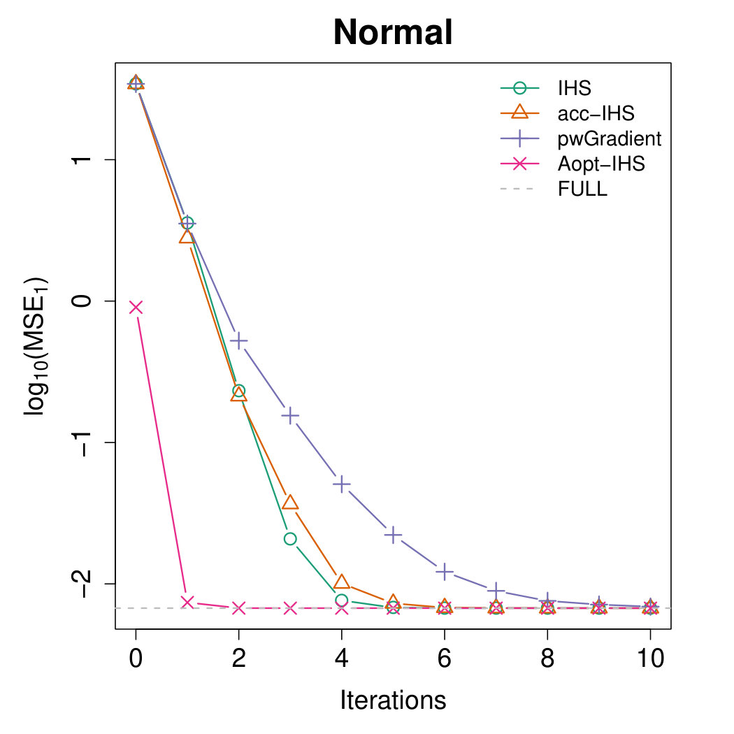 Figure 1
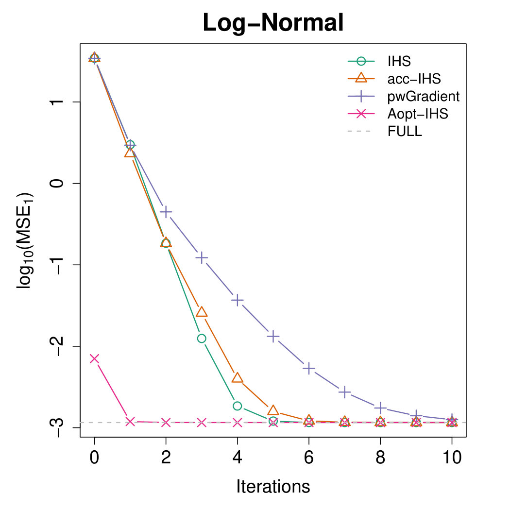 Figure 2
 Figure 3
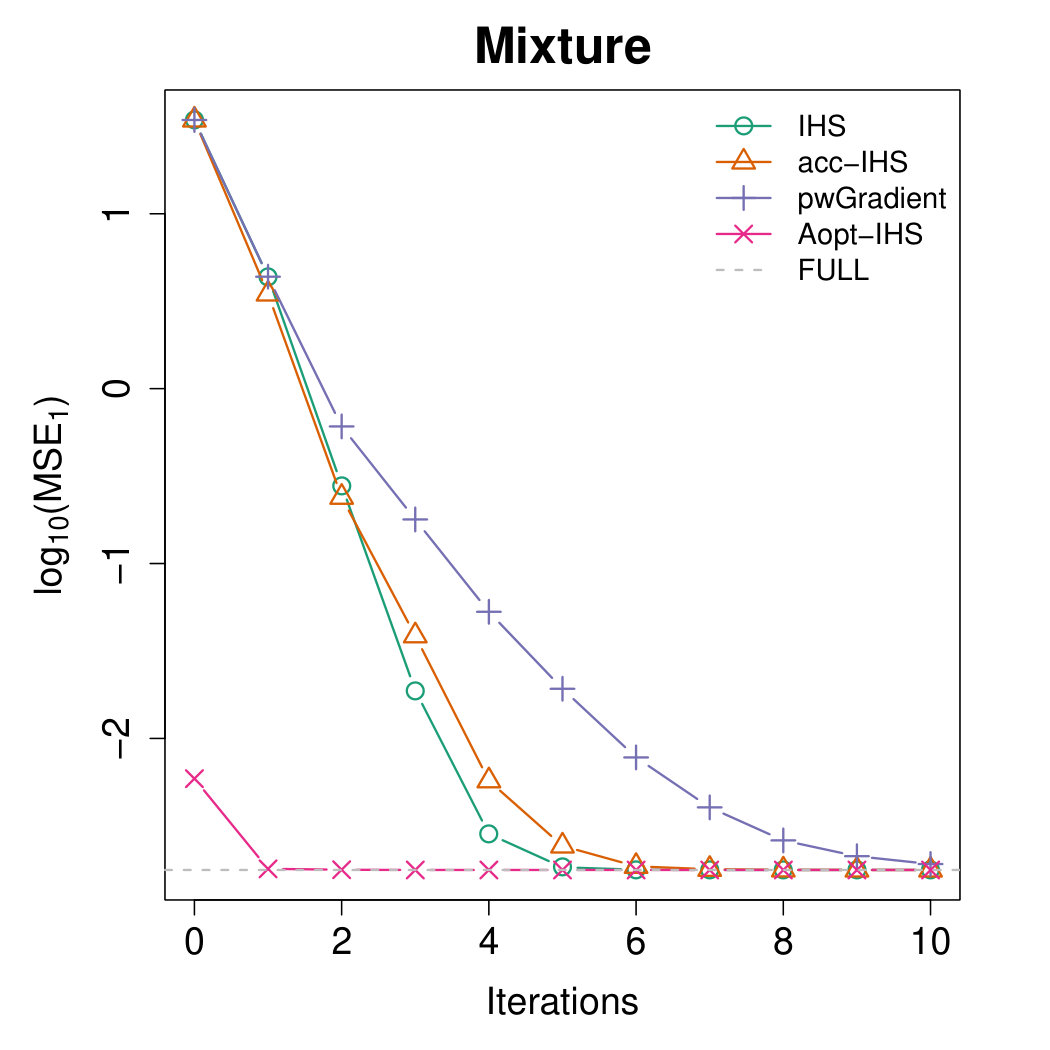 Figure 4
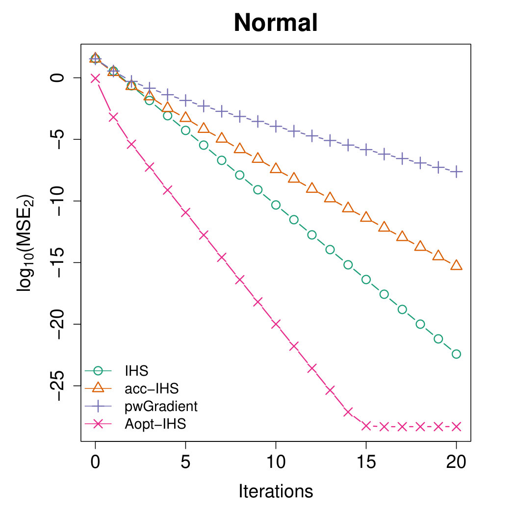 Figure 5
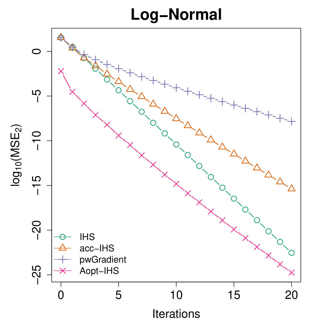 Figure 6
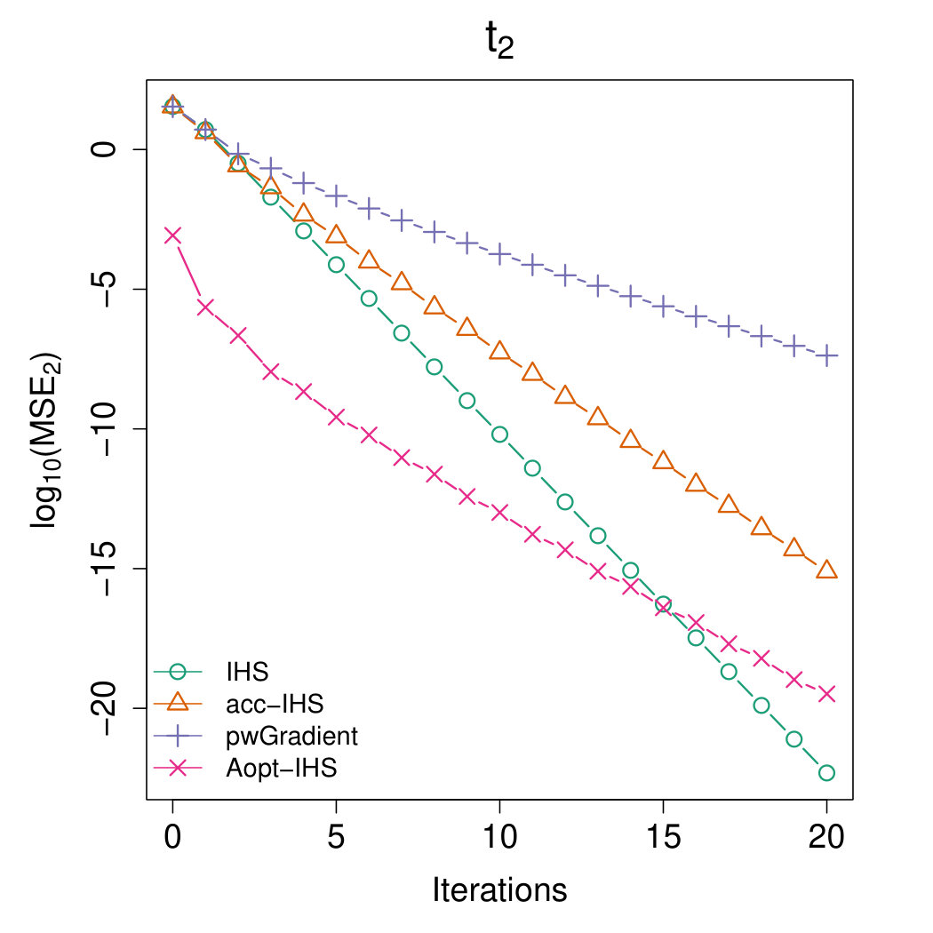 Figure 7
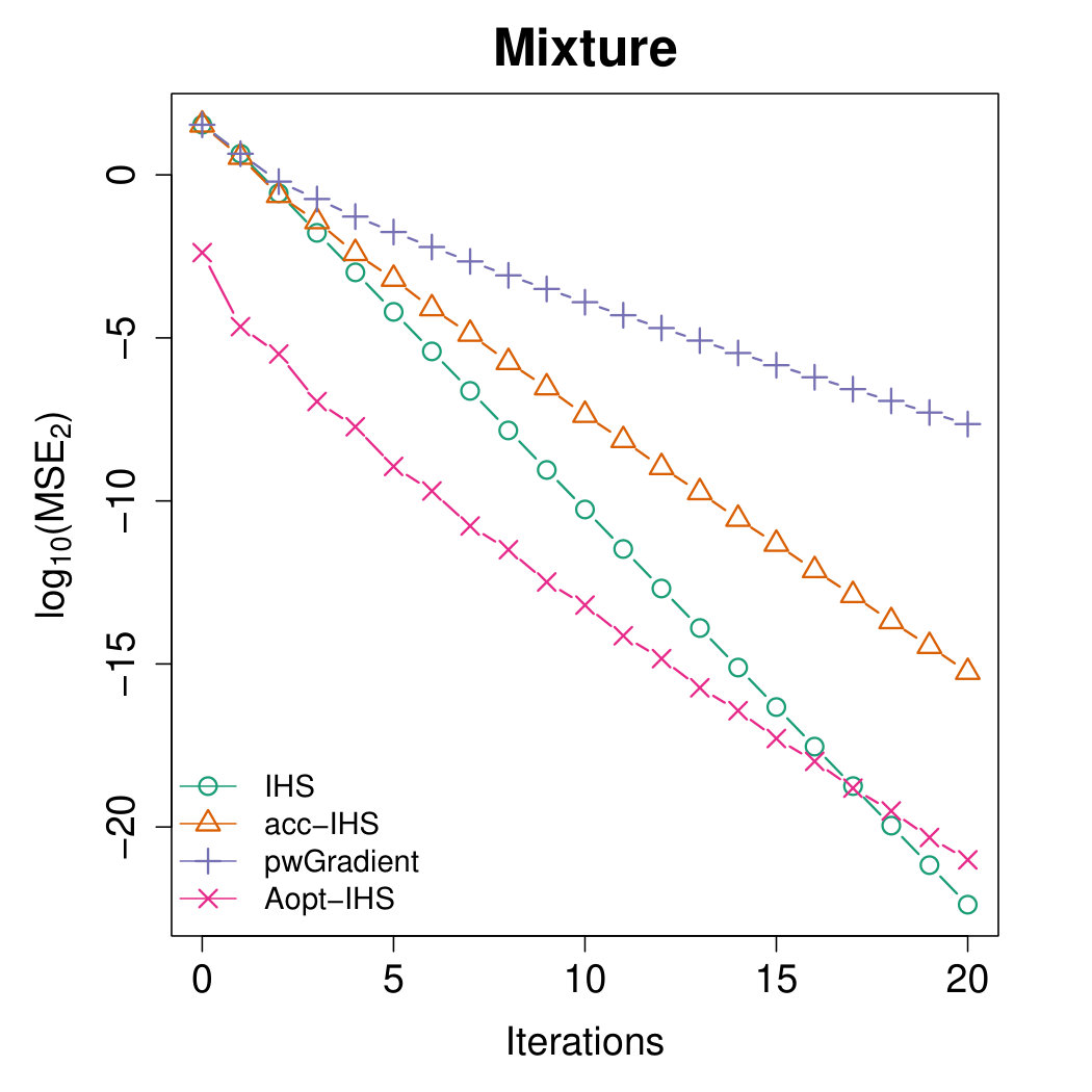 Figure 8
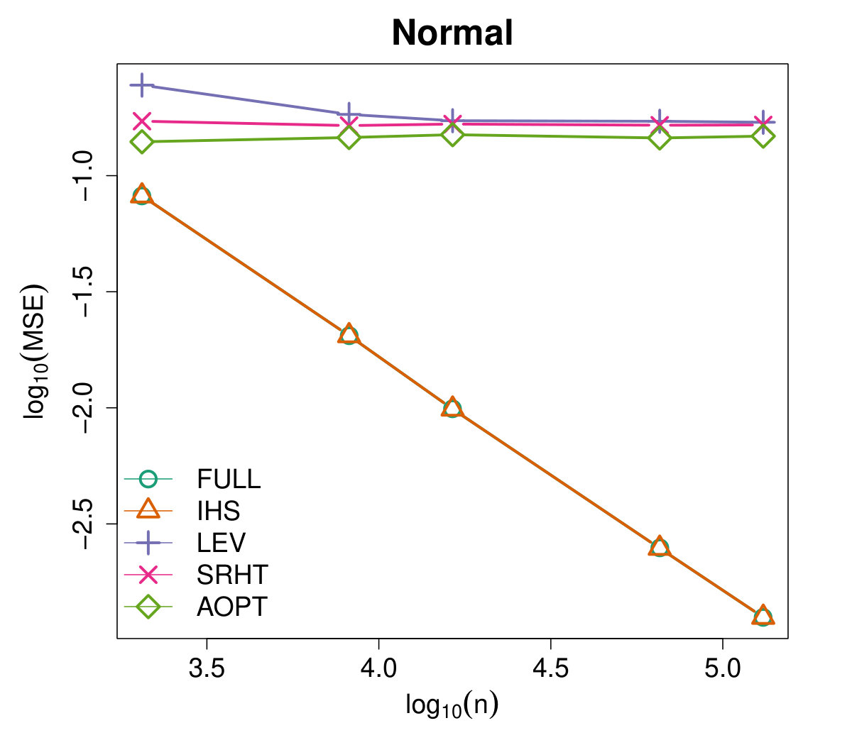 Figure 9
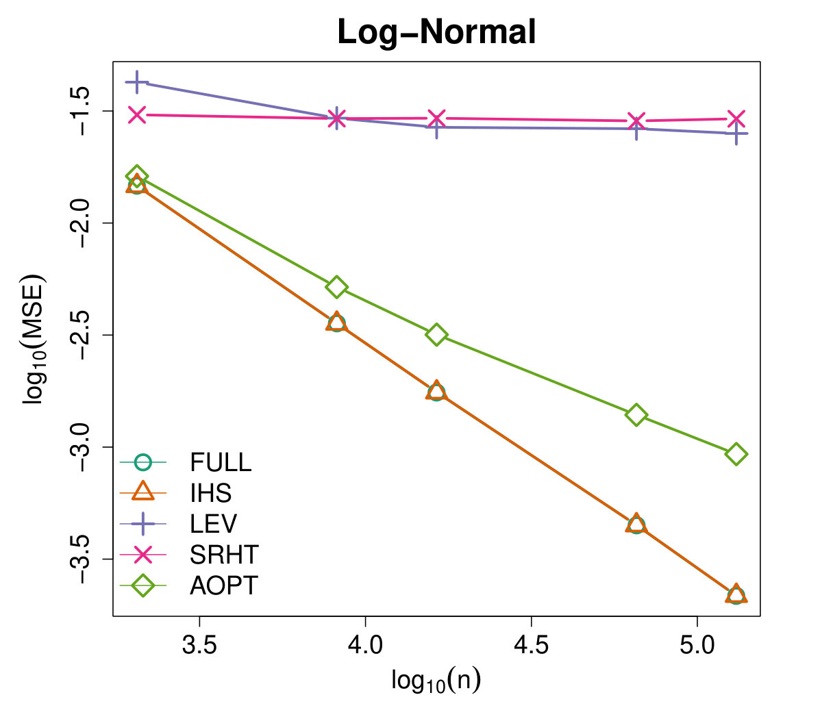 Figure 10
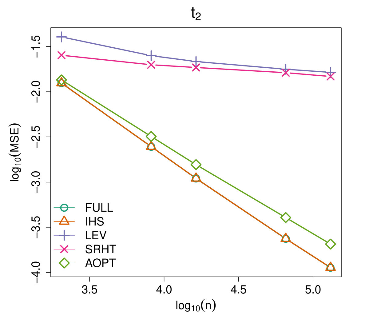 Figure 11
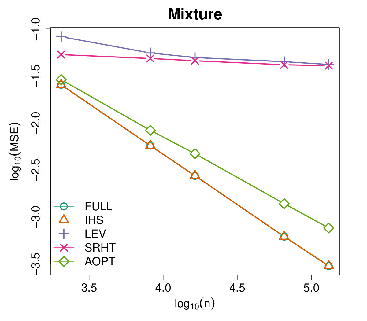 Figure 12
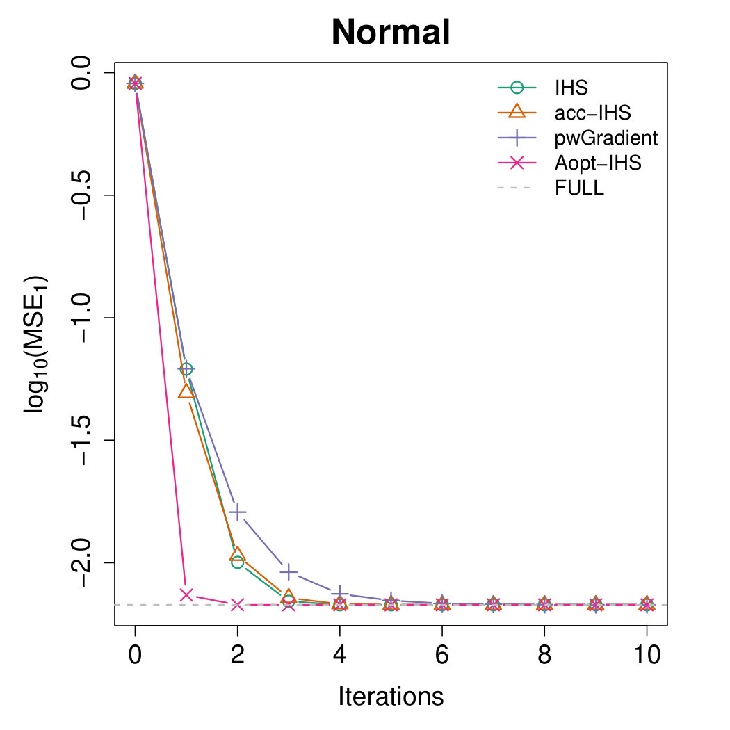 Figure 13
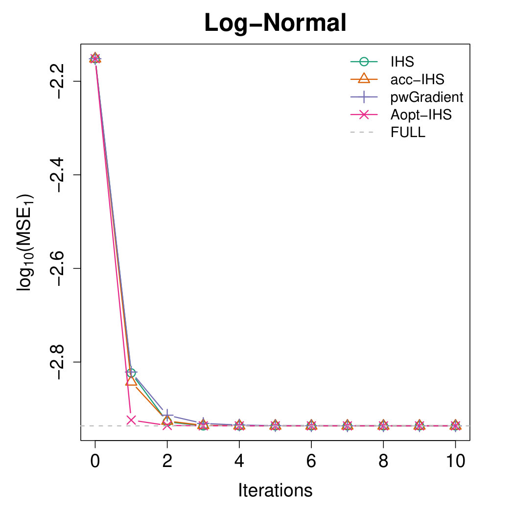 Figure 14
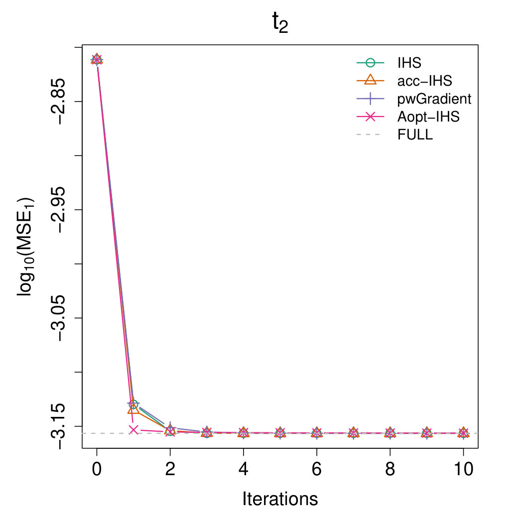 Figure 15
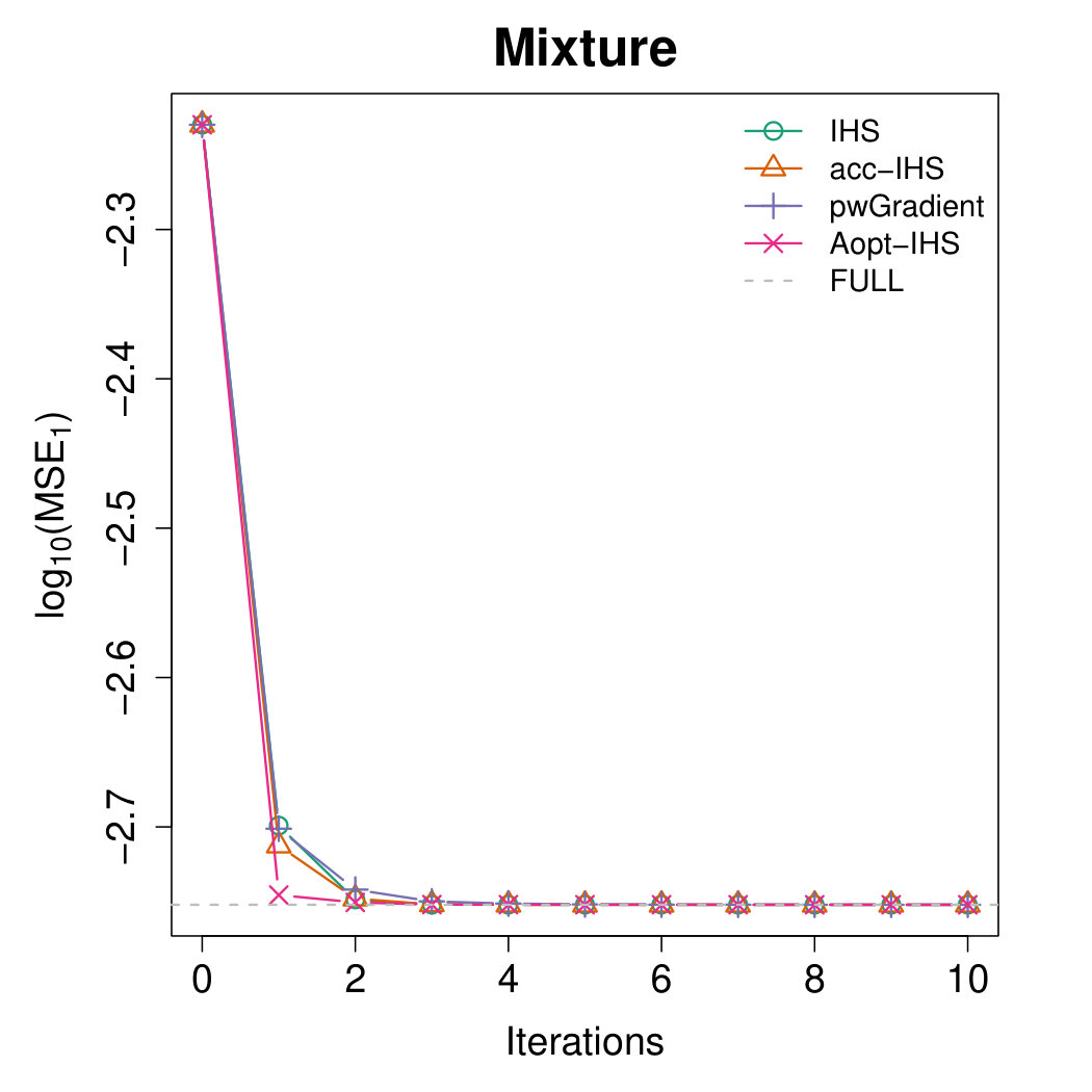 Figure 16
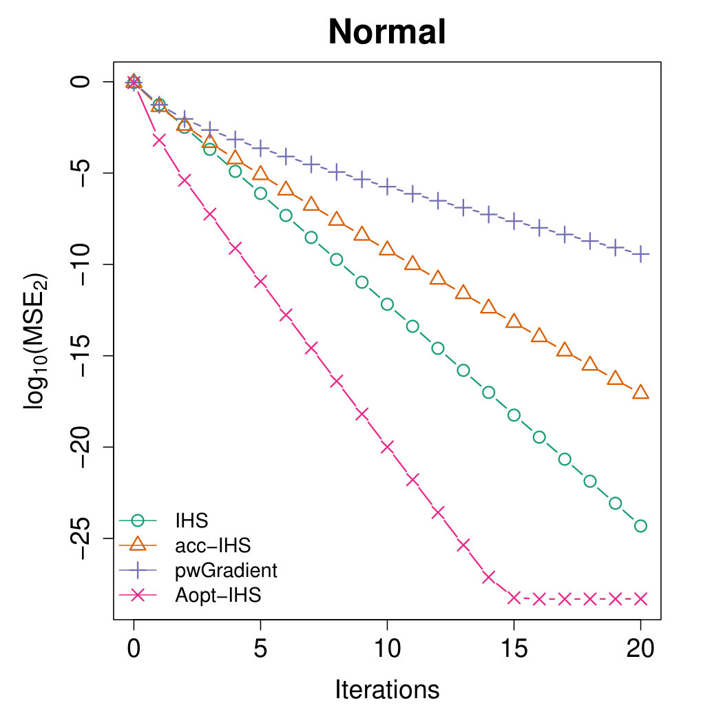 Figure 17
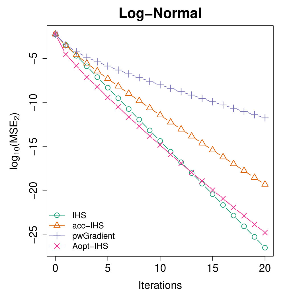 Figure 18
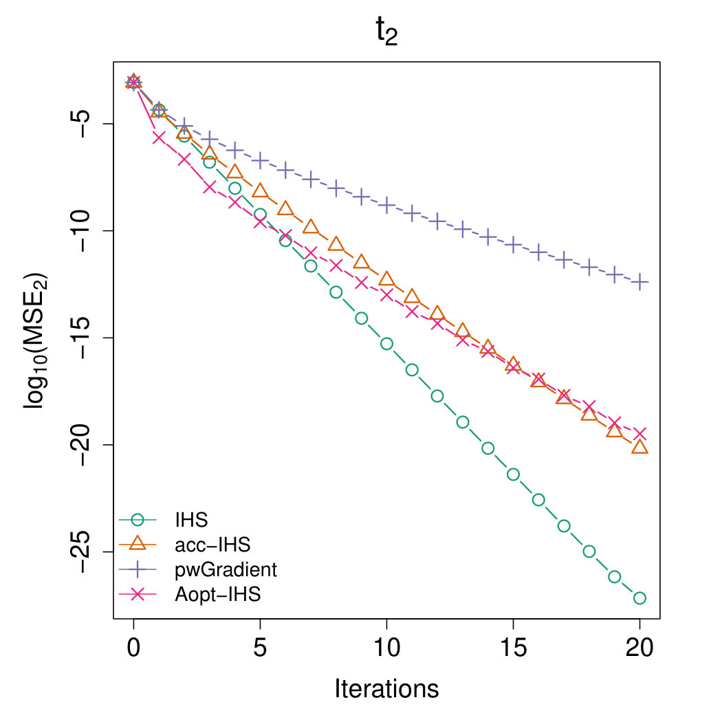 Figure 19
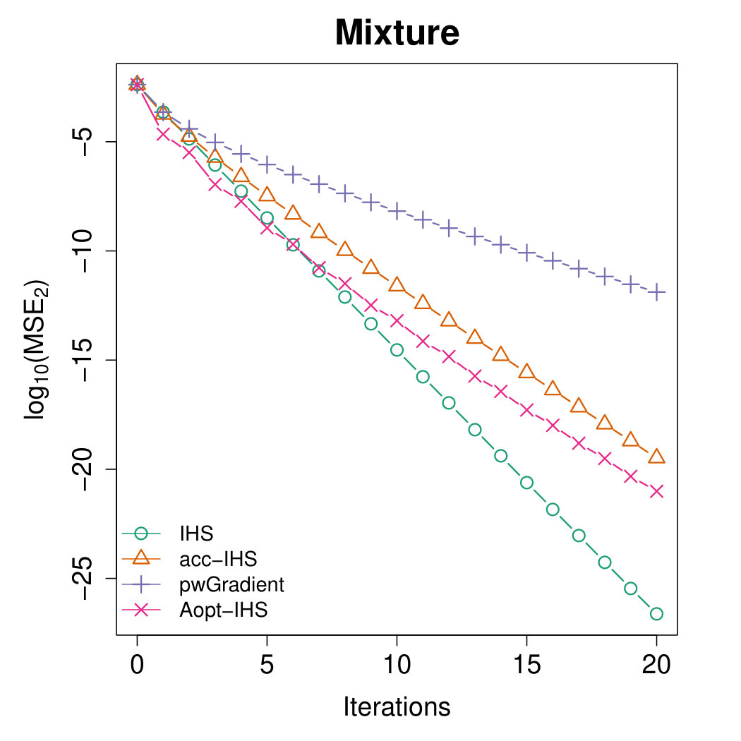 Figure 20
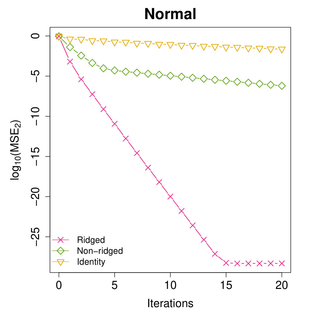 Figure 21
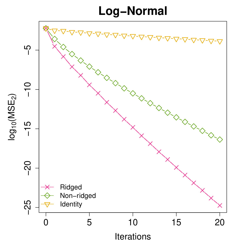 Figure 22
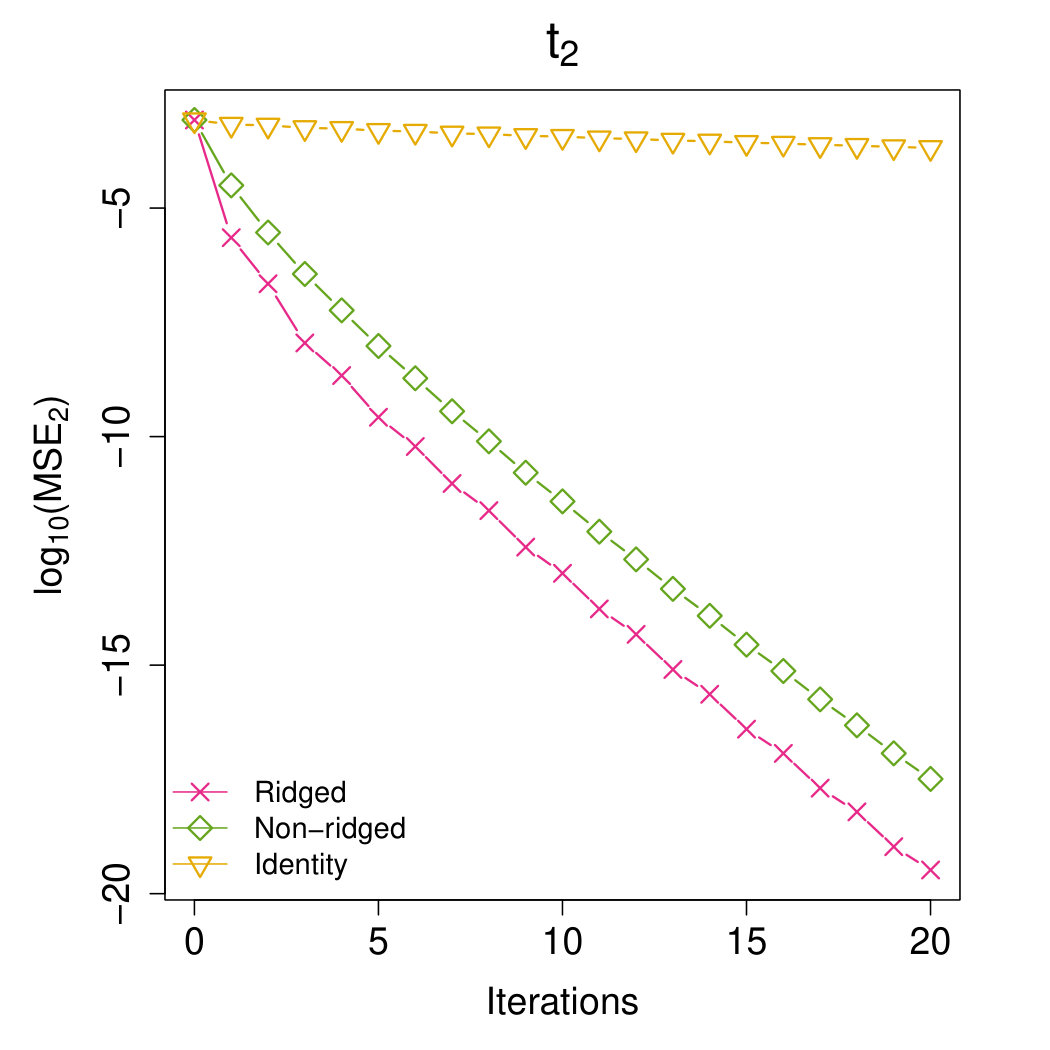 Figure 23
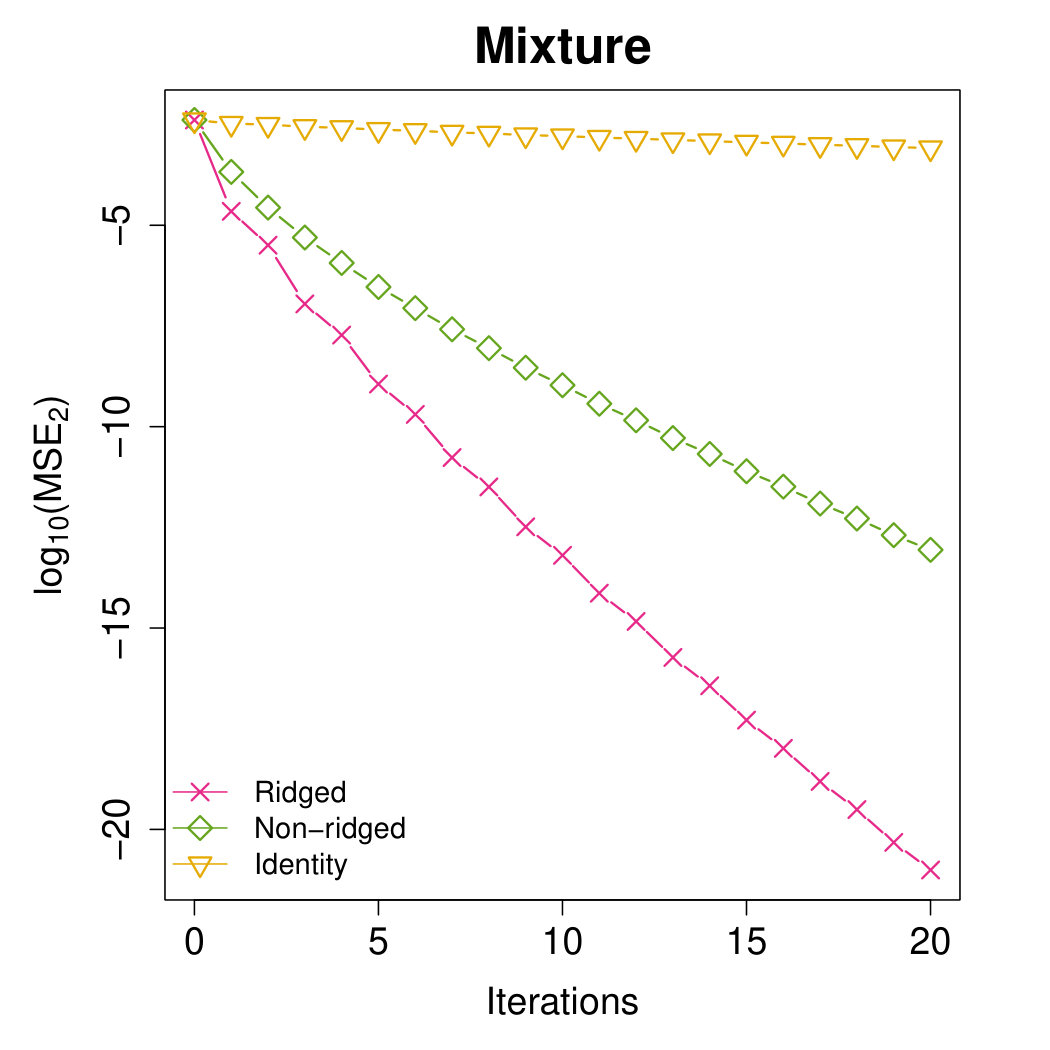 Figure 24
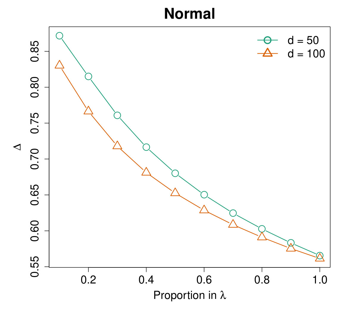 Figure 25
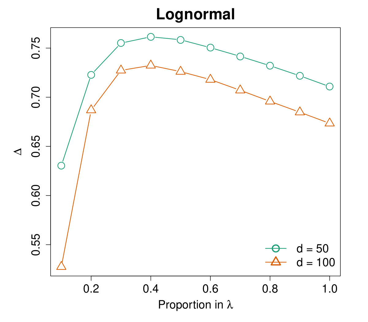 Figure 26
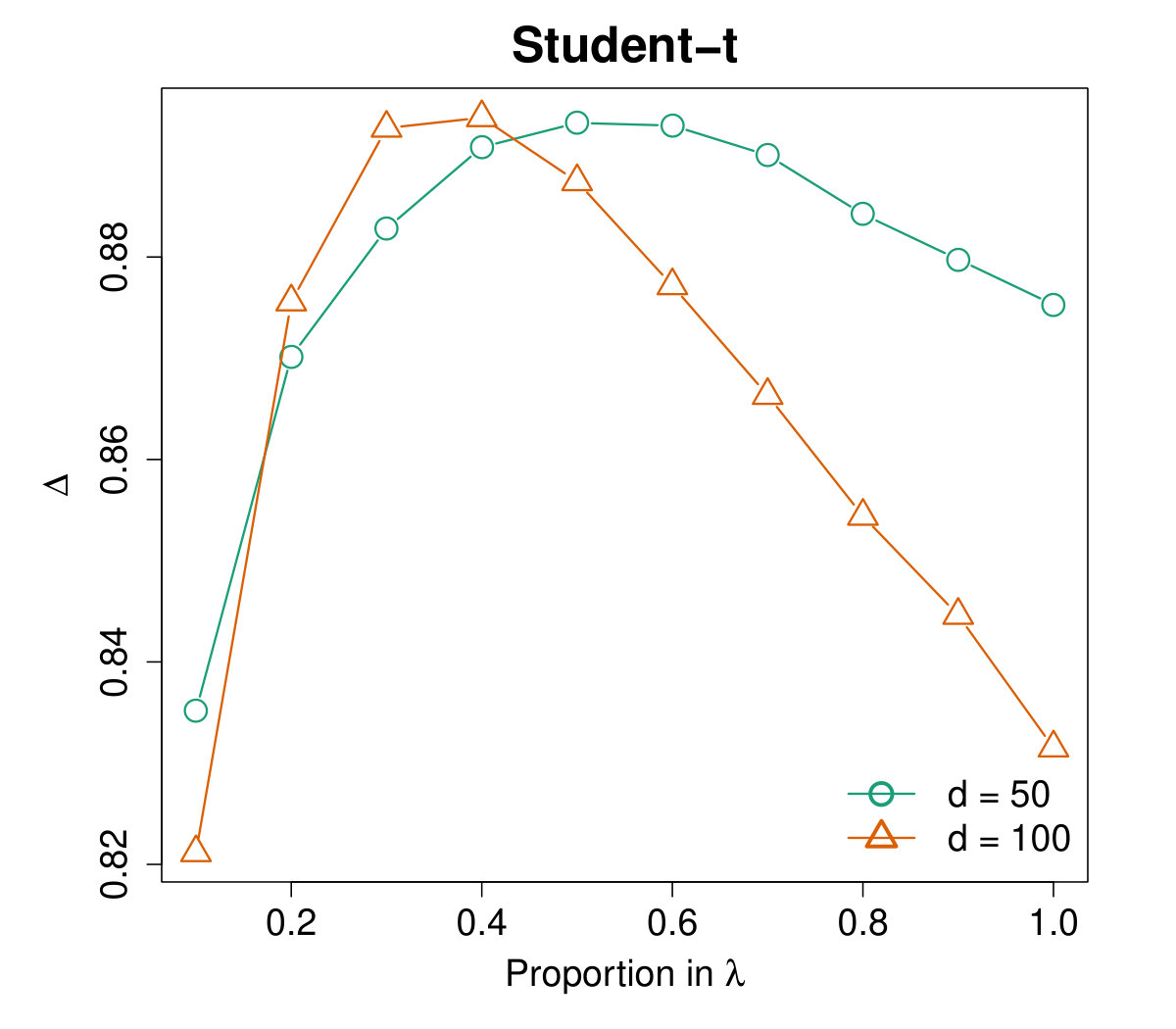 Figure 27
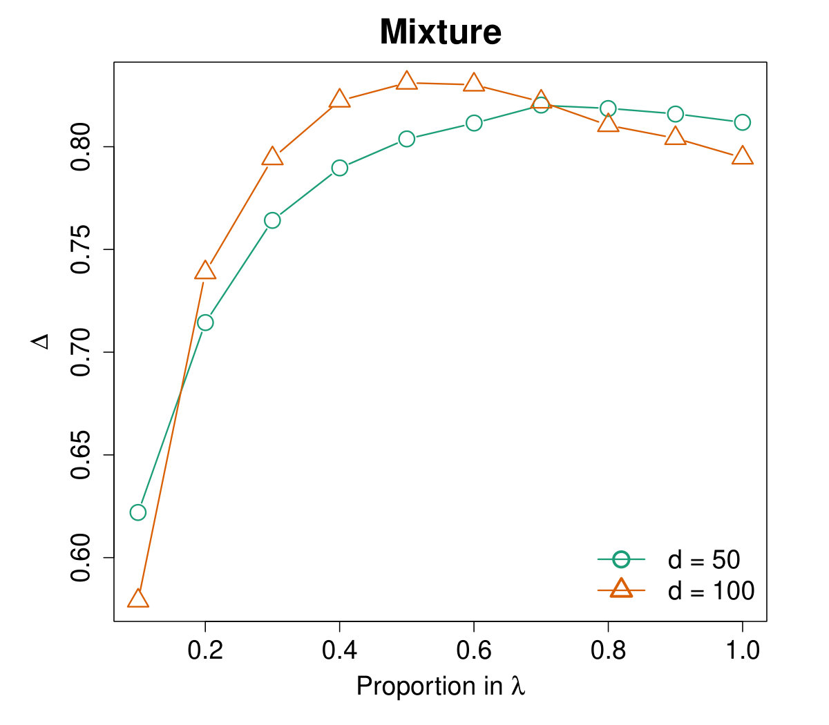 Figure 28
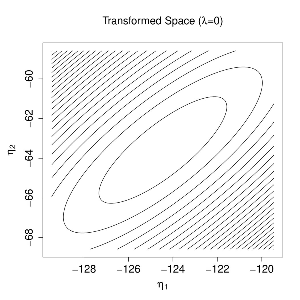 Figure 29
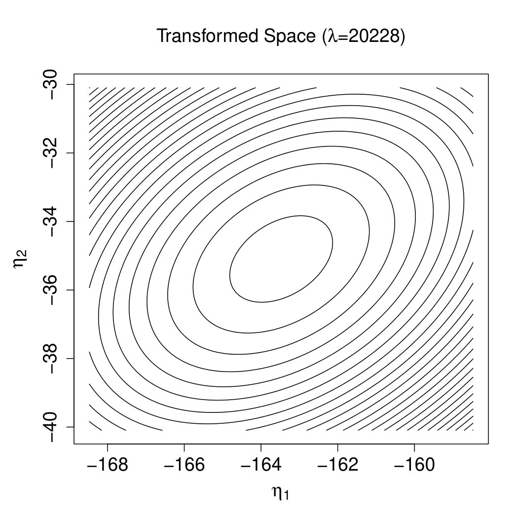 Figure 30
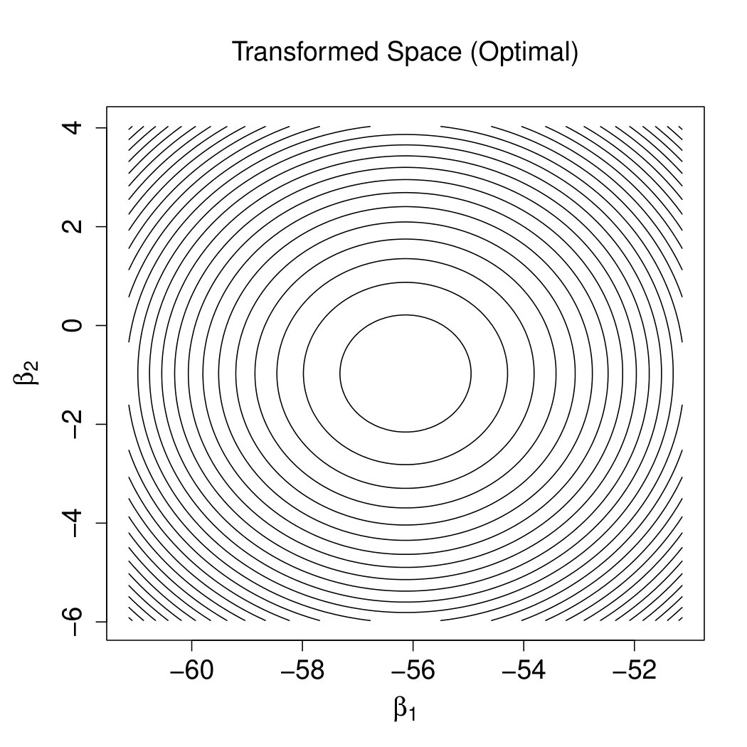 Figure 31
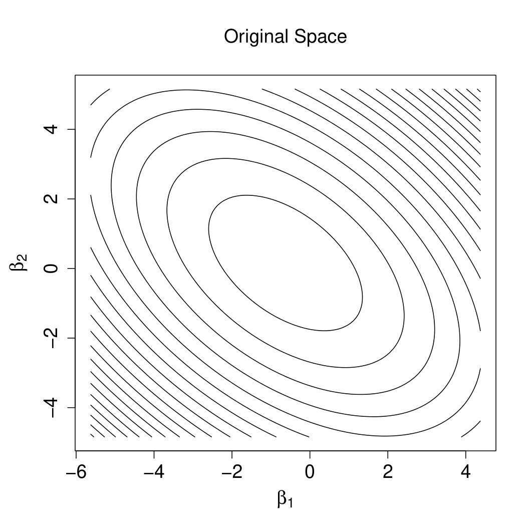 Figure 32
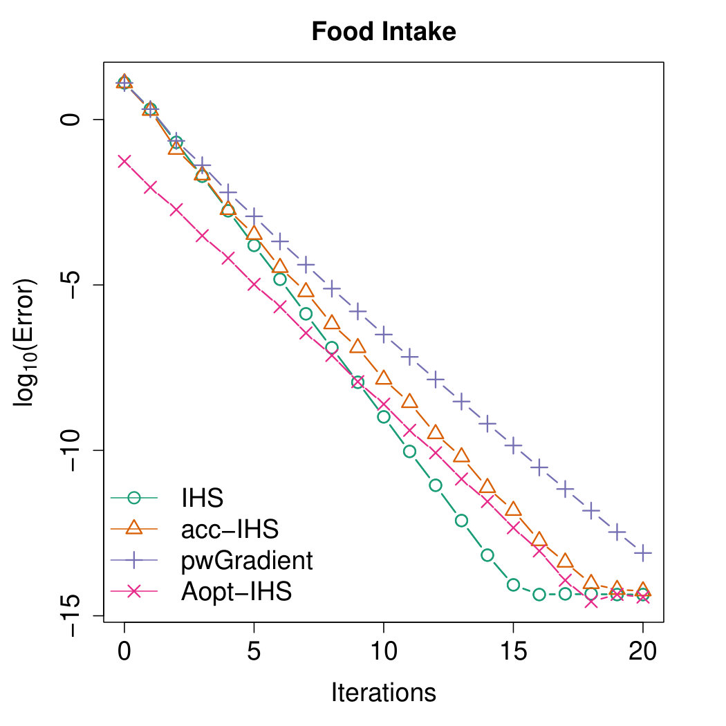 Figure 33
| Normal | Log-Normal | Mixture | ||
| -4.56 | 0.39 | 0.76 | 0.42 | |
| 0.87 | 0.76 | 0.89 | 0.79 | |
| SRHT | 0.55 | 0.52 | 0.75 | 0.70 |
| -7.62 | -0.41 | 0.63 | -0.01 | |
| 0.83 | 0.73 | 0.90 | 0.82 | |
| SRHT | -0.04 | 0.05 | 0.46 | 0.32 |
| Method | Normal | Log-Normal | Mixture | |||||
|---|---|---|---|---|---|---|---|---|
| Time(s) | Iter | Time(s) | Iter | Time(s) | Iter | Time(s) | Iter | |
| IHS | 15.28 | 18.30 | 14.83 | 18.25 | 15.63 | 18.43 | 15.21 | 18.38 |
| acc-IHS | 5.63 | 25.95 | 5.20 | 25.87 | 5.57 | 26.17 | 5.88 | 26.05 |
| pwGradient | 8.54 | 46.99 | 8.19 | 47.40 | 8.98 | 47.34 | 9.22 | 47.67 |
| Aopt-IHS | 3.01 | 10.27 | 3.90 | 14.97 | 3.75 | 12.65 | 4.74 | 17.39 |
| IHS | 53.55 | 27.29 | 54.89 | 27.16 | 48.17 | 27.51 | 43.31 | 27.40 |
| acc-IHS | 19.59 | 40.64 | 19.59 | 40.51 | 17.11 | 41.01 | 15.42 | 40.92 |
| pwGradient | — | diverge | — | diverge | — | diverge | — | diverge |
| Aopt-IHS | 11.28 | 19.44 | 11.16 | 19.07 | 11.32 | 22.78 | 9.48 | 20.45 |
Peer Reviews
No public reviews on file for this paper yet. If you reviewed it on a platform where reviews are public (OpenReview, ICLR, NeurIPS, ICML), you can paste yours below so the community can read it here.
Videos
No videos yet. Explain this paper in a talk, walkthrough, or lecture? Add one.
Taxonomy
TopicsIndoor and Outdoor Localization Technologies · Sparse and Compressive Sensing Techniques · Robotics and Sensor-Based Localization
Adaptive Iterative Hessian Sketch via -Optimal Subsampling
Aijun Zhang∗, Hengtao Zhang and Guosheng Yin
Department of Statistics and Actuarial Science, The University of Hong Kong
Pokfulam Road, Hong Kong
Abstract
Iterative Hessian sketch (IHS) is an effective sketching method for modeling large-scale data. It was originally proposed by Pilanci and Wainwright (2016; JMLR) based on randomized sketching matrices. However, it is computationally intensive due to the iterative sketch process. In this paper, we analyze the IHS algorithm under the unconstrained least squares problem setting, then propose a deterministic approach for improving IHS via -optimal subsampling. Our contributions are three-fold: (1) a good initial estimator based on the -optimal design is suggested; (2) a novel ridged preconditioner is developed for repeated sketching; and (3) an exact line search method is proposed for determining the optimal step length adaptively. Extensive experimental results demonstrate that our proposed -optimal IHS algorithm outperforms the existing accelerated IHS methods. Keywords: Hessian sketch, Subsampling, Optimal design, Preconditioner, Exact line search, First-order method.
1 Introduction
Consider the linear model with the response vector , the design matrix and the noise term satisfying and . The unknown parameter can be efficiently estimated by the method of least squares:
[TABLE]
which is of computational complexity . For the massive data with , the least squares method would become computationally expensive, and it may exceed the computing capacity.
Faster least squares approximation can be achieved by the randomized sketch proposed by Drineas et al., (2011). It relies on a proper random matrix with . The ways to generate random matrix are divided into three main categories: subsampling, random projection and their hybrid. A widely known subsampling method is based on statistical leverage (LEV) scores (Drineas et al.,, 2006; Mahoney et al.,, 2011; Drineas et al.,, 2012; Ma et al.,, 2015). The random projection approach includes the subsampled randomized Hadamard transformation (SRHT) (Drineas et al.,, 2011; Boutsidis and Gittens,, 2013) and the Clarkson–Woodruff sketch (Clarkson and Woodruff,, 2013). The hybrid approach is to combine subsampling and random projection, see e.g. McWilliams et al., (2014).
When a sketching matrix is fixed, there exist different sketching schemes, including the classical sketch (CS), the Hessian sketch (HS) and the iterative Hessian sketch (IHS). The widely adopted CS uses the sketched data pair for approximating by
[TABLE]
Pilanci and Wainwright, (2016) showed that is suboptimal in the sense that it has a substantially larger error than with respect to the ground truth . They introduced the HS estimator based on the partially sketched data ,
[TABLE]
and furthermore the IHS estimator based on iterative sketched data ,
[TABLE]
where , with the initial being provided. Unlike the CS and HS estimators, the IHS estimator is guaranteed to converge to upon some good event conditions (Pilanci and Wainwright,, 2016).
The IHS can be interpreted as a first-order gradient descent method with a series of random preconditioners subject to the unit step length. The preconditioner is widely used to boost optimization algorithms (Knyazev and Lashuk,, 2007; Gonen et al.,, 2016). However, the IHS is computationally intensive since in every iteration has to be evaluated for a new random sketching matrix . To speed up the IHS, Wang and Xu, (2018) proposed the pwGradient method to improve the IHS by a fixed well-designed sketching matrix, in which case the IHS reduces to a first order method with a constant preconditioner. Meanwhile, Wang et al., (2017) proposed another accelerated version of IHS with the fixed sketching matrix, while adopting conjugate gradient descent. Note that all these sketch methods are based on randomized sketching matrices.
In this paper we propose to reformulate the IHS estimator by a linear combination of the initial and the full data estimator . Such reformulation enables us to find a sufficient isometric condition on the sketching matrices so that is guaranteed to converge to with geometric convergence. It then motivates us to propose a deterministic approach for improving the IHS based on -optimal subsampling and adaptive step lengths, which modifies the original second-order IHS method to be an adaptive first-order method. In summary, we improve the IHS method with the following three contributions:
- •
Good initialization. A good initialization scheme can reduce the inner iteration rounds of IHS while still delivering the same precision. We suggest to initialize the IHS with the classical sketch based on the -optimal deterministic subsampling matrix. To our best knowledge, this is the first attempt to take initialization into account for improving the IHS method.
- •
Improved preconditioner. It is critical to find a well-designed preconditioner so that it may be fixed during the iterative sketch process. We propose to construct the preconditioner from -optimal subsample and refine it by adding a ridge term. Unlike complicated random projection-based methods, we obtain our preconditioner at a low cost by recycling the subsamples in initialization and make no assumption on the sample size.
- •
Adaptive step lengths. We modify the IHS to be an adaptive first-order method by using a fixed preconditioner subject to variable step lengths. The step lengths at each iteration are determined by the exact line search, which ensures the algorithm to enjoy the guaranteed convergence.
Through extensive experiments, our proposed method is shown to achieve the state-of-art performance in terms of both precision and speed when approximating both the ground truth and the full data estimator .
2 Reformulation of IHS
The original IHS algorithm is displayed in Algorithm 1. For simplicity, we omit the superscript from . As for the sketch matrix, we use SRHT as it is widely adopted in the literature. Following Tropp, (2011) and Lu et al., (2013), when where is a positive integer, the SRHT sketch matrix is given by
[TABLE]
where is an matrix with rows chosen uniformly without replacement from the standard bases of , is a normalized Walsh–Hadamard matrix of size , and is an diagonal matrix with i.i.d. Rademacher entries. Note that when is not the power of two, is padded with zeros until achieves the next greater power of two.
In what follows, we present a novel reformulation of IHS. At each step, the update formula in Algorithm 1 can be rewritten as
[TABLE]
By (4), we can derive the following lemma by mathematical induction.
Lemma 1
Given an initializer and a series of independent sketch matrices , for any positive integer , we have
[TABLE]
where and .
Lemma 1 reveals that is a linear combination of the initial and the full data estimator , with the re-weighting matrices during the iterations. We can therefore study the convergence properties of by looking into or . The following theorem provides a sufficient isometric condition for the convergence guarantee.
Theorem 1
Given an initial estimator and a set of sketch matrices , the IHS estimator converges to with geometric convergence,
[TABLE]
provided that for any and and for any \bm{a}\in\mathbb{R}^{d}$$\backslash\{\bm{0}\},
[TABLE]
Proof 1
From Lemma 1, we have
[TABLE]
Thus, it holds that
[TABLE]
Note that
[TABLE]
where . Since shares the same eigenvalues with (See 6.54 in Seber, (2008)), we have
[TABLE]
[TABLE]
From the conditions (7), we know that
[TABLE]
for any \bm{b}=\bm{Q}^{1/2}\bm{a}\in\mathbb{R}^{d}$$\backslash\{\bm{0}\}. Thus, we have that
[TABLE]
So, (8) becomes
[TABLE]
It is clear that the rate , so converges to .
Theorem 1 is meaningful in different ways. Firstly, when and , it can be checked that Theorem 1 corresponds to the main result of Pilanci and Wainwright, (2016) under the so-called good event condition. It also mimics the Johnson-Lindenstrauss lemma (Johnson and Lindenstrauss,, 1984) when . Moreover, our theorem makes no assumption about the randomness of and it is applicable to all kinds of sketch matrices satisfying (7). In the case of random , let , be the orthonormal basis of ’s column space. It suffices to obtain (9) and hence (7) once satisfies . Theorem 2.4 in Woodruff et al., (2014) showed one way to construct such random with high probability.
The original IHS method requires calculating with time complexity repeatedly for each ; see Section 2.5 of Pilanci and Wainwright, (2016). Theorem 1 indicates that a fixed sketch matrix such can also ensure the convergence if the condition (7) is satisfied. This result provides enables us to reduce the computational cost for the original IHS method. For example, Wang and Xu, (2018) proposed the pwGradient method to improve the IHS by constructing a well-designed sketch algorithm, which can be viewed as an application of Theorem 1 by letting , and .
In the meanwhile, we can also interpret the IHS approach based on a transformed space. Let the preconditioner , multiply to the both sides of (2), and denote and for . Then, we have
[TABLE]
which corresponds to the gradient descent update when minimizing the following least squares objective
[TABLE]
The one-to-one mapping between and ensures that one can show the convergence of and obtain its optima via equivalently analyzing . Based on this observation, Wang et al., (2017) proposed the acc-IHS method by fixing the preconditioner and replacing the gradient descent with the conjugate counterpart in the transformed parameter space. It is worth mentioning that both the pwGradient and acc-IHS methods belong to the randomized approach based on random projections, while the SRHT sketching needs to operate on all the entries of . We hence seek to improve the IHS method in a more efficient and deterministic way.
3 Adaptive IHS with -Optimal Subsampling
We extend the concept of sketch matrix from randomized settings to deterministic settings, by introducing to indicate where an observation is selected, i.e., if sample or is included, otherwise. It is assumed that , which implies that the corresponding sketch matrix satisfies . It is our objective to find a good subject to certain optimality criterion.
3.1 -Optimal Classical Sketch
The convergence of also depends on as shown in (6), which motivates us to find a good initializer. We achieve this goal by proposing an -optimal estimator under the classical sketch scheme. Suppose that we select a subset of observations. The least squares estimator based on the subdata and the corresponding covariance matrix are given by
[TABLE]
Let . Following the -optimality criterion in experimental design (Pukelsheim,, 1993), we seek the subdata as indicated by that minimizes the averaged variance of , which is proportional to the trace of . Formally, our goal can be formulated as the following discrete optimization problem,
[TABLE]
However, it is NP-hard to solve it exactly, so we turn to derive a upper bound of , which leads to Algorithm 2.
Theorem 2
Let , denote the condition number, be the collection of all feasible solutions and correspond to the smallest eigenvalue. Assuming that , for any given ,
[TABLE]
Proof 2
Let , , be the largest eigenvalue, denote the SVD of where , and . Therefore, we have
[TABLE]
It is easy to check that where the first inequality follows and 10.47 in Seber, (2008). We can further conclude as . According to the extension of Corollary 5.6.16. in Horn and Johnson, (2012), we have
[TABLE]
So the trace in (13) can be further bounded as follows,
[TABLE]
Note that the denominator
[TABLE]
where the second and third equations follow the definition of eigenvalue and ’s SVD respectively. With 6.76 in Seber, (2008), the denominator is lower bounded by
[TABLE]
Similarly, for the nominator, we have
[TABLE]
The inequality follows by plugging above two bounds into (14).
By Theorem 2, we can seek an approximately -optimal design by shrinking its upper bound, i.e., maximizing . Our subsampling approach is described as follows.
Remark 1
The time for norm calculation is , while sorting requires on average operations (Martınez,, 2004). For step 3, it costs to obtain . In total, the time complexity of Algorithm 2 is . The time can be further reduced to when it comes to , which is a common scenario for massive data. Furthermore, this constraint can also be a reference for the sketch size determination as it implies that should not exceed for an efficient complexity. From the time complexity perspective, our algorithm is as efficient as the -optimality based method in Wang et al., (2018), while ours is more suitable for parallel computation.
Remark 2
In practice, when the data matrix is centered and scaled initially, our algorithm tends to choose the extreme samples with the farthest distances to the center, which is consistent with the conclusion in Wang et al., (2018).
As shown in Figure 1, the performance of the -optimal method uniformly dominates that of randomized sketch matrices and classical sketching scheme. Furthermore, the MSE of our approach decreases with an increase of . In this regard, our -optimal estimator serves as a good initialization for further enhancements.
3.2 Improved Preconditioner
Note that is mainly determined by a set of matrices . Rather than specifying ’s by repeatedly sketching in IHS or fixing in pwGradient and acc-IHS, we make a compromise by defining , that is,
[TABLE]
where . We consider the -optimal Hessian sketch in order to specify a deterministic preconditioner . Similarly, we can obtain the estimator of Hessian sketch and its covariance matrix based on an optimality criterion,
[TABLE]
where . The next theorem provides a upper bound for the trace of the covariance matrix.
Theorem 3
Under the same conditions of Theorem 2, for any , we have
[TABLE]
Proof 3
Note that
[TABLE]
Therefore the above inequality can be easily obtained by applying Theorem 2.
Theorem 3 shows that the -optimal design of Hessian sketched estimator can also be approximated via finding the samples with largest norm. The samples selected for initialization can be recycled for constructing the preconditioner. We find that adding a ridge term can further improve our preconditioner
[TABLE]
The rationale is demonstrated by Figure 2. Note that the effectiveness of the precondtioner is measured by (Benzi,, 2002), which should be close to 1. And can be visualized by the contour plot of in the two-dimensional cases. Specifically, the flat degree of the contour plot indicates the size of the condition number. The larger the condition number, the more circular the contour plot. The optimal transformation is as shown by Figure 2(b). Observing Figures 2(a) and 2(c), is still close to the , i.e., the preconditioner fails. After ridging, our preconditioner shrinks the major radius in Figure 2(c) and render the transformation to reach optimality as shown by Figure 2(d).
3.3 Exact Line Search
Using the improved preconditioner of the form (16), the adaptive first-order IHS estimator (15) can be rewritten as
[TABLE]
for . To determine adaptively, we note that it actually corresponds to the learning rate of the first order method in the transformed space. Recall that the learning rate in (10) is fixed as unit 1, which may be suboptimal and does not lead to the largest descent for every iteration. We hence fulfill the potential of IHS by exact line search. Specifically, let
[TABLE]
be the update direction at the th iteration, the optimal step lengths are determined by adaptively minimizing the univariate function . It is easy to show that
[TABLE]
where . Moreover, with the above , the first-order method becomes steepest descent in the transformed space with the guaranteed convergence; see Theorem 3.3 in Nocedal and Wright, (2006). Thus it also converges in the original space by the one-to-one mapping between and .
In summary, we present the adaptive -optimal IHS in Algorithm 3. The algorithm uses a pre-specified loop number , and it can be modified by early stopping strategy, e.g. when the difference between and is below a tolerance threshold.
4 Numerical Experiments
4.1 Simulated Data Analysis
Data Generation.
We generate data by following the experimental setups of Wang et al., (2018). All data are generated from the linear model with the true parameter being i.i.d variates and . Let be the covariance matrix where its entry is for , and is the indicator function. We consider four multivariate distributions for covariates .
- (1)
A multivariate normal distribution . 2. (2)
A multivariate log-normal distribution which is generated by taking the exponential transformation of . 3. (3)
A multivariate distribution with degrees of freedom . 4. (4)
A mixture distribution composed of five different distributions , , , , \mbox{\rm LN}({\color[rgb]{0,0,0}{}\bm{0}},\bm{\Sigma}) with equal proportions, where represents elements from independent uniform distributions.
To remove the effect of the intercept, we center the data. Unless particularly stated, we set and present the results averaged over replications.
Choice of Preconditioner.
To assess the quality of the preconditioner that is a positive definite matrix, we first define the measure as the ratio of improvement with respect to the condition number,
[TABLE]
For a good preconditioner, its measure should be positive and close to 1. In contrast, a preconditioner with negative value would worsen the condition number .
To choose the ridge parameter , we calculate the averaged values on different distributions versus as a proportion of . Specifically, let and the proportion take values from to with step size . The results are plotted in Figure 3, which shows that the curves are similar on heavy-tailed distributions but not so consistent for the normal case. Through extensive experiments, as a rule of thumb, we suggest that takes value for relatively concentrated data and for heavy-tailed distributions.
Table 1 presents the averaged values of the proposed preconditioner (16) for different distributions with dimensionality and , respectively. We use to denote for the normal distribution and for other cases. The results are compared with and the SRHT scheme. It is clear that the preconditioner with parameter uniformly dominates in all cases. Such superiority is especially significant for the cases with , i.e., when is relatively large. Furthermore, note that when , and . Therefore the ridged combination indeed brings significant improvement on the preconditioner.
Comparative Study.
We compare the proposed deterministic -optimal IHS to the original randomized IHS Pilanci and Wainwright, (2016), as well as two other improved IHS methods: acc-IHS Wang et al., (2017) and pwGradient Wang and Xu, (2018). The initial estimators of these benchmark methods are set to be the vector zero as suggested in the original papers. Two empirical MSE criteria are used to evaluate the algorithm:
[TABLE]
where denotes the estimator of the th iteration in the th round, and the trimmed mean with fraction 0.025 is applied to handle the effects of abnormal situations. We record MSEs from the [math]th iteration (i.e. initialization stage) and set the sketch dimension to be at every iteration. Note that the randomized IHS requires independent sketch matrix for each iteration, while the other methods reuse the same sketch matrix for each iteration.
Figures 4 and 5 illustrate the advantages of our proposed Aopt-IHS method. Firstly, the superiority of initialization can be thoroughly reflected by the flat curve in Figure 4, as well as the lower starting values in Figure 5. During the iterations, the outperformance of the proposed method can be reflected in Figure 5. Specifically, given the convergent property of , the curve slope reflects the convergence rate while the intercept or the starting point measures the effect of the initialization. From the plots, the proposed Aopt-IHS method not only outperforms in the initialization but also demonstrates a decent convergence rate that is competitive to pwGradient and it is even sharper than IHS for the normal case.
To compare the computational time, we present in Table 2 the averaged run time for each method for achieving the precision in , as well as the required numbers of iterations. Note that the time for computing in the update formula is not counted for all methods. Table 2 shows that our method can attain the same precision with fewer iterations and shorter time.
4.2 Real Data Analysis
Finally, we apply the proposed method to a real food intake dataset111Data can be found in https://www.icpsr.umich.edu/icpsrweb/ICPSR/studies/21960#.. This data, consisting of three sub-files, records the information on one-day dietary intakes of male residents in the United States with age from 19 to 50 in 1985. We consider the largest food intake file that includes how much and when the food items are taken. This sub-file has samples and we are interested in the linear regression model between the food energy () and the four features: total protein (), fat (), carbohydrate (), and alcohol (). Both the feature and target variables are centered from we feed them to the linear model.
Using the IHS methods with sketch size as and , we evaluate their performances through the Euclidean distance between the estimated parameter and the full data least square estimator . Same as the simulation study above, we take the trimmed average of Euclidean errors over repetitions for the randomized methods. The comparative results are plotted in Figure 6 and and it is shown that our proposed Aopt-IHS has the best performance during the beginning iterations. It outperforms both acc-IHS and pwGradient for iterations up to 20. In this real data analysis, the randomized IHS has the best convergence rate, but computationally it is the least efficient method.
5 Conclusion
We reformulate the IHS method as an adaptive first-order optimization method, by using the idea of optimal design of experiments for subdata selection. To our best knowledge, this is the first attempt to improve the IHS method in a deterministic manner while maintaining a decent speed and precision. The numerical experiments confirm the superiority of the proposed approach.
There are several open problems worth of further investigation, including the theoretical properties of the ridged preconditioner according to the conditions derived in Theorem 1. It is of our future interest to investigate how the ridge term affects the convergence rate of Algorithm 3. Other than using the -optimal design, it is also interesting to investigate the -optimal or other types of optimal designs for the purpose of subdata selection, in particular when the data are heterogeneously distributed.
Appendix A: Extra Results with Different Ridged Preconditioners
We further compare the ridged preconditioner with its two components, the non-ridged term and the scaled identity matrix. Three preconditioners are evaluated through under our proposed algorithm framework. We only consider the identity matrix since any scaling multiplier in can be canceled out during the update of . The results strengthen that the ridging operation may enhance the preconditioner performance.
Appendix B: Extra Results with the Same Proposed Initial Estimator
In this section, we perform some additional experiments where all the methods are initialized by our proposed -optimal estimator. The subsample size is fixed as . These experiments further justify that the proposed Aopt-IHS method generally enjoys the better convergent rates than the benchmark methods.
The reference list from the paper itself. Each links out to its DOI / PubMed record.
- 1Benzi, (2002) Benzi, M. (2002). Preconditioning techniques for large linear systems: A survey. Journal of Computational Physics , 182(2):418–477.
- 2Boutsidis and Gittens, (2013) Boutsidis, C. and Gittens, A. (2013). Improved matrix algorithms via the subsampled randomized hadamard transform. SIAM Journal on Matrix Analysis and Applications , 34(3):1301–1340.
- 3Clarkson and Woodruff, (2013) Clarkson, K. L. and Woodruff, D. P. (2013). Low rank approximation and regression in input sparsity time. In Proceedings of the Forty-Fifth Annual ACM Symposium on Theory of Computing , pages 81–90. ACM.
- 4Drineas et al., (2012) Drineas, P., Magdon-Ismail, M., Mahoney, M. W., and Woodruff, D. P. (2012). Fast approximation of matrix coherence and statistical leverage. Journal of Machine Learning Research , 13(Dec):3475–3506.
- 5Drineas et al., (2006) Drineas, P., Mahoney, M. W., and Muthukrishnan, S. (2006). Sampling algorithms for l 2 regression and applications. In Proceedings of the Seventeenth Annual ACM-SIAM Symposium on Discrete Algorithm , pages 1127–1136. Society for Industrial and Applied Mathematics.
- 6Drineas et al., (2011) Drineas, P., Mahoney, M. W., Muthukrishnan, S., and Sarlós, T. (2011). Faster least squares approximation. Numerische Mathematik , 117(2):219–249.
- 7Gonen et al., (2016) Gonen, A., Orabona, F., and Shalev-Shwartz, S. (2016). Solving ridge regression using sketched preconditioned svrg. In International Conference on Machine Learning , pages 1397–1405.
- 8Horn and Johnson, (2012) Horn, R. A. and Johnson, C. R. (2012). Matrix analysis . Cambridge university press.