Non-Gaussianity from Entanglement During Inflation
Nadia Bolis, Andreas Albrecht, R. Holman

TL;DR
This paper investigates how entanglement between metric perturbations and a spectator scalar field during inflation can produce distinctive non-Gaussian features in the CMB bi-spectrum, revealing new observational signatures.
Contribution
It introduces a novel calculation of the bi-spectrum considering entangled states, highlighting new dominant terms and shapes absent in previous no-entanglement models.
Findings
Entanglement leads to new dominant contributions in the bi-spectrum.
Distinctive shapes in the bi-spectrum can serve as observational signatures.
Entangled states modify the expected non-Gaussian features in the CMB.
Abstract
We compute the bi-spectrum of CMB temperature fluctuations for a state where the metric perturbation is entangled with a spectator scalar field . Novel terms in the cubic action coupled to the scalar can be the dominant contribution to the bi-spectrum for such states and we highlight the differences between this result and the no-entanglement bi-spectrum. New shapes can be important in the bi-spectra leading to distinctive observational signatures.
Click any figure to enlarge with its caption.
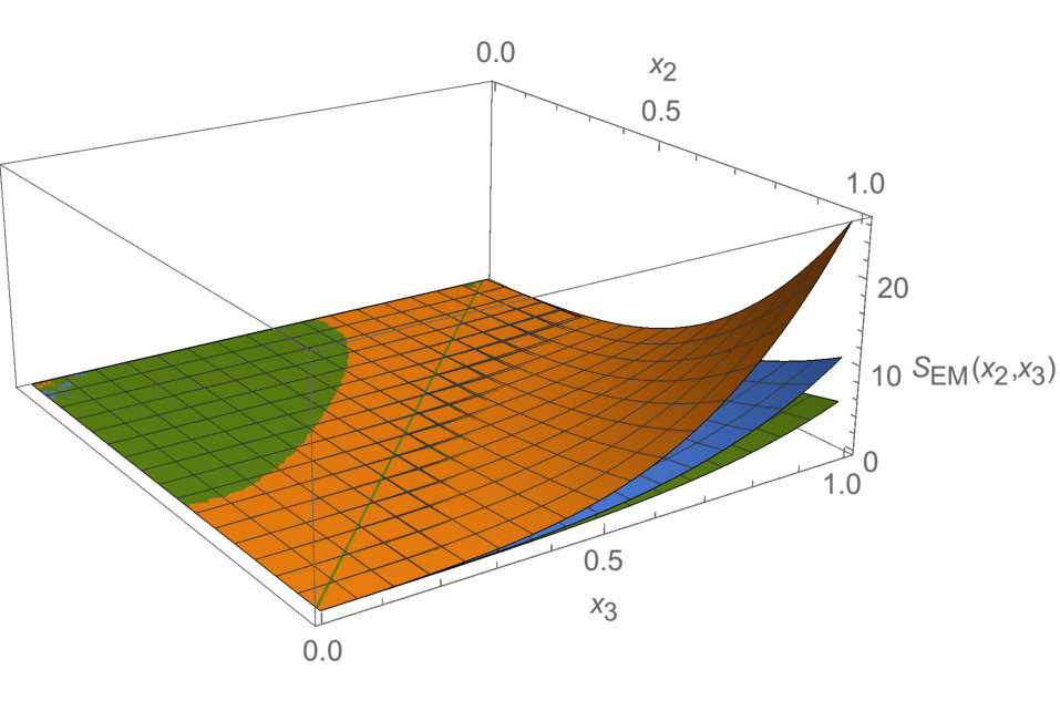 Figure 1
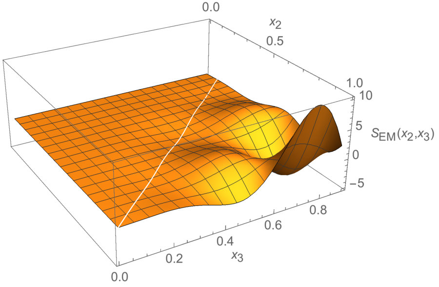 Figure 2
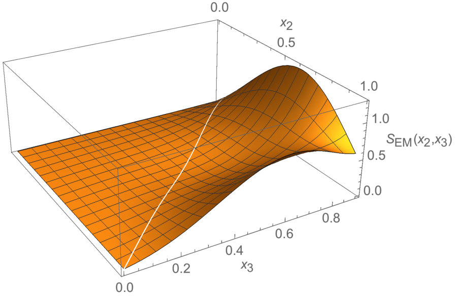 Figure 3
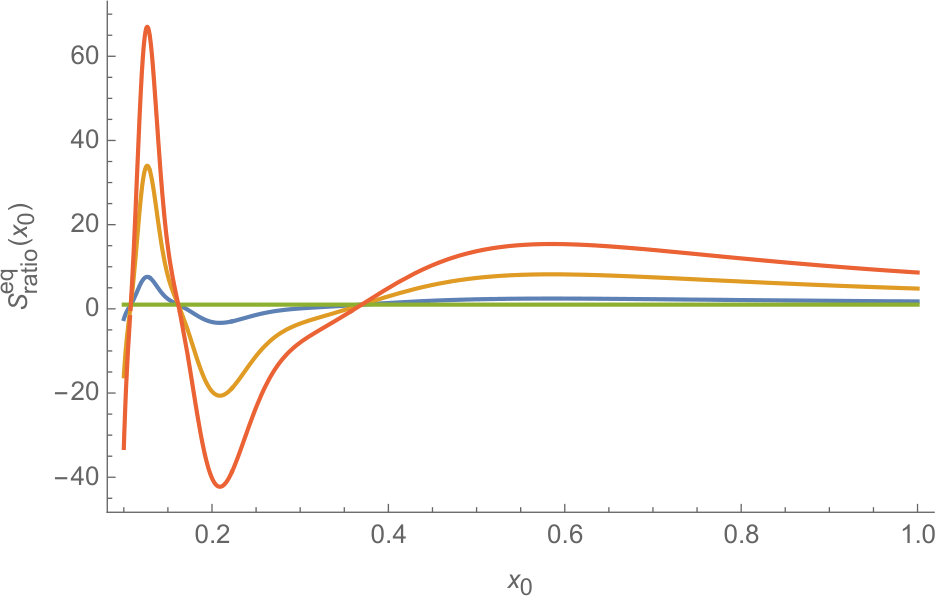 Figure 4
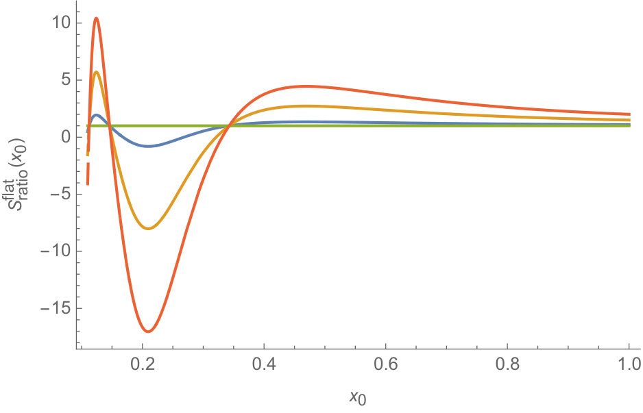 Figure 5
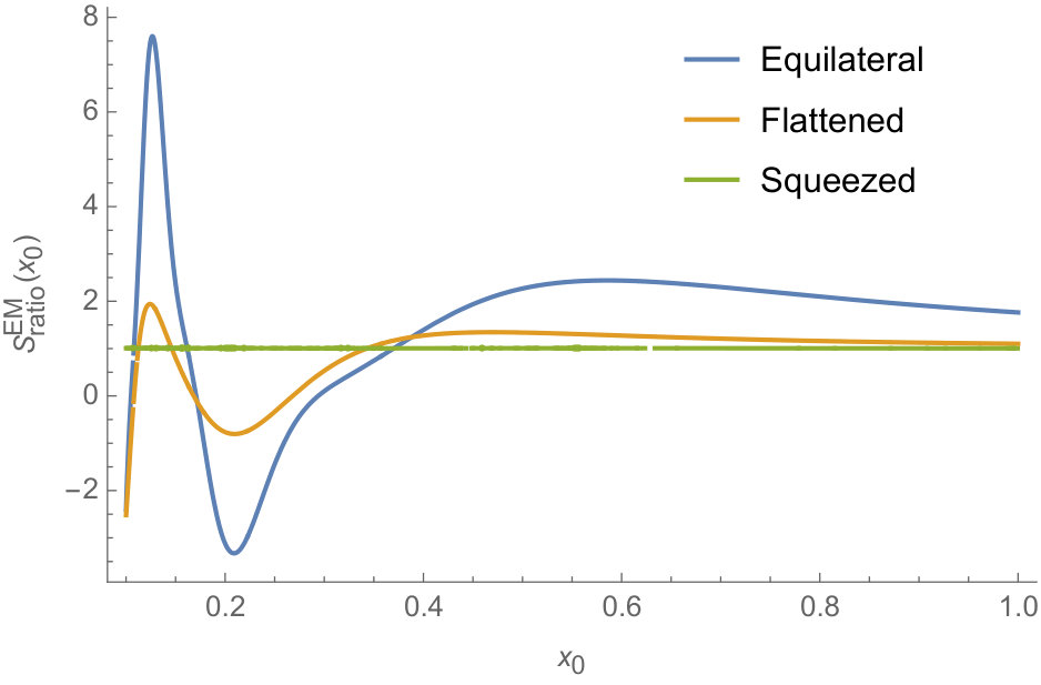 Figure 6
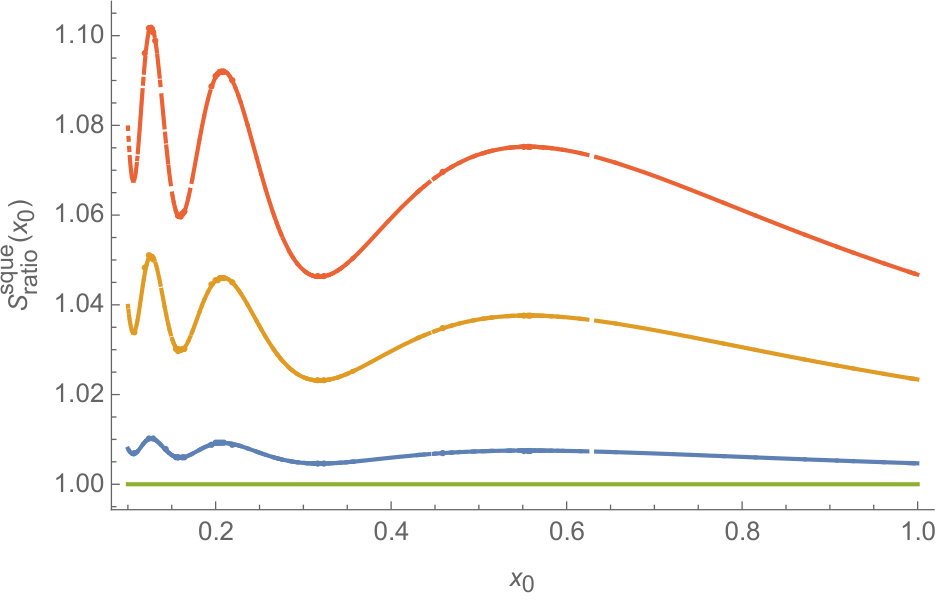 Figure 7
Peer Reviews
No public reviews on file for this paper yet. If you reviewed it on a platform where reviews are public (OpenReview, ICLR, NeurIPS, ICML), you can paste yours below so the community can read it here.
Videos
No videos yet. Explain this paper in a talk, walkthrough, or lecture? Add one.
Non-Gaussianity from Entanglement During Inflation
Nadia Bolis
Andreas Albrecht
R. Holman
Abstract
We compute the bi-spectrum of CMB temperature fluctuations for a state where the metric perturbation is entangled with a spectator scalar field . Novel terms in the cubic action coupled to the scalar can be the dominant contribution to the bi-spectrum for such states and we highlight the differences between this result and the no-entanglement bi-spectrum. New shapes can be important in the bi-spectra leading to distinctive observational signatures.
1 Introduction
A sufficient amount of cosmic inflation will expand microscopic features of the state of the universe to all observable scales. The canonical assumption, that on small scales the initial state of inflation is described by the Bunch-Davies (BD) vacuum, has produced extremely successful predictions [1]. In [2] we have advocated the use of cosmic inflation as a probe of the properties of the initial state ("the most powerful microscope in the Universe"), and showcased specific possible deviations for the BD vacuum due to quantum entanglement which could be tested in this manner.
Entangled states involve allowing other fields, such as spectator scalars[3] or tensor metric perturbations[4] to become entangled with the scalar fluctuations in the quantum state. A generic effect of such entanglement is the inducing of oscillations in the various power spectra of the CMB which are already well constrained by current data[5, 6]. A possible origin of such entangled states is discussed in [7, 8].
In prior work [3, 4] we calculated the predictions at the level of power spectra for various examples of initial state entanglement and found interesting signatures which may already be present in subtle features of the data (a more systematic analysis is underway [9]).
The power spectrum is mainly a probe of the linearized sector of field fluctuations. It can also probe interactions at loop level, although these effects will typically be suppressed. To understand the interacting aspects of the theory and to have a chance to lift the degeneracies between different inflationary models, we need to compute higher point functions, such as the bi and tri spectra. Data on these correlation functions has been gathered from both the CMB and large scale structure (LSS). While LSS non-Gaussianity data has great potential for improvements [10], CMB data, in particular from the Planck collaboration [11], provides us the best bounds to date.
In this paper we determine the shape of the bi-spectrum produced by entanglement during inflation and compare it to the no-entanglement BD bi-spectrum. We also find that the shape produced by entanglement differs from both the shape produced by an alternative non-BD model [12] (for non-Gaussianity produced by other models with an excited state or extra degrees of freedom see [13, 14, 15, 16]) and that of many multi-field inflation models (i.e local shape)[17]. Part of what drives this difference is the fact that there are new cubic operators contributing to the bi-spectrum that would not have contributed for the BD state. These operators are of the schematic form with various operators appearing. These contribute because the state now depends on the spectator scalar field through entanglement, and the contribution is proportional to the number of scalar fields. Thus, these operators can give rise to new shapes and can be made to dominate over the operators giving the standard contribution to the bi-spectrum. We also find that the magnitude of the bi-spectrum for entangled states depends on how long inflation lasted. Non-BD states typically suffer from a back-reaction problem due to the energy density of what can be thought of as particles built upon the BD vacuum. The longer the inflationary period, the larger this effect and hence there is a strong motivation to stay near the minimal number of e-folds needed to solve the horizon and flatness problems. The same principle holds for this model of entanglement and therefore, this may provide natural limits to how strong the enhancements can be.
In section 2 we first give a brief review of the construction of entangled states using the field theoretic Schrödinger picture in the Gaussian approximation. We then extend this method to allow for cubic deviations from Gaussianity. We use cosmological perturbation theory, in the presence of the relevant cubic Hamiltonians, to compute the bi-spectrum in terms of the cubic coefficient functions of the Schrödinger wavefunctional.
In section 3 we follow this use of cosmological perturbation with a second perturbative expansion in the entanglement strength parameter. This parameter is necessarily constrained to be small from observations of the CMB power spectrum so that a perturbative approach is valid here.
In section 4 we present the resulting bi-spectrum generated by these extra terms and the entanglement. We plot the shape function of this bi-spectrum and look at its equilateral, flattened and squeezed triangle limits. In section 5 we present our conclusions.
2 Entanglement in the Schrödinger Picture
The entangled states we use in this work[3] are best understood within the Schrödinger picture field theory formalism. Here we think of a wave-functional which gives the probability amplitude for finding the scalar metric perturbation and spectator field configurations on the spatial hypersurface specified by the conformal time . Note that in this formalism, are time independent; denotes the slot for the spatial variables. To compute observables we first solve the Schrödinger equation for and then use this wave-functional to compute expectation values.
2.1 The Gaussian Approximation
We recapitulate the discussion in ref [3] using the continuum momentum space rather than the box normalized one used previously.
Much as any other non-trivial quantum mechanics problem, we start from the exactly soluble Gaussian problem of the free theory and then perturb around it. The quadratic action for the - system is:
[TABLE]
where is the scale factor, , is the slow-roll parameter and is the sound speed of metric perturbations. From this we find the canonically conjugate momenta and the quadratic Hamiltonian:
[TABLE]
[TABLE]
where we’ve decomposed the fields into spatial momentum modes in the second equation:
[TABLE]
and likewise for .
The Gaussian ansatz we use that allows for entanglement between and is:
[TABLE]
where our notation in general is:
[TABLE]
Inserting this ansatz into the Schrödinger equation , using the following commutation relations:
[TABLE]
to identify (and likewise for ) and matching powers of the modes yields[3]:
[TABLE]
We have defined and likewise for the other kernels. We have also made use of the fact that rotational invariance dictates that these kernels will only depend on the magnitude of . Note the appearance of in the equation for the normalization factor; this is the comoving volume of the spatial box we quantize the system in. We can neglect this by dividing by the normalization factor when calculating observables.
The equations for the kernels are Riccatti type equations and can be converted from a set of non-linear first equations to linear second order ones. Setting
[TABLE]
with the definition of . Doing this converts eqs.(2.1) into
[TABLE]
where .
We can solve the equation for the entanglement kernel : . The parameter measures the entanglement strength and as shown in ref [3], requiring to be normalizable, implies . Consistency with CMB data would likely also require , and we will make use of this to simplify the calculation of the bi-spectrum by expanding the modes in a series of . We see from eqs.(2.1) that the leading correction to the modes due to entanglement is of order . The same is true of the two point functions calculated from :
[TABLE]
Note that the cross field correlator is linear in and vanishes when there is no entanglement.
2.2 Beyond the Gaussian Approximimation
To compute the three point function in the Schrödinger theory, we need to go beyond the Gaussian approximation of the previous subsection. The appropriate tool for this task is Schrödinger perturbation theory.
We take the Hamiltonian to be of the form: , where consists of terms in the full - action that are of cubic order in the fields. The contribution to is that calculated originally in ref.[18] and generalized to Horndeski theories in ref.[19]. There are also terms consisting of one power of and two of as in refs.[23, 24]. The parameter serves as the expansion parameter controlling the perturbative approximation. It can be made more explicit via arguments such as those in ref.[20], but we leave its exact specification open for now.
Following the ideas in ref.[21], we generalize the Gaussian wave-functional to allow for a non-trivial three-point function:
[TABLE]
where we again use the abbreviated momentum integral notation of eq.(2.6). The sum over in accounts for each of the three momenta matched with a given mode:
[TABLE]
The ’s are symmetric in the momenta corresponding to the two modes it multiplies and likewise for and the modes. The kernels are fully symmetric in their momentum arguments.
We now fix the various kernels in using perturbation theory with acting as a perturbation on top of the quadratic Hamiltonian . The parameter serves as the expansion parameter and we solve the Schrödinger equation order by order in :
[TABLE]
If we use the Schrödinger equation for we can rewrite that for as
[TABLE]
Using our expressions for in eq.(2.2) as well as that for the quadratic Hamiltonian, we find the following set of equations for the kernels:
[TABLE]
where and are the source terms derived from that correspond to each given combination of field modes.
There are two cubic Hamiltonians that contribute to the source term . First, the cubic Hamiltonian for , which can be calculated from the cubic order action [22]:
[TABLE]
Using the conjugate momenta in eq.(2.2), the cubic Hamiltonian is:
[TABLE]
where we have symmetrized the mixed conjugate momentum and terms. We also choose to take for simplicity so the first two terms from the action vanish.
The second Hamiltonian does not contribute to the BD bi-spectrum but is relevant here. It involves interaction terms that are schematically of the form [23, 24]. Their explicit form is:
[TABLE]
These will contribute to source terms for the cubic kernels, which in turn will contribute to the bi-spectrum. These terms can dominate over pure terms due to the fact that they are proportional to the number of scalars present; because of this, and the fact that their contributions to the bi-spectrum are qualitatively different from the BD ones, we will focus our attention on these terms in the remainder of this paper.
2.3 The Schrödinger Picture Approach to Calculating the Bi-spectrum
In this subsection we introduce the Schrödinger picture approach to calculating the bi-spectrum. This is a novel use of Schrödinger field theory. It gives the same answer as the interaction picture calculation[18], but generalizes to states such as the entangled one used here in a more intuitive way than is possible in the interaction picture.
The entangled three-point function is defined by taking the expectation value of using the entangled cubic state of eq.(2.2):
[TABLE]
where is defined in eq.(2.2) and the Gaussian probability density is
[TABLE]
Performing the functional integrals over the complex fields we get:
[TABLE]
where we only keep the lowest order term in the expansion parameter and denotes the real part of the various kernels. Note that has contributions from the spectator field term () and the mixed terms () and () thanks to the powers of the entanglement kernel multiplying each of them. If the entanglement vanishes, i.e. , we recover the standard BD bi-spectrum.
3
The Bi-Spectrum in the small entanglement strength limit
Solving the equations for the kernels in the cubic wavefunction is generally a difficult undertaking. On the other hand, the fact that the BD state does give an extraordinarily accurate description of the CMB power spectrum tells us that the deviations from the BD state should be small. We make use of this fact to simplify our calculations by perturbing in the entanglement parameter and keeping only the lowest non-trivial order result for the expectation value in eq.(2.25).
We start by expanding the mode functions found from the quadratic wavefunctional in terms of as dictated by the right hand side of the mode equations in eq.(2.1), since . We thus write
[TABLE]
The equations for the cubic kernels can be simplified by making the following change of variables:
[TABLE]
where and mode functions are related to each other by where and .
Using eqs.(3.2)-(3.3) the equations of motion for the cubic kernels simplify to:
[TABLE]
The superscripts in the source terms indicate the power of associated with that source term (see Appendix A for the explicit form). When there is no entanglement, i.e. the only two kernels that have a source term generated by their respective cubic Hamiltonians at zeroth order in are and , while and will vanish at this order111Note, however, that while the source term for () does not vanish when there is no entanglement, it will no longer contribute to the bi-spectrum since it is multiplied by the entanglement parameter as can be seen in eq.(2.25). In this case it will only contribute to the bi-spectrum.:
[TABLE]
We can then expand in powers of :
[TABLE]
where, without loss of generality, we have set and to satisfy the relations above.
Using these expansions in eqns.(3.4)-(3.7) and matching powers of yields a series of equations for the entanglement part of the cubic coefficients (). Each order can be found by integrating over the solutions of the previous order:
[TABLE]
Here we have only included the terms that will contribute up to overall in the bi-spectrum.
Next, we expand the bi-spectrum in eq.(2.25) in orders of the entanglement parameter . The real part of the quadratic coefficients are[3]:
[TABLE]
where each mode function is expressed in terms of its magnitude and -dependent phase . Using these, the bi-spectrum of eq.(2.25) can be rewritten:
[TABLE]
where and again, denotes the real part of each coefficient. Using our expansion of the mode functions in powers of , we can deduce the form of the leading correction to the BD bi-spectrum:
[TABLE]
At zeroth order the kernel reproduces the standard BD bi-spectrum. At quadratic order in , we see contributions coming from the higher order term as well as the mixed field kernels and . As previously mentioned, each scalar field contributes a copy of the and terms so that in the limit of large numbers of scalars (which do not have to be that large as we will see below) they will dominate. We will therefore focus on these contributions for the remainder of the paper.
4 The Shape of the Entangled Bi-Spectrum
We are now in a position to compute the 3-point function taken in the entangled state, turn this into the bi-spectrum, which in its turn can be compared to the data obtained by the Planck satellite[11].
Using the homogeneity and isotropy of the FRW background, the bi-spectrum can be expressed as follows,
[TABLE]
where is the dimensionless power spectrum evaluated at the end of inflation, and is the shape function of the bi-spectrum. One final simplification can be used if the power spectrum is scale invariant (or nearly scale invariant). In this case, the shape function only depends on ratios of the magnitudes of the momenta:
[TABLE]
In practice, when comparing to data, the bi-spectrum of a particular inflationary model has to be matched to a shape template. From a computational perspective, the easiest shapes to match to are those that can be factorized into separate functions for each of the momenta. This requirement can be relaxed at the cost of making the comparison more computational expensive.
The most standard templates are the equilateral (), local, which is maximized in the squeezed limit (), and flattened () triangle shapes. Other more complex templates for oscillatory and feature models have also been used in analyzing the Planck data [11].
As a first step, it is useful to look at one or more of the three triangle limits (equilateral, squeezed and flattened), as a way to ascertain if the bi-spectrum in question exhibits enhancements in any of these. Different enhancements in one or more of these limits can help distinguish different models of inflation and indicate which templates might be most effective to use.
In what follows we will start by plotting the entangled shape function and compare it to the no-entanglement scenario. Then we will look more closely at the equilateral, flattened and squeezed limits of the entangled bi-spectrum. Generally, non-BD models will produce enhancements in the flattened limit as well as the squeezed limit [25, 26], and multi-field inflation models are usually characterized by large enhancements in the squeezed limit. Looking at these limits will therefore give us a first glance on possible distinguishing features between these models.
In figures 1-2 we show plots of the shape function of the entangled bi-spectrum computed to ), and compare it to the no-entanglement BD shape. The shape function coming from the mixed Hamiltonian is:
[TABLE]
where is the shape function for the no-entanglement part, the subscript denotes the entangled-mixed contribution to the bi-spectrum composed by the and , the third and fourth line of the bi-spectrum in eq.(3). Note that these terms are proportional to the number of spectator scalar fields . In fig.1 from bottom to top we have the no-entanglement BD shape (green), the entangled mixed shape for one scalar field (blue) and the same for 4 spectator fields (orange). For the purpose of comparison between these scenarios we have plotted all terms proportional to slow roll parameter . Increasing the number of spectator fields can substantially increase the enhancements compared to the standard, no-entanglement scenario. These plots were done for a fixed value of . Since both the number of spectator fields and the entanglement parameter multiply the new portion of the bi-spectrum, these two parameters are partially degenerate when varied over. However, since , enhancements that correspond to a larger combined value of can indicate the presence of multiple spectators in this scenario.
The largest enhancement is in the equilateral limit. However the extra terms also contribute to the squeezed and flattened limits as will be shown in the next subsection.
The finite time integral introduces a new scale , which corresponds to the wavenumber that exits the horizon at the time entanglement turns on: ( i.e. ). The corresponding dimensionless ratio is . In what follows, corresponds to the minimal amount of entangled inflation, such that entanglement begins when the first visible modes exit the horizon. As decreases the period of entanglement increases, and finally the limit where , corresponds to eternal inflation. We will see that, as expected, taking will introduce divergences in the bi-spectrum. In fig. 2 we show plots of the entangled mixed bi-spectrum eq.(4.3) for different initial entangling times: . As the length of entangled inflation is extended, the shape of the bi-spectrum starts acquiring oscillatory features which could help put a bound on . Note however, as discussed in [3] entangled inflation cannot be extended arbitrarily since it would cause divergences in the energy density.
4.1 Equilateral, Flattened and Squeezed Limits
In this subsection we look at the three triangle limits described above: equilateral, flattened and squeezed. The , as well as , portion of the entangled bi-spectrum have terms proportional to:
[TABLE]
where is some power. At first glance it may look as though these terms will diverge in the flattened and squeezed limits, as and . In practice, such divergences arise when assuming a non-BD state back to the infinite past ; in other words, if we take the limit of the bi-spectrum integrals to be . However, realistically the entanglement behavior (or any non-BD state effect) cannot be pushed back to the infinite past, and therefore there should be a cutoff at large momenta where the entangled state is no longer valid and must be replaced. One way of implementing this is by setting the bi-spectrum integration limits to starting from some finite time when entanglement begins. This finite integration exactly cancels out the divergences that would otherwise arise in the flattened and squeezed limits. An example of such a term in the kernel is:
[TABLE]
where this can be seen explicitly; the exponential factor from the finite time integration regulates this term, allowing the flattened and squeezed limits to be finite. This differs from other non-BD models [25] and some multifield models which have large enhancements in flattened and squeezed limits, and may help distinguish between these differing models.
While all the integrals are finite, the extra terms generated by entanglement will induce enhancements in both the flattened and squeezed limits. In fig.4 we show examples of the flattened222In this plot we chose the flattened limit where as an illustrative example. (a) and squeezed (b) limit of the ratio of the entangled bi-spectrum shape and the no-entanglement BD shape function , for all initial entangling scales . The enhancements, compared to the standard scenario, are generally larger for the flattened limit rather then the squeezed limit for a given number of spectator fields. As mentioned above largest enhancements, however, are in the equilateral limit as can be seen in fig.3, with the three triangle limits compered directly in plot (a) and with the equilateral limit for multiple spectator fields in plot (b).
It is plausible that a full comparison of this entanglement model with current data could result in tight constraints on the entanglement strength parameter and number of spectator fields . We reserve a full analysis and comparison with data to future work.
5 Conclusion and Discussion
In this work we calculated the bi-spectrum produced by entanglement between the curvature perturbations and a spectator scalar field during inflation. The bi-spectrum captures the higher order interactions of a theory and therefore can help further distinguish between inflationary models.
Using the field theoretic Schrödinger picture to describe the entangled state required the use of Schrödinger perturbation theory to calculate the corrections to the 3-point function. We found that terms in the cubic Hamiltonian that involve mixing between the spectator field and were the most interesting ones to focus on, not least due to the fact that the effect they generate on the three point function can be enhanced by having many scalars entangle with the curvature perturbation.
We argued that the entangled bi-spectrum shape, computed to first order in , differs from the non-BD model and the local shape non-Gaussianity typical of many multi-field models. In particular while these shapes differ moderately with respect to the short entangled inflation shape, more complex oscillatory shapes arise as entanglement is extended to the far past.
To further gain some intuition about the behavior of the entangled bi-spectrum we also looked at the equilateral, flattened and squeezed limits. In all three cases entanglement induces enhancements to the signal, with the largest being in the equilateral limit. The larger the entanglement parameter the larger the over all enhancement. Varying the length of entangled inflation will also affect the magnitude of these enhancements. For shorter entangled inflation () the enhancements, for values of that are not visibly excluded by angular power spectrum data (), get no larger then two times the BD bi-spectrum value in the case with one spectator field. However, for longer entangled inflation, and/or more spectator fields, the enhancements increase and could be used to exclude long entangled inflation and put a bound on the allowed number of entangled fields. In a full analysis to constrain this model, the effect of the tensor to scalar ratio (and other relevant cosmological parameters) will also have to be taken into account.
The enhancement and features that appear in the entangled bi-spectrum shape can serve as a way to distinguish between this model and similar models, in a complementary way to the use of the angular power spectrum.
We conclude that the bi-spectrum provides an interesting set of new signals that expands the opportunities to test the initial state entanglement ideas beyond the signatures already explored in the power spectra [3, 4]. These new signals allow us to further advance the goals of using inflation as “the most powerful microscope in the Universe” [2] to explore the nature of the initial state.
Acknowledgments
NB acknowledges funding from the European Research Council under the European Union’s Seventh Framework Programme (FP7/2007-2013)/ERC Grant Agreement No. 617656 “Theories and Models of the Dark Sector: Dark Matter, Dark Energy and Gravity. AA thanks Department of Energy Grant DE-SC0019081 and UC Davis for support. RH thanks the Center for Quantum Mathematics and Physics and the Physics Department at UC Davis for hospitality while this work was in progress.
Appendix A Source terms at each order in the entanglement
Grouping together for each power of the source terms generated by acting the and cubic Hamiltonian on the Gaussian entangled state gives:
[TABLE]
The zeroth order sources and don’t have any entanglement kernels , the first order source is proportional to one power of and the second order source has two powers of .
The reference list from the paper itself. Each links out to its DOI / PubMed record.
- 1[1] P. A. R. Ade et al. [Planck Collaboration], Astron. Astrophys. 594 , A 13 (2016) doi:10.1051/0004-6361/201525830 [ar Xiv:1502.01589 [astro-ph.CO]].
- 2[2] A. Albrecht, N. Bolis and R. Holman, “Cosmic Inflation: The Most Powerful Microscope in the Universe,” ar Xiv:1806.00392 [hep-th].
- 3[3] A. Albrecht, N. Bolis and R. Holman, “Cosmological Consequences of Initial State Entanglement,” JHEP 1411 , 093 (2014) [ar Xiv:1408.6859 [hep-th]].
- 4[4] N. Bolis, A. Albrecht and R. Holman, “Modifications to Cosmological Power Spectra from Scalar-Tensor Entanglement and their Observational Consequences,” JCAP 1612 , no. 12, 011 (2016) Erratum: [JCAP 1708 , no. 08, E 01 (2017)] [ar Xiv:1605.01008 [hep-th]].
- 5[5] P. A. R. Ade et al. [Planck Collaboration], “Planck 2015 results. XX. Constraints on inflation,” Astron. Astrophys. 594 , A 20 (2016) [ar Xiv:1502.02114 [astro-ph.CO]].
- 6[6] Y. Akrami et al. [Planck Collaboration], “Planck 2018 results. X. Constraints on inflation,” ar Xiv:1807.06211 [astro-ph.CO].
- 7[7] N. Bolis, T. Fujita, S. Mizuno and S. Mukohyama, “Quantum Entanglement in Multi-field Inflation,” JCAP 1809 , 004 (2018) [ar Xiv:1805.09448 [astro-ph.CO]].
- 8[8] R. Holman and B. J. Richard, “Generating Entangled Inflationary Quantum States,” ar Xiv:1902.00521 [hep-th].