Cohomological invariants of representations of 3-manifold groups
Haimiao Chen

TL;DR
This paper introduces a cohomological invariant for representations of 3-manifold groups, extending its definition to manifolds with corners, and provides a practical computation method, including for the Chern-Simons invariant.
Contribution
It extends the invariant to manifolds with corners and develops a gluing law, enabling practical computation from link surgery presentations.
Findings
Defined a cohomological invariant for 3-manifold group representations.
Extended the invariant to manifolds with corners.
Provided a method to compute the invariant via link surgery, including the Chern-Simons invariant.
Abstract
Suppose is a discrete group, and , with an abelian group. Given a representation , with a closed 3-manifold, put , where is a continuous map inducing which is unique up to homotopy, and is the pairing. We extend the definition of to manifolds with corners, and establish a gluing law. Based on these, we present a practical method for computing when is given by a surgery along a link . In particular, the Chern-Simons invariant can be computed this way.
Click any figure to enlarge with its caption.
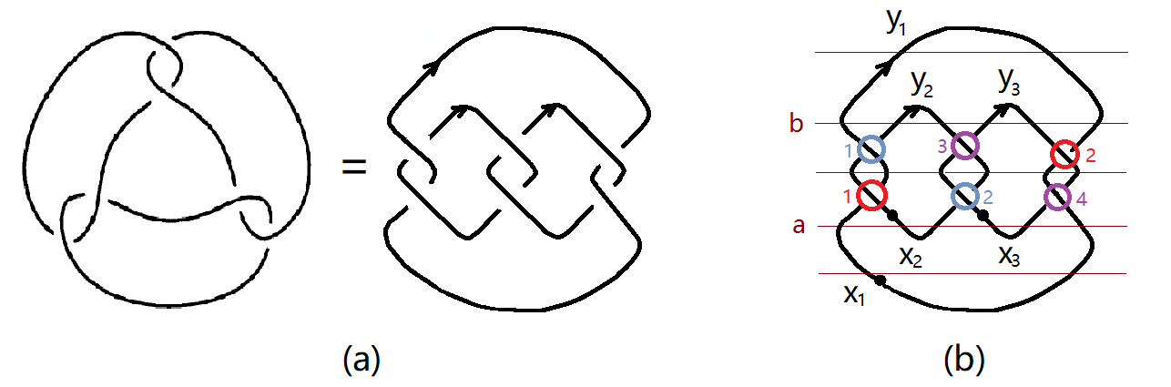 Figure 1
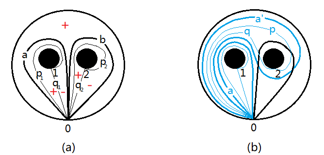 Figure 2
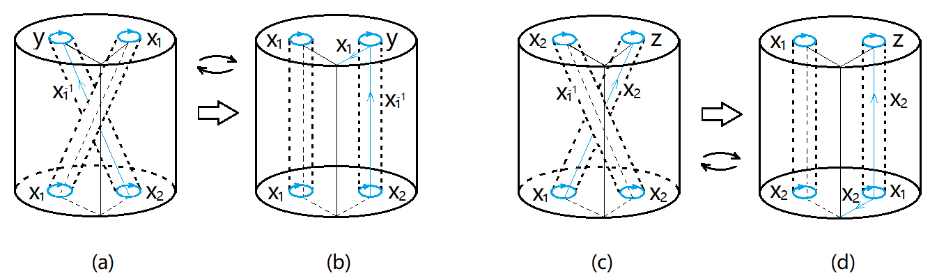 Figure 3
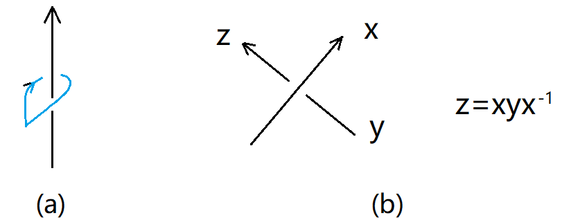 Figure 4
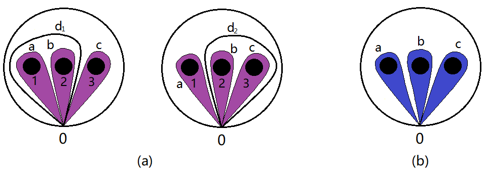 Figure 5
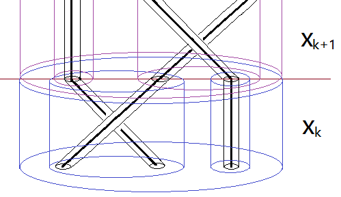 Figure 6
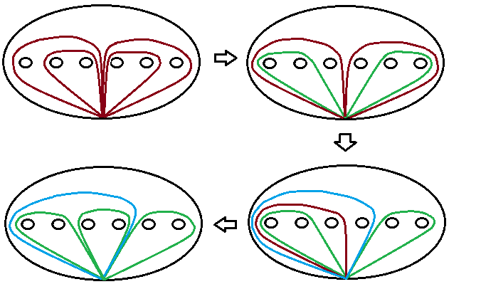 Figure 7
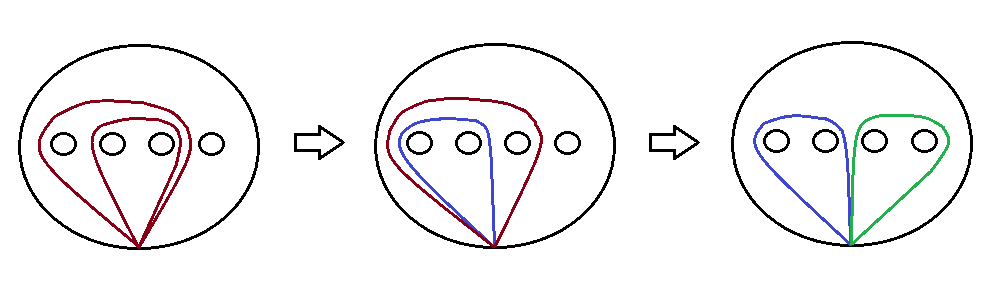 Figure 8
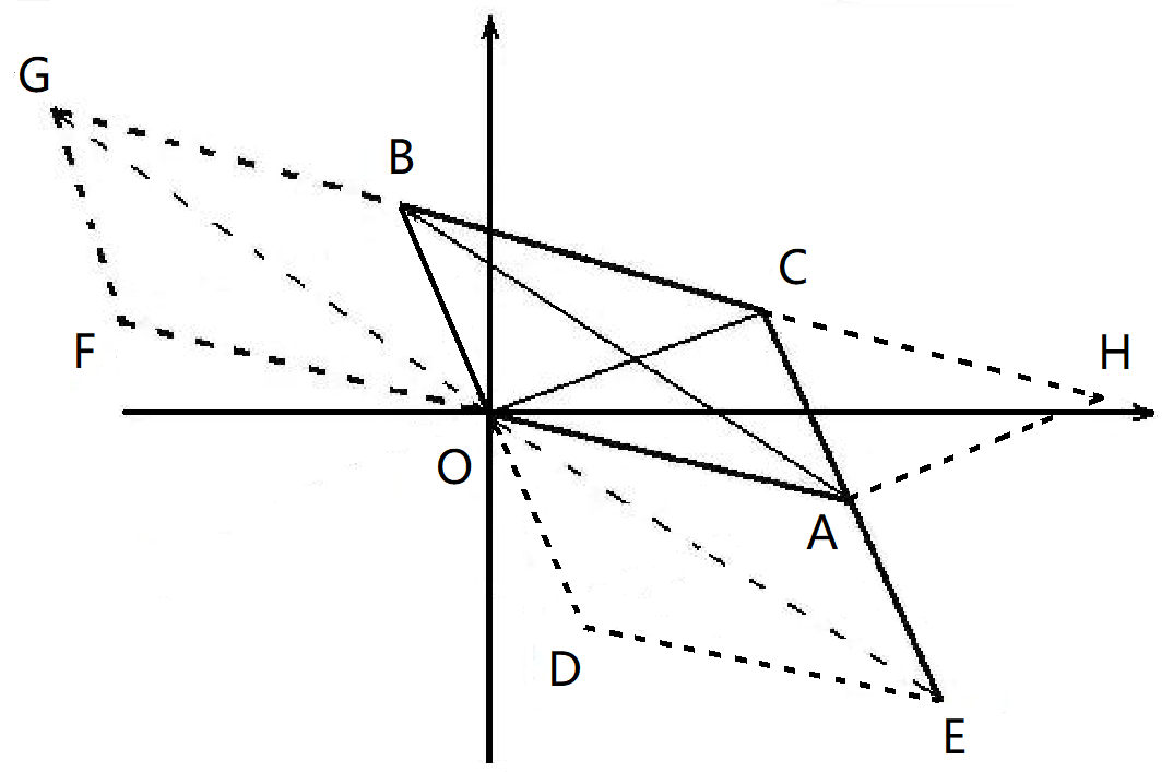 Figure 9
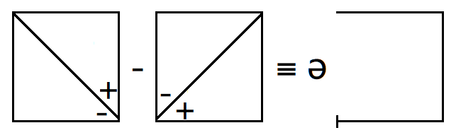 Figure 10
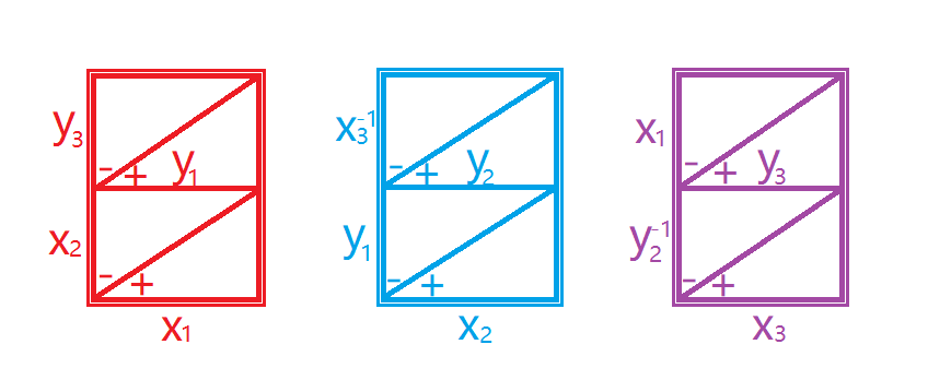 Figure 11
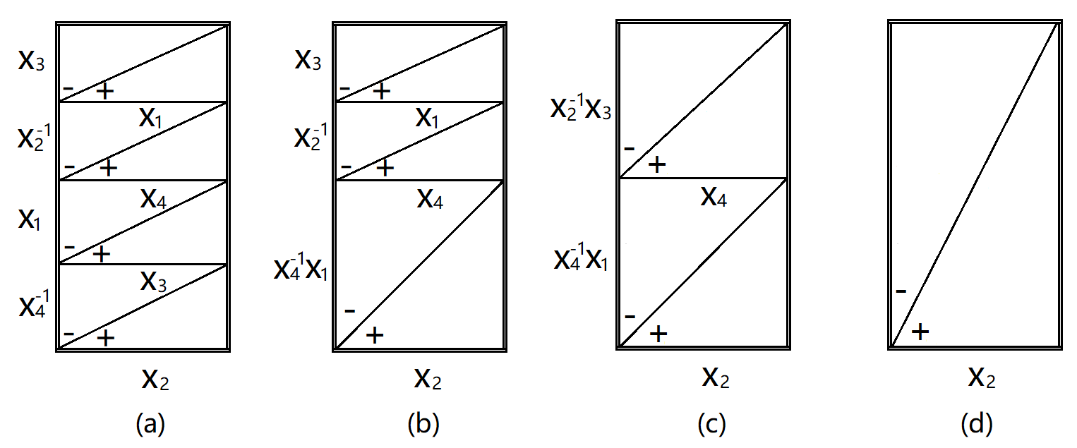 Figure 12
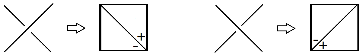 Figure 13
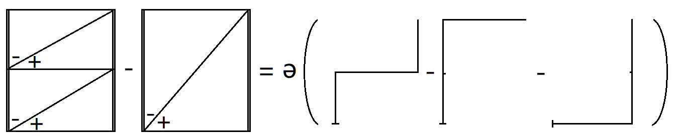 Figure 14
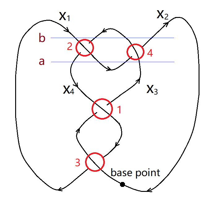 Figure 15
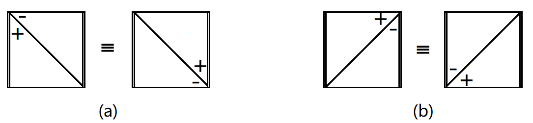 Figure 16
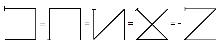 Figure 17
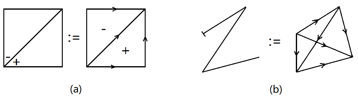 Figure 18
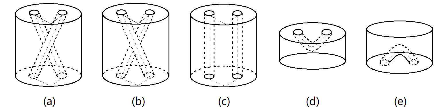 Figure 19
Peer Reviews
No public reviews on file for this paper yet. If you reviewed it on a platform where reviews are public (OpenReview, ICLR, NeurIPS, ICML), you can paste yours below so the community can read it here.
Videos
No videos yet. Explain this paper in a talk, walkthrough, or lecture? Add one.
Taxonomy
TopicsGeometric and Algebraic Topology · Homotopy and Cohomology in Algebraic Topology · Algebraic structures and combinatorial models
Cohomological invariants of representations of 3-manifold groups
Haimiao Chen 111Email: [email protected]
Mathematics, Beijing Technology and Business University, Beijing, China
Abstract
Suppose is a discrete group, and , with an abelian group. Given a representation , with a closed 3-manifold, put , where is a continuous map inducing which is unique up to homotopy, and is the pairing. We extend the definition of to manifolds with corners, and establish a gluing law. Based on these, we present a practical method for computing when is given by a surgery along a link . In particular, the Chern-Simons invariant can be computed this way.
Keywords: cohomological invariant, 3-manifold, fundamental group, representation, Chern-Simons invariant
MSC 2020: 57K31
1 Introduction
Suppose is a discrete group, and , with an abelian group. Given a representation , with a closed 3-manifold, put
[TABLE]
where is a continuous map inducing which is unique up to homotopy, and is the pairing. It is a subtle problem to define when , and will be handled in this paper.
There are at least two reasons for us to care about this cohomological invariant. First, if is a finite group and , then
[TABLE]
is by definition the Dijkgraaf-Witten invariant of associated to . Second, if and viewed as a discrete group, then for a certain representing the Cheeger-Chern-Simons class , one has that equals the Chern-Simons invariant (CSI for short) which is meant to be that of the flat connection corresponding to .
The importance of CSI is manifested in several aspects of geometry and topology; see [5, 6, 8, 9, 20] and the references therein. There have been many works in the literature on computing CSI. Zickert [21] gave a formula for boundary-parabolic -representations, for with tori boundary. Hatakenaka and Nosaka [13], Inoue and Kabaya [14] used quandle to derive a new formula for . Marché [17] filled all tetrahedra with a connection as explicit as possible, and computed the contribution of each teterhedron. Garoufalidits, Thurston and Zickert [10] gave a formula for any and . Besides, computations for concrete manifolds are seen in: Kirk and Klassen [15]; Cho, Murakami and Yokota [3]; Ham and Lee [12].
We aim to present a convenient method for computing general cohomological invariants. It is more flexible in that there needs to be no restriction on boundary.
In Section 2, we set up a general framework for , and reveal some fine structures around; in particular, we define when is a 3-manifold with boundary. This is largely based on [2] Section 2, which in turn was an exposition using algebraic notions of the construction given by Freed [7].
In Section 3, we propose a method for computing when is the complement of a link in . An efficient procedure is designed, starting from a link diagram. After that, if a closed 3-manifold is given as a surgery along a link, then can be written down. All these are in accord with the sprit of Turaev’s homotopy quantum field theory [19].
Acknowledgement
The author is supported by NSFC-11771042.
2 General framework
2.1 Preparation
Convention 2.1**.**
In this paper, all manifolds are oriented. For a manifold , let denote the one obtained by reversing the orientation of .
For a topological space , let denote the fundamental groupoid of , i.e. the category whose objects are points of and whose morphisms are homotopy classes of paths. Let , the set of functors , where is viewed as a groupoid with a single object.
Suppose is a finite subset of such that each connected component of contains at least one point from . Let be the full subgroupoid of with as the set of objects, then is equivalent to through the inclusion . There is a restriction
[TABLE]
For , abusing the notation, we denote its image in also by . In most situations in this paper, it is sufficient to consider for some .
Let denote the standard -simplex. For each singular -simplex , let and let . Abbreviate to .
Let . Given a singular -chain , put
[TABLE]
where for each singular -simplex , we set .
Let be an abelian group, for which additive notations are used, and let be a discrete group. A 3-cocycle is a function satisfying
[TABLE]
for all . Recall that (see [11] Page 89) has a simplicial model, in which -simplices are ordered -tuples with . The boundary map is given by
[TABLE]
The value of taking at is .
2.2 Extending to manifolds with boundary
Definition 2.2**.**
For an -manifold , call a singular chain an s-triangulation if represents the fundamental class . Let denote the set of s-triangulations. This is consistent with the notion of the fundamental class of when is closed.
Viewing as an -manifold, put .
Given , the meaning of is self-evident.
Let be a closed surface. For , define to be the set of the functions such that for any and with . Notice two facts: (i) for any , since and , one can find such that ; (ii) if , then , as and is a cocycle. Hence the action given by
[TABLE]
is free and transitive, so is an -torsor, as is called in the literature.
For a closed 3-manifold , take an arbitrary , and put for any . Clearly, this is in consistence with (1).
Now consider a general 3-manifold . Write , where is closed, and each connected component of has nonempty boundary. Then . Given , let and . For each , define to be for any (so that ). This is well-defined, thanks to the following: (i) such a always exists; (ii) if , then , and since , we may find with , so . Moreover, if , then taking with and putting , we have
[TABLE]
Hence indeed , with . Define
[TABLE]
Remark 2.3**.**
We highlight that to determine , it suffices to take an arbitrary and specify the value . Then the value of at any is given by , for an arbitrary with .
Lemma 2.4** (Gluing law).**
Suppose , and is an orientation-preserving homeomorphism. Let , i.e. the manifold obtained from gluing along , so that ; let denote the quotient map. Given , let , then for any and , one has
[TABLE]
Proof.
Take with , then , so
[TABLE]
∎
We must also allow manifolds to have corners. In this paper, 3-manifolds with corners are viewed as ordinary 3-manifolds together with a piece of information encoding how to decompose into subsurfaces along circles. For , we simply define as above, temporarily forgetting that has corners. A gluing rule in this more general context can be established. But it is such an easy task that we choose not to explicitly write down.
2.3 Fundamental cycle
Motivated by [18, 16, 21], we introduce a universal notion.
Given a topological space , define an equivalence relation on by declaring that two singular -simplices are equivalent if in for all , and extending linearly. Let denote the set of equivalence classes. Clearly descends to a map . Let denote the composite
[TABLE]
For a 3-manifold , define by sending to , for any with . This is well-defined: such an always exists; if also , then represents , so that for some , hence . Call the map the fundamental cycle of .
Remark 2.5**.**
Let be the inclusion. Straightforward is the property that for any and with .
For any and any , abusing the notation, there is an induced map such that the composite
[TABLE]
equals defined in the previous subsection.
2.4 Cycle-cocycle calculus
The name was given in [2], to mean the following procedure: given and , to find with and compute , which is independent of the choice of . We abbreviate to when is clear.
Convention 2.6**.**
From now on, we assume that is strongly normalized, meaning whenever , as defined in [13] Section 6.1.
Remark 2.7**.**
Such an can be found at least for the Chern-Simons invariant over (see [13] Lemma 6.4), and we expect similar results for more Lie groups.
If is not strongly normalized, then the formulas below still exist, but will be more complicated. We may develop these in future work.
Notation 2.8**.**
For , suppose there exists with . Denote (resp. ) if for all and all normalized (resp. strongly normalized) .
Convention 2.9**.**
From now on, for each manifold , write instead of , after a finite set is chosen.
For a planar surface, let consist of one vertex from each component of . For torus , let .
In Fig. 1 we introduce some pictorial notations which are used throughout this paper.
Since , we have ; similarly, . It then follows from that
[TABLE]
Consequently,
[TABLE]
as illustrated by Fig. 2.
The assumption that is strongly normalized implies the following:
[TABLE]
the second line is illustrated in Fig. 3. These are easy to deduce and will be used implicitly from now on.
2.4.1 Pair of pants
Let (resp. ) denote the clockwise loop from (resp. ) to itself. The other notations in the following lines deserve no explanation. Let
[TABLE]
Let denote the clockwise twist, under which the two holes are interchanged. The transformed s-triangulation is found to be
[TABLE]
as shown in Fig. 4 (b). Then
[TABLE]
Let be the one given by , and for , then
[TABLE]
2.4.2 Disk with at least 3 holes removed
Let be the two s-triangulations shown in Fig. 5 (a), where the inner parts in light gray are similar as those in Fig. 4 (a).
For , let send to and to for . Since
[TABLE]
we have
[TABLE]
In this manner, if , then an s-triangulation of corresponds to a vertex in the associahedron (c.f. [1]), and given two such s-triangulations , we may find with , which corresponds to a path in . Then, letting send to and to for , we can compute by successively using (9). Call this value an associator; it is independent of the choice of .
2.4.3 Cylinder
We often draw a cylinder as a rectangle with a pair of opposite edges in double lines, to indicate that they are to be identified.
Let respectively denote the four s-triangulations in Fig. 6 from left to right. As an immediate consequence of (3), we have equivalences
[TABLE]
Two cylinders can be glued into a new one: , and a 3-chain whose boundary is can be found via Rule (I) shown in Fig. 7.
2.4.4 Torus
Let be the universal covering. For , , use to denote the singular 2-simplex , where is the map extending linearly. Similarly for singular 3-simplices in .
Write elements of as column vectors. Let
[TABLE]
Recall the well-known fact that the mapping class group of is isomorphic to , which is generated by
[TABLE]
For , let denote the homeomorphism induced by the left multiplication . Then sets up an isomorphism of onto .
For each , the map , is a 3-cocycle of , so, due to , there exists such that
[TABLE]
for all . Put
[TABLE]
clearly, it is independent of the choice of .
Setting in (21), we obtain
[TABLE]
Furthermore, in (21), the case implies , the case implies , and
[TABLE]
so that . Hence
[TABLE]
Lemma 2.10**.**
Let be determined by and . Then
[TABLE]
Proof.
The result is trivial when is the identity matrix. The proof proceeds as showing: if (27) is true for , then it is also true for
[TABLE]
Let . Assuming (27), we have (as in Fig. 8)
[TABLE]
Computing directly, one obtains
[TABLE]
hence \omega^{\phi_{z}}\big{(}(\hat{\mathbf{a}}\hat{\mathbf{s}})_{\#}\xi^{\rm st}_{\mathbb{T}^{2}};\hat{\mathbf{a}}_{\#}\xi^{\rm st}_{\mathbb{T}^{2}}\big{)}=\alpha(z^{d},z^{c-d},z^{d}), which together with the assumption implies
[TABLE]
So (27) holds for .
Similarly, we can also prove (27) for , . The reader may consult the proof of Lemma 3.4 in [2]. ∎
3 A practical method for computations
The main results are Algorithm 3.2 for computing when is a link complement, and the formula (35) for when is presented as a surgery along a link.
3.1 Link complements
Let be a link, where the ’s are connected components. Take a sufficiently large solid cylinder containing the tubular neighborhood , and let , , then , where does not affect anything below. Suppose is presented as a diagram , with corresponding to , and suppose a representation is given via a coloring (where is the set of directed arcs) fitting the Wirtinger presentation for .
Convention 3.1**.**
We adopt the “over presentation” for (see [4] Chapter VI), as in Fig. 9.
Fix an orientation for . For each , fix an homeomorphism from to the , and let stand for the -th component of ; denote the image of by (the meridian), and denote that of by (the longitude); label via a big dot on some arc of and call it basepoint.
Use horizontal lines to cut into simple pieces. The corresponding 3-dimensional picture is to use horizontal planes to decompose into layers, each of which can be chopped into “basic pieces” exhibited in Fig. 10; note that for can be obtained by successively gluing copies of . Recalling Convention 2.9, choose for the finite set consisting of the vertices, one for each circle. From we can construct a representation (abusing the notation) in an self-evident way, so that when restricted to it is respectively in the form shown in Fig. 11 (a),(c).
For , as parts of its boundary, let , respectively denote the upper and lower pair of pants, let denote the outer cylinder, and the inner cylinders.
Let and be determined by the assignments shown in Fig. 11 (a), (b), respectively. Then
[TABLE]
in the last equality we use by (8), and the equality
[TABLE]
which is shown as follows: applying the “prism operator” (defined in [11] Page 112) to the homeomorphism , we get and then
[TABLE]
Hence
[TABLE]
Let and be determined by the assignments shown in Fig. 11 (c), (d), respectively. Then
[TABLE]
we have used by (8), and the equality
[TABLE]
which is obtained similarly as above, noting that the 3rd term in (7) contributes .
Furthermore, we can easily show that and contribute nothing; the details are omitted.
Now appears to be glued from small cylinders, two for each crossing. However, the one arising from the overcrossing arc can be “absorbed”, due to Rule (I). Moreover, thanks to (10), we are able to freely turn a square in a half-circle. Consequently, remembering (28), (29), we may find by gluing small cylinders, one for each crossing according to Rule (II) (as presented in Fig. 13). Then Rule (I) can be applied to compute \omega\big{(}\xi_{\mathcal{L},i};\xi^{\rm st}_{\mathbb{T}^{2}_{i}}\big{)}.
Finally remained is another issue. When decomposing into basic pieces, the two planar surfaces belonging to adjacent layers are usually triangulated differently, as illustrated in Fig. 12. These account for associators. To be precise, for the layers to be correctly glued, we must re-triangulate one of these two surfaces. Let denote the -th layer, numbered from below to up, and let , , , be the s-triangulations of the upper, lower, inner, outer boundary, respectively. We have computed , so
[TABLE]
All these are summarized to give
Algorithm 3.2**.**
For each , go ahead guided by the orientation of , and draw a small triangulated cylinder according to Rule (II) whenever passing a crossing underneath. The result when back to the basepoint is an s-triangulation of .
Use horizontal planes to decompose into layers. Let () denote the s-triangulations of the -th interface induced from the upper, lower layers, respectively.
Then F(E_{L},\rho_{c})\big{(}\sqcup_{i=1}^{n}-\xi^{\rm st}_{\mathbb{T}^{2}_{i}}\big{)}=\delta_{\mathcal{L},c}+\theta_{\mathcal{L},c}, with
[TABLE]
Example 3.3**.**
Let be the figure eight knot, for which a diagram together with a coloring is given in Fig. 14.
Referring to Fig. 15 and successively applying Rule (I), we get
[TABLE]
From Fig. 16, using (9) twice, we see that the associator at level is
[TABLE]
Similarly, . The associators at the other levels all vanish. Hence
[TABLE]
Thus equals the sum of the right-hand-sides of (31) and (32).
Example 3.4**.**
Let be the 3-chain link, which is also the -pretzel link. A diagram together with a coloring is given in Fig. 17 (b).
Referring to Fig. 18 and applying Rule (I), we obtain
[TABLE]
Referring to Fig. 19, we have
[TABLE]
Similarly, The associators at the other levels all vanish. So
[TABLE]
Now F(E_{L},\rho_{c})\big{(}\sqcup_{i=1}^{3}-\xi^{\rm st}_{\mathbb{T}^{2}_{i}}\big{)} equals the sum of the right-hand-sides of (33) and (34).
3.2 Closed 3-manifolds with a surgery presentation
Consider the closed 3-manifold resulting from a surgery along a link :
[TABLE]
where , with \mathbf{a}_{i}=\left(\begin{array}[]{cc}p_{i}&p^{\prime}_{i}\\ q_{i}&q^{\prime}_{i}\end{array}\right)\in{\rm SL}(2,\mathbb{Z}) for some integrs that are irrelevant; the -th solid torus is glued onto so that .
Given , let , and . Applying Lemma 2.4 to , and , we deduce
[TABLE]
where z_{i}=\rho\big{(}\mathfrak{m}_{i}^{p^{\prime}_{i}}\mathfrak{l}_{i}^{q^{\prime}_{i}}\big{)}, which can be characterized by and . Thus, using (27), we obtain
[TABLE]
The reference list from the paper itself. Each links out to its DOI / PubMed record.
- 1[1] C. Ceballos, F. Santos, G.M. Ziegler. Many non-equivalent realizations of the associahedron , Combinatorica 35 (2015), no. 5, 513–551.
- 2[2] H-M. Chen, The Dijkgraaf-Witten invariants of Seifert 3-manifolds with orientable bases . J. Geom. Phys. 108 (2016), 38–48.
- 3[3] J. Cho, J. Murakami, Y. Yokota, The complex volumes of twist knots . Proc. AMS. 137 (2009), no. 10, 3533-3541.
- 4[4] R.H. Crowell, R. Fox, Introduction to knot theory . Graduate Texts in Mathematics, Vol. 57, Springer-Verlage, New York, Heidelberg, Berlin, 1977.
- 5[5] T. Dimofte, S. Gukov, Quantum Field Theory and the Volume Conjecture . In: Interactions Between Hyperbolic Geometry Quantum Topology & \& Number Theory, Contemp. Math., Vol. 541, Amer. Math. Soc., Providence, RI, 2011. 41-67.
- 6[6] P. Derbez, Y. Liu, S-C. Wang, Chern-Simons theory, surface separability, and volumes of 3-manifolds . J. Topol. 8 (2015), no. 4, 933–974.
- 7[7] D.S. Freed, Higher algebraic structures and quantization . Commun. Math. Phys. 159 (1994), no. 2, 343–398.
- 8[8] D.S. Freed, Classical Chern-Simons Theory, 1 . Adv. Math. 113 (1995), no. 2, 237–303.