On the Probability Density of the Nuclei in a Vibrationally Excited Molecule
Axel Schild

TL;DR
This paper investigates the one-nucleus probability density in vibrationally excited molecules, revealing how vibrational states influence nuclear distributions and how these can be predicted and potentially observed experimentally.
Contribution
It introduces a quantum-mechanical analysis of the one-nucleus density in vibrationally excited molecules, providing rules to predict vibrational excitation visibility in experiments.
Findings
Nodes are not always visible in the one-nucleus density.
Certain vibrational excitations significantly alter the density.
Simple rules can predict the shape of the density from normal modes.
Abstract
For localized and oriented vibrationally excited molecules, the one-body probability density of the nuclei (one-nucleus density) is studied. Like the familiar and widely used one-electron density that represents the probability of finding an electron at a given location in space, the one-nucleus density represents the probability of finding a nucleus at a given position in space independent of the location of the other nuclei. In contrast to the full many-dimensional nuclear probability density, the one-nucleus density contains less information and may thus be better accessible by experiment, especially for large molecules. It also provides a quantum-mechanical view of molecular vibrations that can easily be visualized. We study how the nodal structure of the wavefunctions of vibrationally excited states translates to the one-nucleus density. It is found that nodes are not necessarily…
Click any figure to enlarge with its caption.
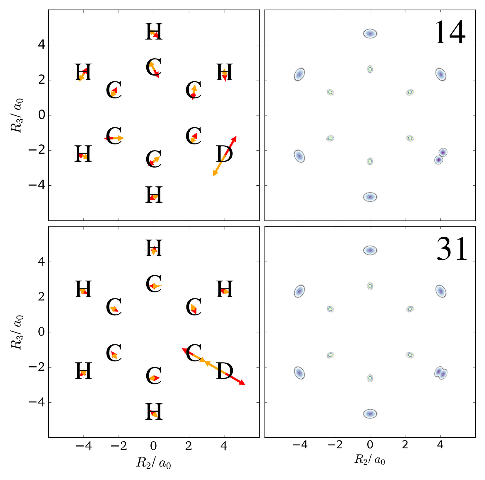 Figure 1
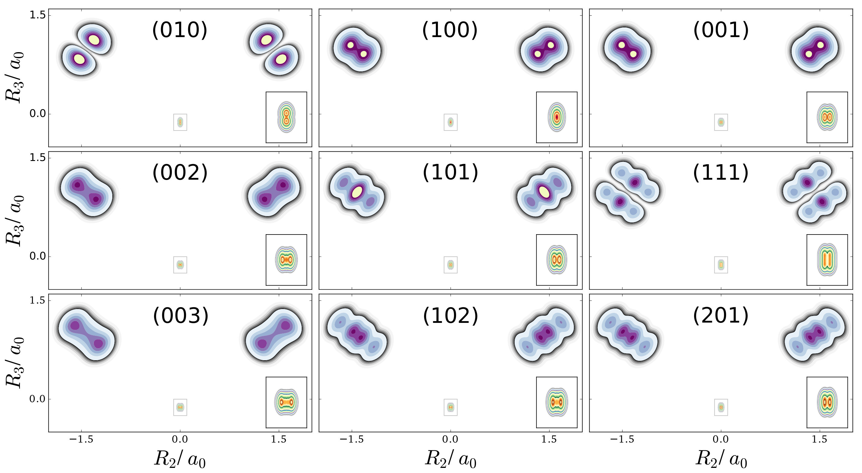 Figure 2
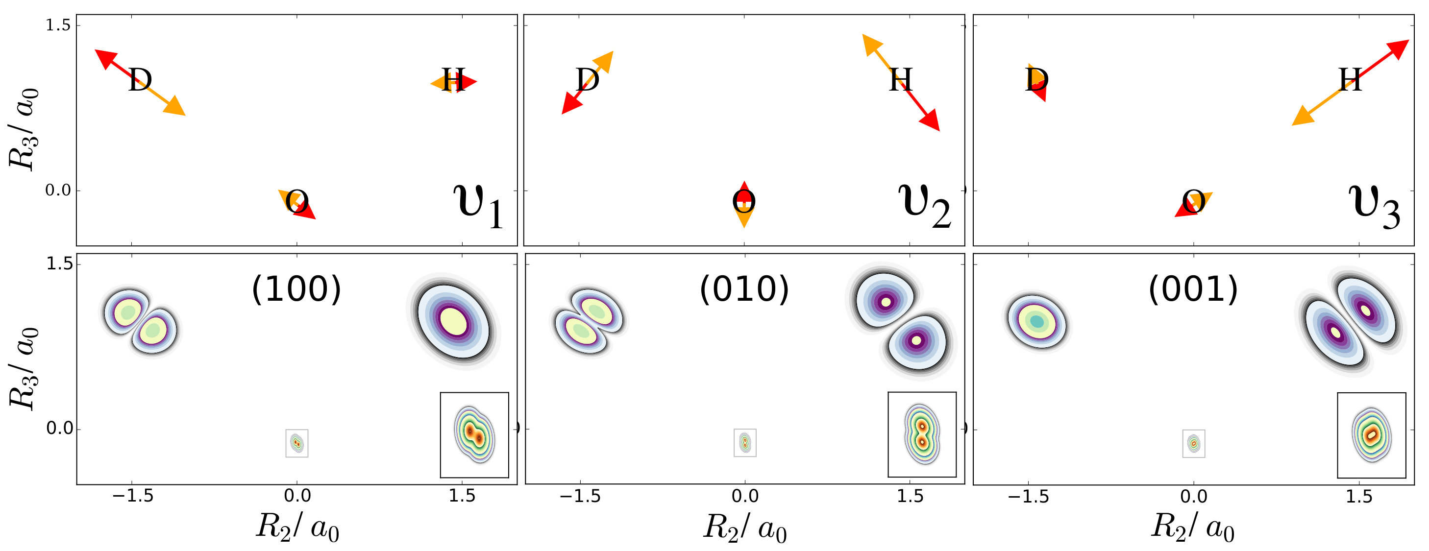 Figure 3
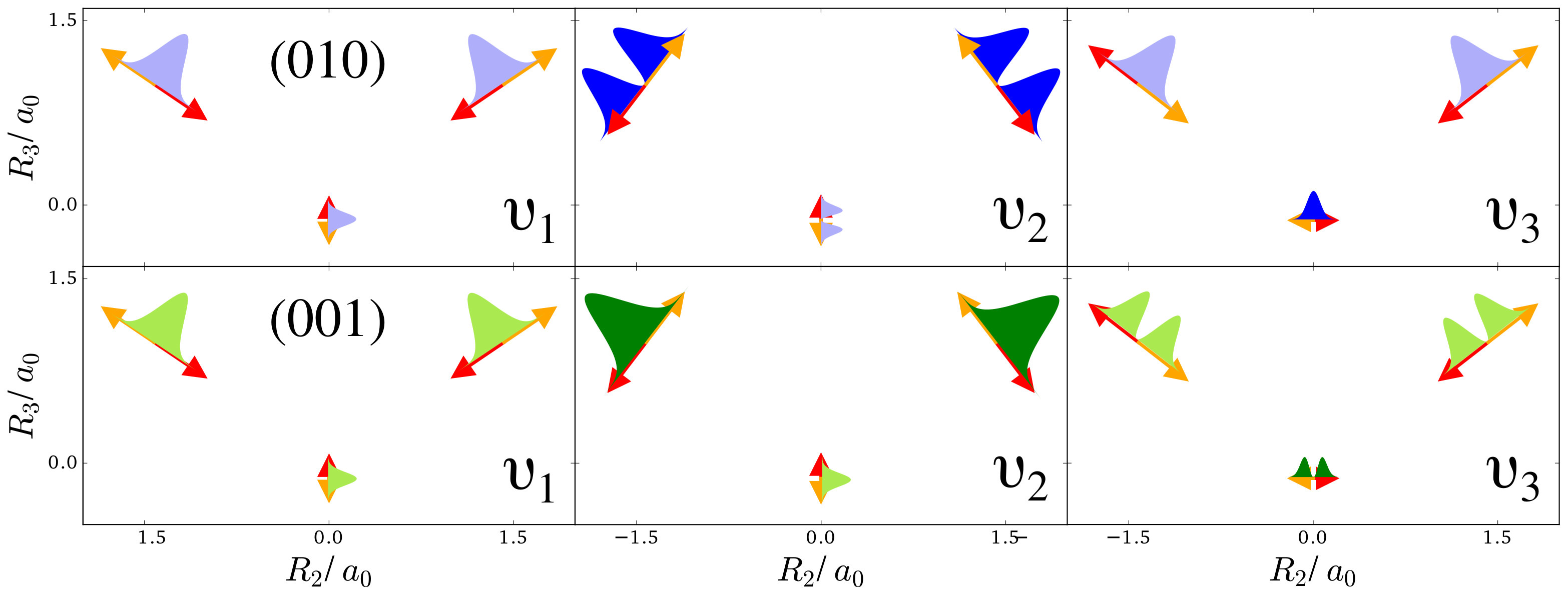 Figure 4
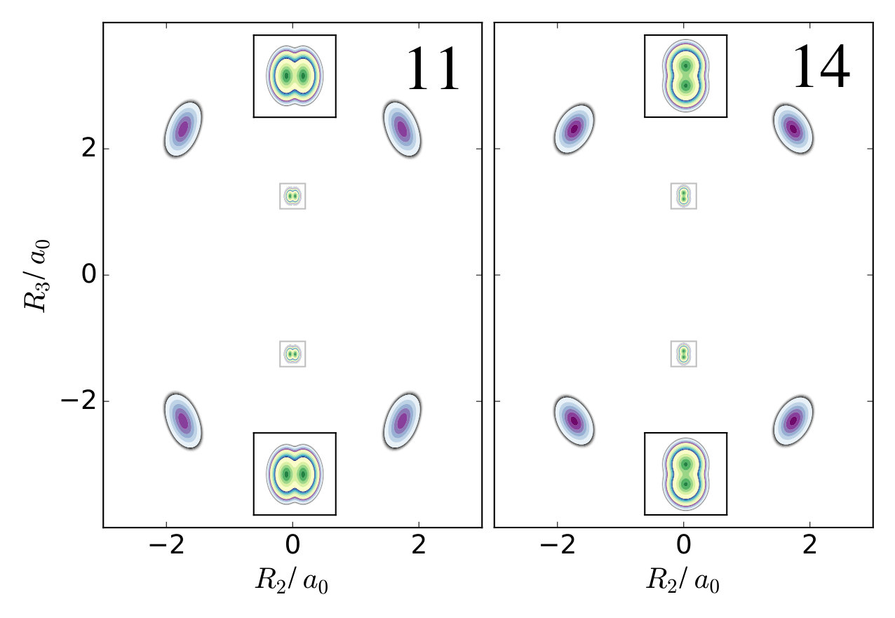 Figure 5
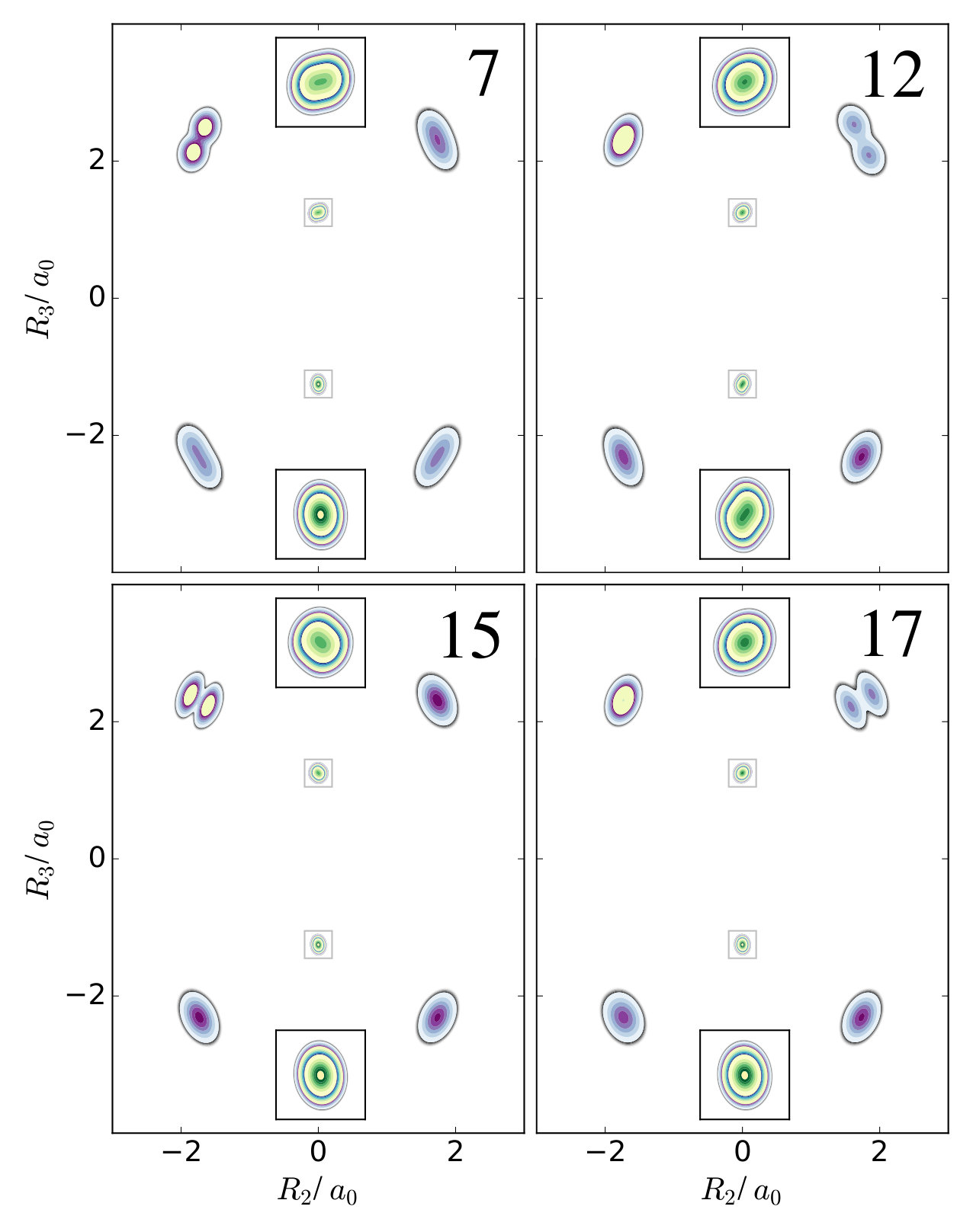 Figure 6
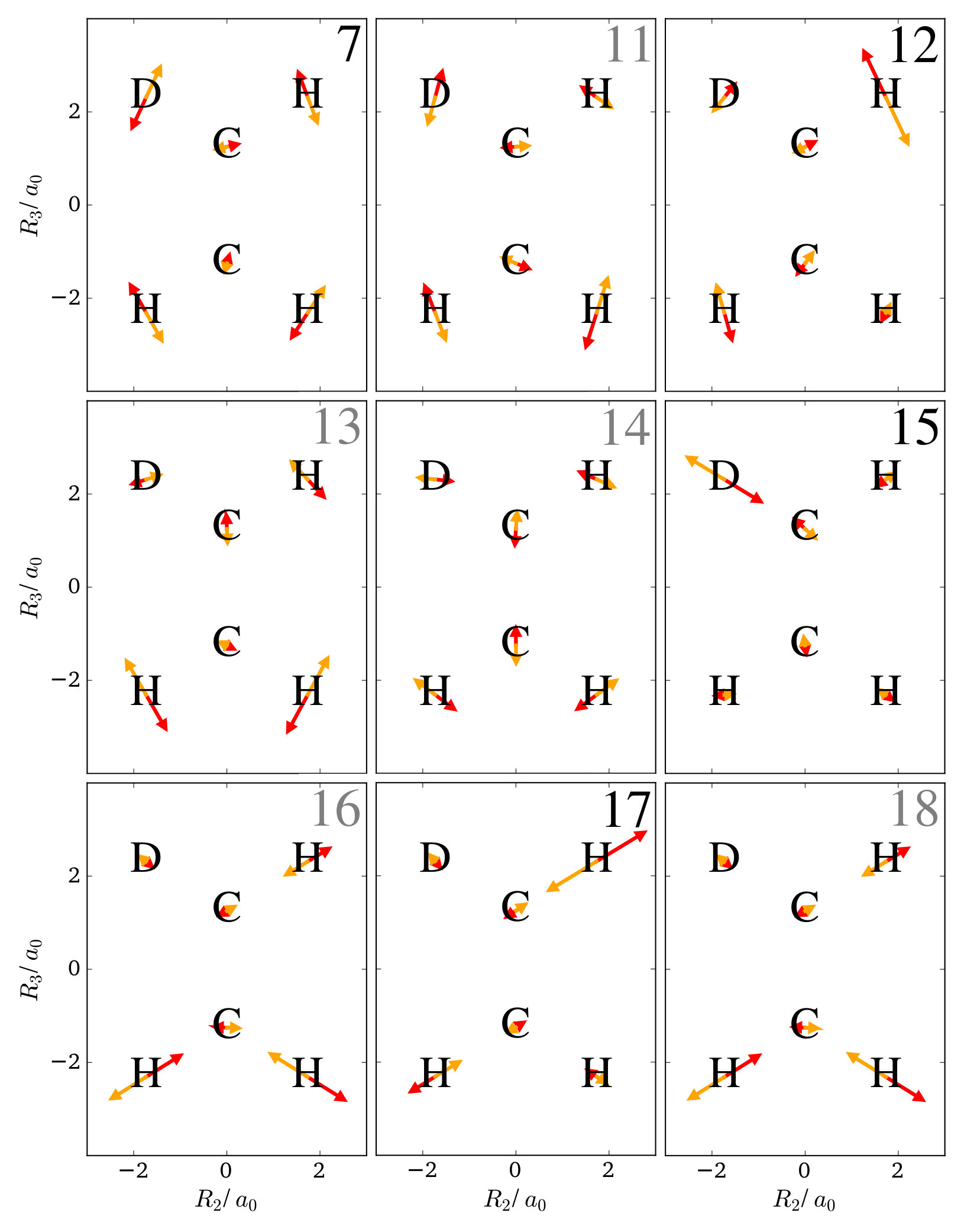 Figure 7
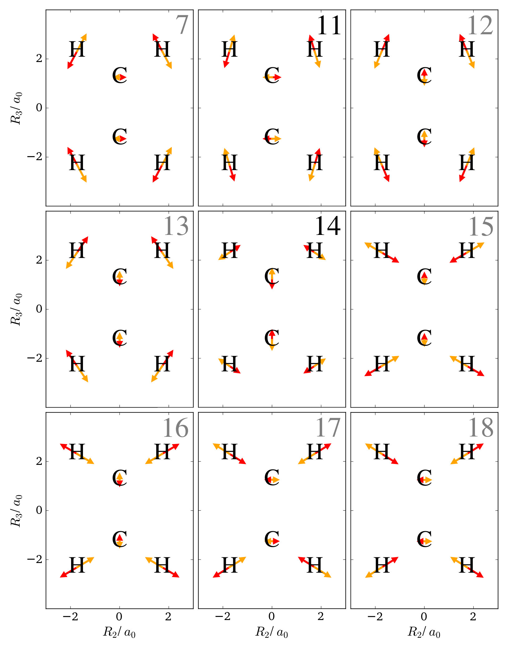 Figure 8
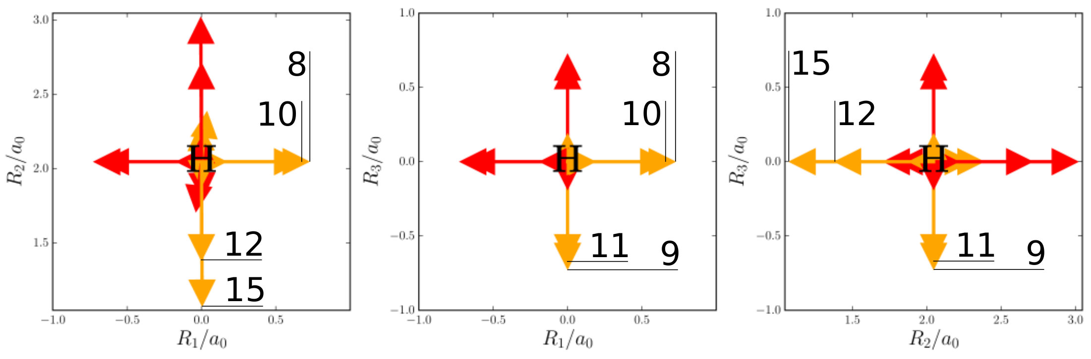 Figure 9
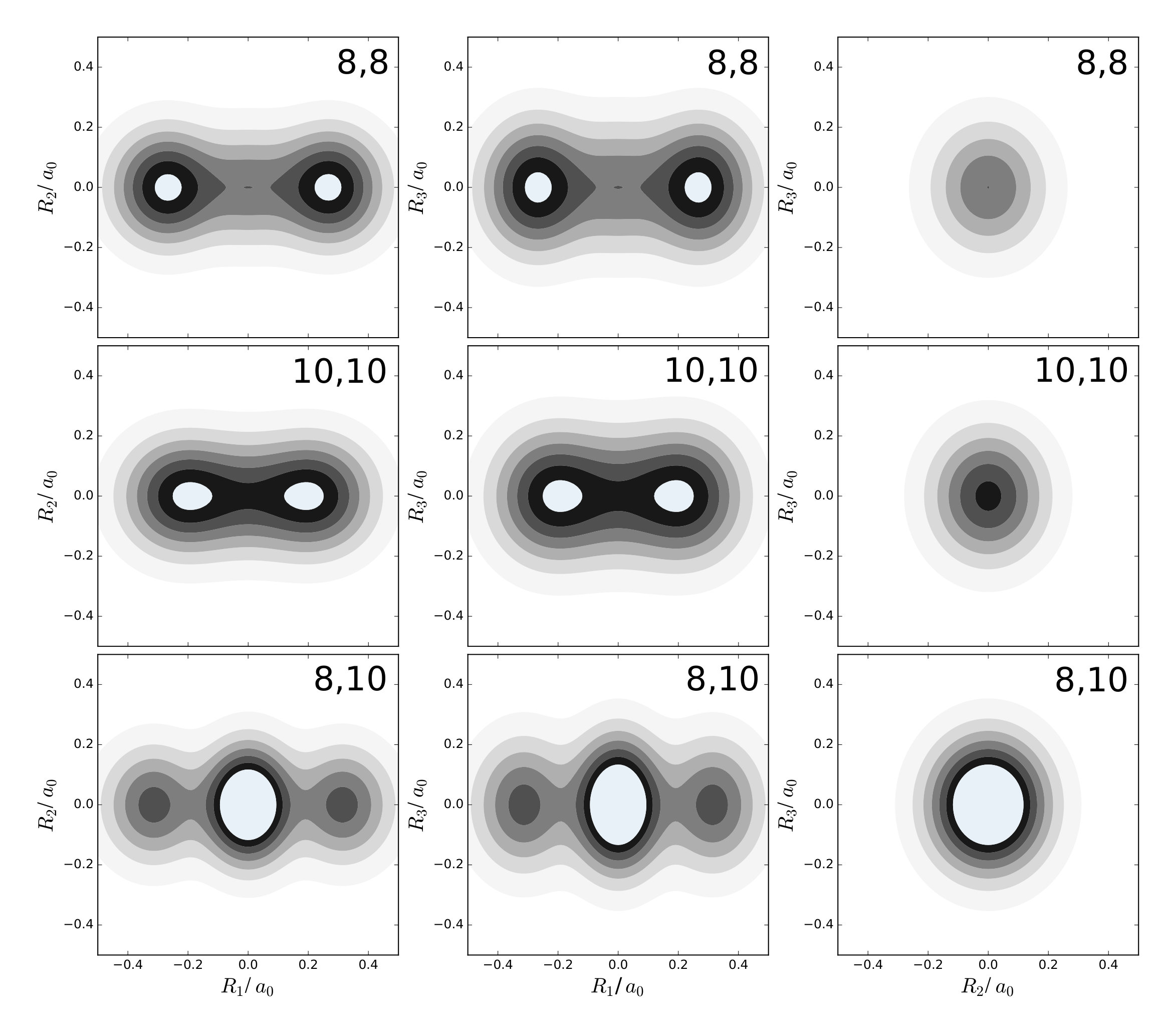 Figure 10
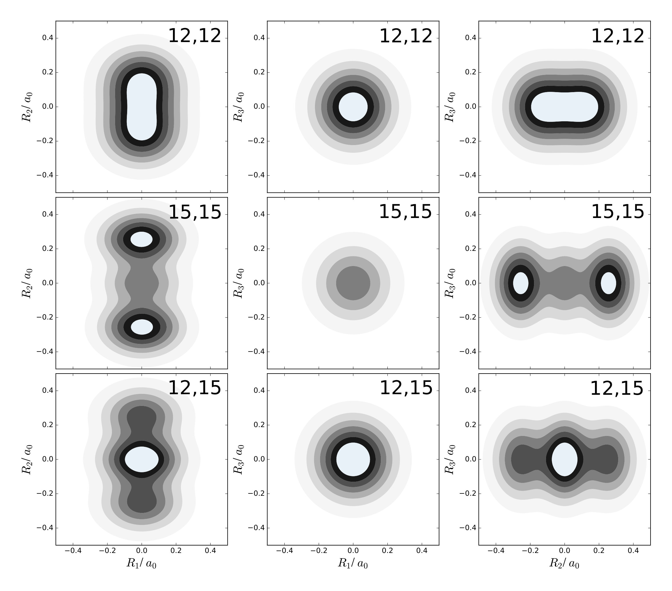 Figure 11
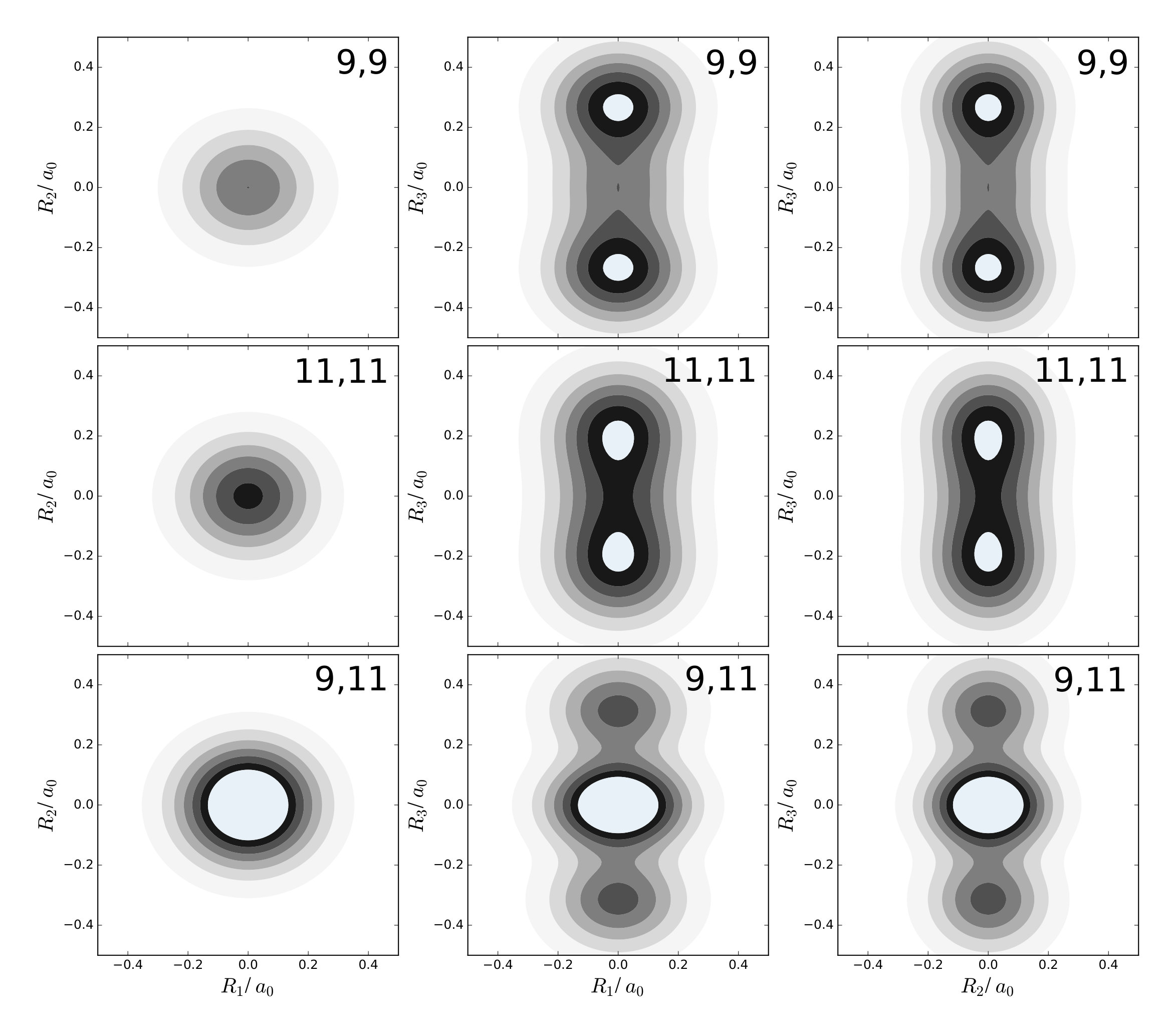 Figure 12
Peer Reviews
No public reviews on file for this paper yet. If you reviewed it on a platform where reviews are public (OpenReview, ICLR, NeurIPS, ICML), you can paste yours below so the community can read it here.
Videos
No videos yet. Explain this paper in a talk, walkthrough, or lecture? Add one.
On the Probability Density of the Nuclei in a Vibrationally Excited Molecule
Axel Schild, Laboratory for Physical Chemistry, ETH Zürich, Switzerland
Abstract
For localized and oriented vibrationally excited molecules, the one-body probability density of the nuclei (one-nucleus density) is studied. Like the familiar and widely used one-electron density that represents the probability of finding an electron at a given location in space, the one-nucleus density represents the probability of finding a nucleus at a given position in space independent of the location of the other nuclei. In contrast to the full many-dimensional nuclear probability density, the one-nucleus density contains less information and may thus be better accessible by experiment, especially for large molecules. It also provides a quantum-mechanical view of molecular vibrations that can easily be visualized. We study how the nodal structure of the wavefunctions of vibrationally excited states translates to the one-nucleus density. It is found that nodes are not necessarily visible: Already for relatively small molecules, only certain vibrational excitations change the one-nucleus density qualitatively compared to the ground state. It turns out that there are some simple rules for predicting the shape of the one-nucleus density from the normal mode coordinates, and thus for predicting if a vibrational excitation is visible in a corresponding experiment.
Quantum-mechanically, the state of an approximately isolated molecule is described by a wavefunction that depends on the location of all nuclei and electrons. The corresponding probability density, which represents the distribution of the particles in the high-dimensional configuration space of their coordinates, is thus difficult to visualize, to comprehend, and also to measure. Notwithstanding, there is an intuitive semi-classical picture of a molecule in chemistry. The emergence of this picture is a non-trivial problem[1, 2] and looking at static states[3, 4, 5] as well as the quantum dynamics[6, 7, 8, 9] of small isolated molecules can lead to surprising insights. An important role for understanding the chemical picture of a molecule is certainly played by the large difference of electronic and nuclear masses. This mass difference results in a strong spatial localization of the nuclei compared to the electrons, which in turn motivates a separation of the molecular wavefunction into a (marginal) nuclear wavefunction and an electronic wavefunction that conditionally depends on the location of the nuclei. While such a separation is exact[10], its practical application is usually in terms of the Born-Oppenheimer approximation [11] where the effect of the nuclear motion on the electronic wavefunction is neglected and only the chosen position of the nuclei is relevant [12].
In the semi-classical picture of a molecule, the theoretical treatment of nuclei and electrons is different: The delocalized electrons are considered to be quantum particles, while the comparably localized nuclei are often approximated as classical particles. However, nuclei are also quantum particles and for small molecules the nuclear (many-body) probability densities have often been calculated and analyzed.[13, 14, 15, 16] Also, there has been recent interest in measuring e.g. the nuclear probability density [17, 18, 19, 20, 21, 22, 23] or the nuclear flux (current) density.[24, 25, 26] An intriguing example of the quantum nature of the nuclei is the measurement of the nuclear density of a vibrationally excited H-molecules by means of Coulomb explosion imaging.[21] The measured nuclear density, which depends only on the relative distance of the two nuclei, shows the expected nodal pattern of vibrationally excited states.
Similar measurements can be made for the electronic probability density, as exemplified by the measurement of the correlated two-electron probability density of the H molecule.[27] For more than two electrons, however, there is a dimensionality problem because multiple electrons have to be measured in coincidence and their probability density is difficult to grasp for the human intuition which is based on a three-dimensional experience of the world. What can be done instead is to consider the electronic one-body probability density, also known as the one-electron density. The one-electron density is the marginal density of finding one electron at a given location in space independent of where the other electrons are. It is the central quantity of Density Functional Theory [28], it is easily visualized, and it is directly accessible to experiment if the molecule is localized: For example, an electron scanning tunneling microscope does essentially measure the one-electron density of a localized molecule and can provide intuitive images of molecules on surfaces [29]. However, while some information about the electronic state can be extracted from the one-electron density,[30] this task is in general difficult: Although the many-electron density is qualitatively different for different excited states due to the appearance of nodes in the wavefunction, the corresponding one-electron densities may be very similar.
Inspired by the experimental imaging of the one-electron density, the question arises if one-nucleus densities can be measured and what information about the nuclear state they contain. To measure a one-nucleus density, only the position of one nucleus relative to the lab frame needs to be measured, hence visualization and interpretation of experimental data can be more direct than in coincidence measurements of the relative position of multiple nuclei. Similar to the one-electron density, the one-nucleus density can also represent a three-dimensional picture of all nuclei if the experiment is insensitive to the type of the nuclei or if the data of different types of nuclei are combined. It can provide a straightforward visualization of the quantum state of the nuclei in a molecule and can in this way complement our understanding of molecular behavior. However, to obtain the one-nucleus density the molecule needs to be localized, e.g. on a surface or with the help of a trap[31]. This author is not aware of any experiments that provide the one-nucleus density of a molecular system with an accuracy that can e.g. resolve vibrational excitations, but in principle such experiments are possible.
Clearly, a measurement of the one-nucleus density would provide a picture of the quantum nature of nuclei that is directly accessible to our spatial conception. But would it provide information about the vibrational state of the molecule, i.e., would the nodal structure of wavefunctions in excited states be visible in the one-nucleus density? This question is investigated in the following with the help of the nuclear wavefunction obtained from a normal mode analysis, i.e., obtained from the local harmonic approximation of the potential energy surface for the nuclear configuration of lowest energy[32]. The nuclear wavefunction is then a product of a translational, a rotational, and a vibrational part,
[TABLE]
The translational part represents translation of the whole molecule in space and can always be factored exactly, while the separation of (which describes rotations of the whole molecule) from is only valid for small displacements from the equilibrium configuration[33, 34, 35, 36]. Typically, a normal mode analysis aims at computing the vibrational frequencies (and maybe analyzing the normal mode coordinates) while is of little interest. However, if those frequencies are in good agreement with measured frequencies, the function is likely also a good approximation to the exact nuclear wavefunction. Then, statements about how qualitative features of translate to the approximate one-nucleus density can be expected to be also true for the exact one-nucleus density.
In the following, the one-nucleus density of the nuclei for different states of is studied and it is investigated how the nodes of the wavefunction in excited states manifest in the one-nucleus density. As shown below, the nuclei are rather localized. In analogy to the classical representation of the nuclei as points in a three-dimensional space, the sum of the one-nucleus densities for all individual (types of) nuclei yields a density in three-dimensional space where the probability distribution of each nucleus is clearly visible. For brevity, hereafter this sum is simply called the one-nucleus density (in analogy to the one-electron density) and the nuclear many-body probability density in the -dimensional configuration space is called the -nucleus density. A detailed description of how the one-nucleus densities are obtained is given in the Supporting Information. Here, only the approximations and assumptions are discussed to point out when the approach is applicable. The aim is to determine the one-nucleus density from the approximate nuclear wavefunction , where is a three-component vector and where stands for the three-component position vectors of the nuclei. The one-nucleus densities for each nucleus are obtained by integrating the -nucleus density over all but the coordinates of the selected nucleus,
[TABLE]
for . The one-nucleus density of the molecule is the sum of the one-nucleus densities for all nuclei,
[TABLE]
The one-nucleus density gives the probability to find any nucleus in a given region of space, but from the relative spatial location it is immediately clear if the nucleus is e.g. an oxygen or a hydrogen nucleus.
The nuclear wavefunction is obtained as follows:
- The Born-Oppenheimer approximation is made to obtain a Schrödinger equation for the nuclear wavefunction alone, with a potential energy surface . Only the electronic ground state is considered.
- A standard normal mode analysis[32] at one of the minima of is made. From this calculation normal mode coordinates and the frequencies of their harmonic oscillator (HO) potentials are obtained. The nuclear wavefunction is a product of HO wavefunctions in each normal mode coordinate, and coupling of rotational and vibrational degrees of freedom is neglected.[34, 35]
- There are six (five for linear molecules) normal modes for which the corresponding HO frequency is zero, representing translation and rotation of the molecule. The nuclear wavefunction has the form of (1). It is assumed that and are normalized Gaussian functions with a very small width corresponding to a frequency of 0.5 . This acts like a constraint on the coordinates and has the effect of localizing and orienting the molecule. The resulting probability density can be interpreted either as a cut through the full density or as the nuclear density given the molecule is at a certain position and oriented in a certain way. A practical advantage of this choice for and is that the wavefunction becomes a product of HO eigenfunctions in all modes. The nuclear wavefunction is
[TABLE]
where is a HO wavefunction with quantum number , and where for the normal mode coordinates for translation and rotation of the whole molecule. In the Supporting Information, it is described how the high-dimensional integral of (2) with wavefunction (4) can be done analytically. All quantum chemical calculations are made with the program Psi4[37] using 3rd order Møller-Plesset pertubation theory and a cc-pVTZ basis set[38].
The first example is the one-nucleus density of the water molecule. Figure 1 shows its familiar vibrations as arrows indicating the motion of classical nuclei. There are three vibrational normal mode coordinates which are labeled according to the usual spectroscopic notation[39]: the symmetric stretch , the bending mode (scissoring) , and the antisymmetric stretch . The one-nucleus densities of the water molecule for some excitations of these modes are shown in Figure 2 as contour plots in the molecular plane, labeled as , where is the quantum number of mode . Insets magnify the details of the nuclear density around the oxygen nucleus, as the density there is much more localized compared to the hydrogen nuclei due to the mass difference.
The one-nucleus density of the vibrational ground state for each nucleus looks like a product of Gaussian functions oriented along the directions of the normal modes (not shown). The one-nucleus densities of the first excitation in each mode, (100), (010), and (001), show how a node in the first excited state of the HO along the corresponding normal modes translates to the one-nucleus density. From the pictures, it seems that the node in the wavefunction of one of these modes leads to a depletion of the one-nucleus density along this normal mode coordinate, but not to exact nodes or nodal planes in the one-nucleus density. There are two reasons for the absence of exact nodes: First, a Gaussian distribution for the translational and rotational modes is assumed. Depending on the width of the these distributions, the resulting one-nucleus densities become broader and loose their structure. A very narrow Gaussian distribution is chosen, hence this reason is of minor importance. The main reasons for the absence of exact nodes in the one-nucleus density is that those nodes only exists in configuration space, while the reduction of the -nucleus density to the one-nucleus density as given in (2) in general does not yield zero anywhere in space.
To understand the one-nucleus density in Figure 2, the analytic form of the -nucleus density needs to be investigated. It is a product of HO densities in all normal modes, because the wavefunction (4) is a product of HO wavefunctions. These 1d-HO densities can be visualized by functions centered at the equilibrium position of the three nuclei, with extent and direction as given by the arrows. In Figure 1, the idea is illustrated for the first excited state of the bending mode, , and of the antisymmetric stretch, .
Some predictions can be made about the qualitative features of the one-nucleus densities at the nuclei by means of a set of simple rules. These rules are called the LOcal COmparison (LOCO) rules, because they are based on a comparison of the normal mode coordinates at the location of each nucleus separately. The LOCO rules are as follows: For a nucleus, the magnitudes and directions of the displacements along the normal modes are compared. (a) If only one normal mode displaces the nucleus in a certain direction or if there is one normal mode that displaces the nucleus in a certain direction much stronger than the other normal modes, the nodes of the wavefunction due to an excitation of this normal mode are clearly visible as depletions in the one-nucleus density. (b) If several normal modes displace the nucleus in the same direction by similar magnitude, an excitation of one of these modes is not necessarily visible in the one-nucleus density. In general, the more such modes exist, the less likely it is that an excitation in one of these can be recognized in the one-nucleus density. It follows that typically, only the normal modes that displace a nucleus the most in a given direction can have a strong influence on the qualitative shape of the one-nucleus density. (c) If there are two (or more) modes that displace the nucleus in the same direction, simultaneous excitation of these modes may show combination features, as exemplified below.
For example, the one-nucleus density of states (100), (010) and (001) can be understood from the LOCO rules (a) and (b) as follows: In Figure 1, sketches of the harmonic oscillator wavefunctions in the modes are shown. At the hydrogen nuclei, and point in a similar direction, while is perpendicular. Thus, the excitation of (state (010)) leads almost to a nodal plane in the one-nucleus density at the hydrogen nuclei, cf. Figure 2. In contrast, excitation of (state (100)) or (state (001)) lead to a significantly less pronounced depletion of the one-nucleus density at the equilibrium position of hydrogen. For the oxygen nucleus, the situation is reversed, as and point in the same direction and is perpendicular. Consequently, the one-nucleus density of state (001) shows a depletion at the oxygen equilibrium position, while no depletion is seen in state (100). As displaces the oxygen nucleus stronger than (which is, however, hardly visible on the scale of Figure 1), a depletion due to the node in is visible in state (010).
A situation similar to that of state (001) is found for states (002) and (003), i.e. when the HO function of is in its second or third excited state. For (002), there is the expected triple-maximum structure at the oxygen nucleus (with a lower central maximum), while the central maximum at the hydrogen nuclei is not visible. For state (003) four maxima are found in the one-nucleus density at the oxygen nucleus (although the two central ones are too weak to be clearly seen in Figure 2), while at the hydrogen nuclei still only two maxima can be found.
An example for LOCO rule (c) is found if two normal modes are excited that locally have similar magnitude and direction. For state (101) three maxima appear at the hydrogen nuclei, similar to a second excited state of the HO, but the central maximum is strongest while the outer maxima are weaker. At the oxygen nucleus only two maxima that point along the direction of normal are found, i.e. a combination of the features of the one-nucleus densities for states (100) (only one maximum in the direction of ) and (001) (two maxima in the direction of ). For states (102) and (201) the qualitative features of the one-nucleus densities can be explained analogously and in accord with the LOCO rules, especially the four maxima at the hydrogen nuclei and a triple maximum at the oxygen nucleus for state (102), but only a double maximum at the state (201).
Last, for state (111) the resulting one-nucleus density is a simple combination of features of states (010) and (101), because is locally perpendicular to the other two vibrational modes at the hydrogen nuclei. At the oxygen nucleus, the effect of exciting two modes with similar direction and magnitude, LOCO rule (c), is that three maxima are found along coordinate upon closer inspection, although the central one is hardly visible.
The normal modes of the water molecule have a symmetry with respect to the hydrogen nuclei. If the symmetry of the nuclear structure is broken by replacing one hydrogen nucleus with a deuterium nucleus, a very different picture for the one-nucleus densities is obtained. The normal mode coordinates for a mono-deuterated water molecule are given in Figure 3. The bending mode is similar to the bending mode of water, but is now the O-D stretch mode that only displaces the deuterium nucleus strongly, while is the O-H stretch mode that almost exclusively displaces the hydrogen nucleus. Thus, according to the LOCO rules it is expected that any excitation of is clearly visible in the one-nucleus density at the hydrogen and deuterium nucleus, that an excitation of is only visible at the deuterium nucleus, and that and excitation of is only visible at the hydrogen nucleus. The prediction of the LOCO rules is accurate, as the one-nucleus densities of the first excited states of each of these modes shown in Figure 3 illustrate.
A consequence of the LOCO rules is that for molecules with many nuclei, only certain (of the lowest) excited states are qualitative visible in the one-nucleus density, i.e. those that are the ones displacing a nucleus the most in a certain direction of space. This is indeed the case. For example, for the benzene molecule the one-nucleus density of none of the first excited states of any normal mode in the molecular plane is qualitatively different from the vibrational ground state. The situation changes if one hydrogen nucleus is exchanged by a deuterium nucleus. In the Supporting Information, the one-nucleus densities for the only two normal mode coordinates that strongly displace the deuterium nucleus are shown. Further examples given in the Supporting Information are an analysis of ethene and mono-deuterated ethene as molecules that contain less nuclei than benzene but where similar effects are found, and methane as an example of a non-planar molecule. The TOC graphic shows the one-nucleus density of one of the vibrational states responsible for the blue color of water.[40]
In conclusion, it is found that similar to how a one-electron density provides understanding of the behavior of electrons, the one-nucleus densities of molecules can provide an interesting opportunity to measure and to visualize the quantum nature of the nuclei: Compared to the -nucleus density, where the location of all nuclei of a molecule needs to be known, the one-nucleus density provides an accessible representation of the nuclear structure that complements the classical picture of the nuclei. While a measurement of the one-nucleus density is undoubtedly difficult because the nuclei are localized in a relatively small region, it is in principle possible, especially for light “quantum” nuclei like hydrogen or deuterium that are comparably delocalized.
Importantly, in contrast to the one-electron density where the electronic state is in general not qualitatively visible (or where, to this authors knowledge, there are no rules available to predict if this is the case), the vibrational state of a molecule may be directly visible in the one-nucleus density. The presented LOCO rules allow to predict, from a normal mode analysis of the nuclear wavefunction, without much effort which vibrational excitations would be visible in the one-nucleus density and thus which molecules are rewarding targets for experimental investigations.
Acknowledgement
The author is grateful to J. Manz (Freie Universität Berlin) for stimulating and supporting this work and to E.K.U. Gross (MPI Halle) for extensive discussions about the topic.
Supporting Information Available: Details of the computation and further examples of one-nucleus densities.
Supporting Information for “On the Probability Density of the Nuclei in a Vibrationally Excited Molecule”: Computational Details
1 The local harmonic approximation
The local harmonic approximation is briefly reviewed. For a detailed description, see [32]. In the Born-Oppenheimer approximation, the nuclear wavefunction is obtained from
[TABLE]
with masses for the coordinates . Around a minimum of , the potential is expanded in a Taylor series to second order in terms of the displacement coordinates and is set to zero. Additionally, mass-weighted displacement coordinates are introduced. Then (5) becomes
[TABLE]
with
[TABLE]
The matrix is diagonalized by the matrix of eigenvectors ,
[TABLE]
where and is the diagonal matrix of the eigenvalues . This yields
[TABLE]
with normal mode coordinates
[TABLE]
In terms of the normal mode coordinates, (5) becomes
[TABLE]
With the coordinate scaling
[TABLE]
the wavefunction becomes a product
[TABLE]
with the eigenfunctions of the quantum harmonic oscillator with unit mass and unit frequency[41, 42]
[TABLE]
where the floor function gives the largest integer smaller than or equal to . However, there is one catch: Six (or five, for linear molecules) of the frequencies are zero, as they belong to translations and rotations of the full system. There are no external potentials that break the translational and rotational invariance of the nuclear system, hence it is broken artificially by setting a non-zero value for these frequencies . The quantum numbers for these degrees of freedom are set to zero so that the density in these modes is a Gaussian function with a width determined by the chosen frequency. In the limit , a -distribution is obtained for .
2 The density
In the main article, the nuclear one-nucleus density is denoted as and it is defined as sum of the individual one-nucleus densities . In this notes it is described how to obtain , but the notation is slightly different. We start from the density in the -dimensional configuration space in terms of displacement coordinates , and we aim at computing the one-nucleus density of the particle with displacement coordinates , by integrating over . To obtain , all we need to do is to shift to the equilibrium position of the considered nucleus, to repeat the procedure for the coordinates of all other nuclei, and to add all those densities. We use the notation because we give the solution of the integrals iteratively, by computing , , etc., with each of the densities in this series depending on one coordinate less compared to the previous density.
The explicit expression for the -body or -coordinate density can now be given. We require that
[TABLE]
and have
[TABLE]
where represents the definite integral throughout this text. Thus, the density is
[TABLE]
with the Jacobian determinant for the coordinate transformation (12) from to that ensures that is normalized to one when integrating over all . Explicitly, with the transformation matrix
[TABLE]
we have
[TABLE]
Then
[TABLE]
with the Gaussian function*** A factor could be added to have properly normalized. Instead, it is included in the definition of the polynomial coefficients.
[TABLE]
and with the polynomial of order
[TABLE]
Before inserting the explicit definition of , we rewrite this polynomial by changing the summation variables to , , so that
[TABLE]
with coefficients
[TABLE]
that are obtained with summation boundaries
[TABLE]
An alternative that is more practical for numerical implementations is to change the summation variables to , , so that the coefficients become
(27)
(28)
where the sum over now has increments .
3 Initial parameters
The general form of the -nucleus density (21) is
[TABLE]
with the Gaussian function (22) given as
[TABLE]
It is a multivariate Gaussian function multiplied by a polynomial composed of monomials of degree , where
[TABLE]
is the sum of quantum numbers. The superscript of the coefficients for the monomials and indicates that those are the parameters of the -nucleus density. Below, we see that when we integrate over coordinate we obtain an -nucleus density that looks like (29), except that the sums terminate at and the coefficients changed. By determining the new coefficients, we can perform all integrals that are necessary to derive the one-nucleus density iteratively. Note that the Jacobian determinant is included in the initial coefficients, cf. (36).
However, first we have to determine the initial values of the coefficients. Inserting the transformation equation of the coordinates (12),(18) into the definition of the Gaussian function (22) yields
[TABLE]
Similarly, inserting (12),(18) into the definition of the polynomials (24) for each quantum number shows that these polynomials are a sum (over ) of monomials
[TABLE]
with coefficients†††These coefficients are symmetric w.r.t. exchange of any two indices.
[TABLE]
The polynomial occurring in the definition of the density (21) is
[TABLE]
By comparing the definition of the coefficients in the density (29) with the from of the polynomial (35) we see how to obtain the coefficients : First, we compute all monomial coefficients (34). Then, we take the tensor product along ,‡‡‡These coefficients are not symmetric w.r.t. exchange of any two indices anymore, but only within certain blocks. This makes the equations later a little bit more elaborate.
[TABLE]
for all possible combinations of the -index. The number of indices of the resulting object is the sum of the number of indices of the individual coefficients and corresponds to the order of the polynomial to which it belongs. Adding all the results of the same order yields the initial coefficients of the -nucleus density.
4 Integration
Next, we need to integrate over one variable, say, . For this purpose, we need the integral§§§ is still the definite integral from to . [42]
[TABLE]
Taking the derivative of (37) w.r.t. and comparing with the definition of the Hermite polynomials yields
[TABLE]
Integrating the density (29) over yields
[TABLE]
Here, represents the coefficient for the monomial of order with indices that run from to , and the remaining indices set to . The operator constructs the sum of all permutations of the indices set to with those that run from to .
To perform the integral of the density over the last coordinate , we first have to group the monomials in (29) for each order according to the exponent of (which corresponds to the index of ) to find
(40)
At each order , the coefficients of each integral are obtained as sum of the possible permutations of the index occurring times in the coefficients . Unfortunately, in general is not symmetric when exchanging two indices. However, it is constructed as tensor product of arrays that have this property, hence this symmetry may be exploited to some extent, if desired.
We now assume (correctly) that has the same functional form as , but with new coefficients and ,
[TABLE]
The integrals that occur here are of the form (38) and are given by
[TABLE]
and
[TABLE]
respectively.
Equations (42) and (43) can be derived from (37) and (38) by making the identifications
(44)
We see from (42) that because occurs in all integrals , the new coefficients for the exponential are
[TABLE]
The new coefficients for the polynomial are
[TABLE]
Some remarks are in order: First, we note that the indices now only have entries. Second, the term of the last equation has to be read as follows: We take and set the last indices equal to . Then, we make a tensor multiplication with so many vectors that the resulting object has indices.
The second step of the integration of over is to group the resulting polynomial according to the orders of the monomials and add the respective contributions. The structure of can be visualized as follows:
\mathtt{}\displaystyle\binom{0}{0}[0]\oplus[{\color[rgb]{0.8,0.4,0.0}0_{0}}]
(i=0)
\mathtt{}\displaystyle\binom{2}{0}[2]\oplus[{\color[rgb]{0.9,0.6,0.0}0_{0}}]+\binom{2}{1}[1]\oplus[{\color[rgb]{0.9,0.6,0.0}1_{0}}]+\binom{2}{2}[0]\oplus[{\color[rgb]{0.8,0.4,0.0}0_{1}},{\color[rgb]{0.9,0.6,0.0}2_{0}}]
(i=1)
\mathtt{}\displaystyle\binom{4}{0}[4]\oplus[{\color[rgb]{0.0,0.6,0.5}0_{0}}]+\binom{4}{1}[3]\oplus[{\color[rgb]{0.0,0.6,0.5}1_{0}}]+\binom{4}{2}[2]\oplus[{\color[rgb]{0.9,0.6,0.0}0_{1}},{\color[rgb]{0.0,0.6,0.5}2_{0}}]+\binom{4}{3}[1]\oplus[{\color[rgb]{0.9,0.6,0.0}1_{1}},{\color[rgb]{0.0,0.6,0.5}3_{0}}]+\binom{4}{4}[0]\oplus[{\color[rgb]{0.8,0.4,0.0}0_{2}},{\color[rgb]{0.9,0.6,0.0}2_{1}},{\color[rgb]{0.0,0.6,0.5}4_{0}}]
(i=2)
\mathtt{}\displaystyle\binom{6}{0}[6]\oplus[{\color[rgb]{0.8,0.6,0.7}0_{0}}]+\binom{6}{1}[5]\oplus[{\color[rgb]{0.8,0.6,0.7}1_{0}}]+\binom{6}{2}[4]\oplus[{\color[rgb]{0.0,0.6,0.5}0_{1}},{\color[rgb]{0.8,0.6,0.7}2_{0}}]+\binom{6}{3}[3]\oplus[{\color[rgb]{0.0,0.6,0.5}1_{1}},{\color[rgb]{0.8,0.6,0.7}3_{0}}]+\binom{6}{4}[2]\oplus[{\color[rgb]{0.9,0.6,0.0}2_{2}},{\color[rgb]{0.0,0.6,0.5}3_{1}},{\color[rgb]{0.8,0.6,0.7}4_{0}}]+\binom{6}{5}[1]\oplus[{\color[rgb]{0.9,0.6,0.0}1_{2}},{\color[rgb]{0.0,0.6,0.5}3_{1}},{\color[rgb]{0.8,0.6,0.7}5_{0}}]+\binom{6}{6}[0]\oplus[{\color[rgb]{0.8,0.4,0.0}0_{3}},{\color[rgb]{0.9,0.6,0.0}2_{2}},{\color[rgb]{0.0,0.6,0.5}4_{1}},{\color[rgb]{0.8,0.6,0.7}6_{0}}]
(i=3)
The binomial coefficients are a reminder of the permutations induced by the permutation operator acting on . The number left of is the degree of the polynomial that is not included in the integration (as it does not contain the integration variable), and has the coefficient . The numbers are the degrees of the polynomials coming from the integral . The means that the orders have to be added, i.e. represents one monomial of order and one monomial of order in the final expression. The colors of the numbers right of indicate the same order of the resulting monomial and the subscript indicates the number of (43) from which the monomial is obtained. We note that all contributions to come from the terms for , all contributions to come from the terms for , etc. From this structure, (46) can be obtained as follows: First, we change the labels of the summation variables of the coordinates in (43) from to ,
(47)
so that we can insert this formula directly into the equation for the density after first integration (39),
(48)
(49)
Now we have to identify of (49) in (48) by setting and by ensuring that the limits of the sums over and are adjusted accordingly.
To obtain the one-nucleus density, equations (45) and (46) need to be iterated until only three indices are left. Those belong to the displacement coordinates . In order to obtain the one-nucleus density for the other nuclei, the procedure is repeated after appropriate permutation of the columns of transformation matrix .
Last, we note that that we could ignore all factors in the original and updated coefficients because each integration cancels one of the of the initially factors. Then we need to multiply the final one-nucleus density with to obey the normalization condition.
5 Note on the computational implementation
The approximations that are used for the nuclear wavefunction allow to compute the vibrational one-nucleus densities for molecules with a relatively large number of nuclei . However, the resulting polynomial is of order , where is the sum of the vibrational quanta in the system. The current numerical implementation stores arrays of the polynomial coefficients that are of dimension , hence with the number of quanta the memory limit is quickly reached, so that in practice only computations for are possible on a modern workstation. With a different numerical implementation this problem can possibly be avoided, but for large the local harmonic approximation that is made in the normal mode analysis is questionable anyway, hence this is not practical restriction.
Supporting Information for “On the Probability Density of the Nuclei in a Vibrationally Excited Molecule”: Additional Examples
A note on the labeling of the normal modes: * In contrast to the main article, molecules with more that three nuclei are discussed in the following, hence there are more normal modes. To have a uniform and simple notation for all molecules, the following convention is used to label the normal modes: The normal modes are numbered according to the frequency of their corresponding harmonic oscillators in ascending order. Modes 1 to 6 are those of translation and rotation of the molecule. The symmetry of the mode is ignored in the numbering. *
A note on the labeling of the states: * In these document, only one-nucleus densities for a single excitation of one mode or, for methane, for two singly excited modes or one double excited mode are shown. The state is labeled by the number(s) of the excited modes. *
In the following, present one-nucleus densities for selected states of water, mono-deterated benzene, ethene, mono-deuterated ethene (D-ethene), and methane are presented and it is discussed how their qualitative shape can be predicted by using the LOCO rules and the normal mode coordinates. All computations were performed as described in the main article, hence the Born-Oppenheimer approximation is used in a local harmonic approximation at the nuclear configuration of minimum energy (the equilibrium configuration), and it is assumed that the molecule is localized and oriented. The three-dimensional reference space has coordinates . For each molecule, first the normal mode coordinates are discussed and thereafter selected densities are presented.
As mentioned in the main article, for the benzene molecule the first excitations of any of the normal mode coordinates do not lead to a qualitative change of the one-nucleus density compared to the ground state because the hydrogen and oxygen nuclei are displaced in the same direction by multiple normal modes. In contrast, for mono-deterated benzene there are only two normal modes that significantly displaced the deuterium nucleus. These coordinates are also perpendicular with respect to each other, hence their excitations are clearly visible in the one-nucleus density. This is shown in figure 4.
The equilibrium configuration of ethene is planar, hence the normal mode coordinates correspond to displacements of the nuclei that are either completely in the molecular plane, or perpendicular. Hence, the discussion is restricted to the normal modes in the molecular plane, which is defined as the - plane. For ethene, figure 5 shows the selected normal mode coordinates. The modes are numbered by increasing frequency of the corresponding harmonic oscillator, and modes 1-6 are those of translation and rotation of the whole system.
From the figure, it can be seen that at the hydrogen nuclei there are many normal modes that correspond to displacements in a similar spatial direction, which also have similar magnitude. For example, modes 7, 11, 12, and 13 all displace the hydrogen nuclei to a similar extend in a similar direction, while modes 15, 16, 17, and 18 do the same in an almost perpendicular direction. Hence, from the LOCO rules it can be concluded that an excitation of just one of these modes does not yield any notable qualitative changes of the one-nucleus density, i.e. there are no new clear minima appearing that correspond to the nodes of the wavefunction in such an excited state. This is indeed the case, and all one-nucleus densities for an excitation along one of these modes is qualitatively similar to the ground state.
The situation at the carbon nuclei, however, is somewhat different. Although there are again many modes that displace these nuclei in the same direction, there are two modes that displace them stronger than all other modes: Mode 11 displaces the oxygen nuclei comparably strongly along , while mode 14 displaces the oxygen nuclei comparably strongly along . This difference can be seen in the one-nucleus densities for the respective excited states. Figure 6 shows contour plots of the one-nucleus densities for the first excited states of mode 11 and mode 14, and insets show a magnification of the regions around the carbon nuclei. Several contour maps with different line spacing are used to be able to see details of the density of the hydrogen nuclei and of the carbon nuclei in the same picture. The density at those nuclei has two local maxima and a depletion in the region of the equilibrium position. No other of the excited states corresponding to the first excitation any of the normal modes shows this qualitative features, neither at the carbon nuclei nor at the hydrogen nuclei.
The situation is altered if the symmetry is broken by isotope substitution. The normal mode coordinates for D-ethene are given in figure 7. As is clear from the figure, there are several normal modes that should, if excited, according to the LOCO rules yield a clear qualitative imprint in the one-nucleus density, because they are the only ones that displace the considered nucleus significantly in a certain direction. To illustrate, normal modes 7, 12, 15, and 17 are used. Normal modes 7 and 15 are the ones that displace the deuterium nucleus the strongest, and in almost perpendicular directions. Modes 12 and 17 displace the top-right hydrogen nucleus the strongest, and also in mutually almost perpendicular directions. Consequently, excitations of those modes can be expected to have the strongest qualitative impact on the one-nucleus density at the given nucleus.
Figure 8 shows the one-nucleus density for the excites states represented by first excitation of modes 7, 12, 15, or 17. It can clearly be seen that excitations of mode 7 and 15 as well as 12 and 17 show two maxima and a depletion corresponding to the node in the wavefunction of the excited state, at the deuterium nucleus and the top-right hydrogen nucleus, respectively. There are more examples of this behavior at the other nuclei, but none of these is as pronounced as the ones depicted in figure 8.
Last, it should be illustrated that the LOCO rules also hold for non-planar molecules. For this purpose, methane is considered. In its equilibrium configuration, this molecule has four hydrogen nuclei at the vertices of a tetrahedron, and a carbon nucleus at its center. As it is hard to draw the one-nucleus density of the nuclei in a picture, only one of the four equivalent hydrogen nuclei is considered. For the carbon nucleus being at the origin, this nucleus is located at ca. . All normal mode coordinates at this nucleus are shown in figure 9 as arrows in the --, --, and --plane.
From the figure, it can be seen that at this nucleus, in each direction there are only two relevant normal modes: mode 8 and 10 along , mode 12 and 15 along , and mode 9 and 11 along . Mode 8, 15, and 9 are those displacing the nucleus the strongest, although only mode 15 has a clear margin with respect to mode 12, while the displacement along modes 10 and 11 are very close to those of modes 8 and 9, respectively
In this example, the excited states corresponding to two quanta in these modes are considered. Contour plots of the one-nucleus densities are given in figure 10 for excitations of mode 8 and 10, in figure 11 for excitations of mode 12 and 15, and in figure 12 for excitations of mode 9 and 11.
It is found that a double excitation of mode 15 has a clear triple-maximum structure reminiscent of the density of the harmonic oscillator wavefunction in this node. According to the LOCO rules this is expected, because mode 15 displaces the considered nucleus the most. Also double excitations of modes 8 or 9 yield triple-maximum structures, although the central maximum is almost invisible. Again, this can be rationalized because the wavefunction is in its ground state along modes 10 and 11, which have similar effects on the nucleus.
The combined effect of exciting two locally similar modes can also be observed. In figures 10, 11, and 12, the one-nucleus density of the excited state corresponding to an excitation of mode 8 and 10, mode 12 and 15, and mode 9 and 11 are also shown. A triple-maximum structure is found, which is most pronounced when the two modes are locally similar, i.e. for excitation of mode 8 and 10 as well as mode 9 and 11.
The reference list from the paper itself. Each links out to its DOI / PubMed record.
- 1[1] Brian T. Sutcliffe and R. Guy Woolley. Molecular structure calculations without clamping the nuclei. Phys. Chem. Chem. Phys. , 7(21):3664, 2005.
- 2[2] Brian Sutcliffe. To what question is the clamped-nuclei electronic potential the answer? Theor. Chem. Acc. , 127(3):121, 2010.
- 3[3] Edit Mátyus, Jürg Hutter, Ulrich Müller-Herold, and Markus Reiher. On the emergence of molecular structure. Phys. Rev. A , 83(5):052512, 2011.
- 4[4] Edit Mátyus, Jürg Hutter, Ulrich Müller-Herold, and Markus Reiher. Extracting elements of molecular structure from the all-particle wave function. J. Chem. Phys , 135(20), 2011.
- 5[5] Edit Mátyus and Markus Reiher. Molecular structure calculations: A unified quantum mechanical description of electrons and nuclei using explicitly correlated Gaussian functions and the global vector representation. J. Chem. Phys , 137(2), 2012.
- 6[6] Jörn Manz, Jhon Fredy Pérez-Torres, and Yonggang Yang. Vibrating H 2 + \mathtt{}_{2}^{+} ( 2 Σ g + \mathtt{}^{2}\Sigma_{\rm g}^{+} , J M = 00 𝐽 𝑀 00 \mathtt{}JM=00 ) Ion as a Pulsating Quantum Bubble in the Laboratory Frame. J. Phys. Chem. A , 118:8411, 2014.
- 7[7] Timm Bredtmann, Dennis J. Diestler, Si-Dian Li, Jörn Manz, Jhon Fredy Pérez-Torres, Wen-Juan Tian, Yan-Bo Wu, Yonggang Yang, and Hua-Jin Zhai. Quantum theory of concerted electronic and nuclear fluxes associated with adiabatic intramolecular processes. Phys. Chem. Chem. Phys. , 17:29421–29464, 2015.
- 8[8] Jhon Fredy Pérez-Torres. Dissociating H 2 + \mathtt{}_{2}^{+} ( 2 Σ g + \mathtt{}^{2}\Sigma_{\rm g}^{+} , J M = 00 𝐽 𝑀 00 \mathtt{}JM=00 ) Ion as an Exploding Quantum Bubble. J. Phys. Chem. A , 119:2895, 2015.