Linear Analysis of Fast-Pairwise Collective Neutrino Oscillations in Core-Collapse Supernovae based on the Results of Boltzmann Simulations
Milad Delfan Azari, Shoichi Yamada, Taiki Morinaga, Wakana Iwakami,, Hirotada Okawa, Hiroki Nagakura, Kohsuke Sumiyoshi

TL;DR
This study investigates the potential for fast-pairwise neutrino flavor conversions in core-collapse supernovae using realistic Boltzmann simulation data, finding no signs of conversion in the examined scenarios but exploring conditions for possible conversion.
Contribution
First application of linear analysis to realistic supernova neutrino distributions from Boltzmann simulations to assess flavor conversion potential.
Findings
No positive signs of neutrino flavor conversion in the studied model.
Detailed analysis of conditions required for flavor conversion.
Modified distributions suggest possible conversion under certain conditions.
Abstract
Neutrinos are densely populated deep inside the core of massive stars after their gravitational collapse to produce supernova explosions and form compact stars such as neutron stars (NS) and black holes (BH). It has been considered that they may change their flavor identities through so-called fast-pairwise conversions induced by mutual forward scatterings. If that is really the case, the dynamics of supernova explosion will be influenced, since the conversion may occur near the neutrino sphere, from which neutrinos are effectively emitted. In this paper, we conduct a pilot study of such possibilities based on the results of fully self-consistent, realistic simulations of a core-collapse supernova explosion in two spatial dimensions under axisymmetry. As we solved the Boltzmann equations for neutrino transfer in the simulation not as a post-process but in real time, the angular…
Click any figure to enlarge with its caption.
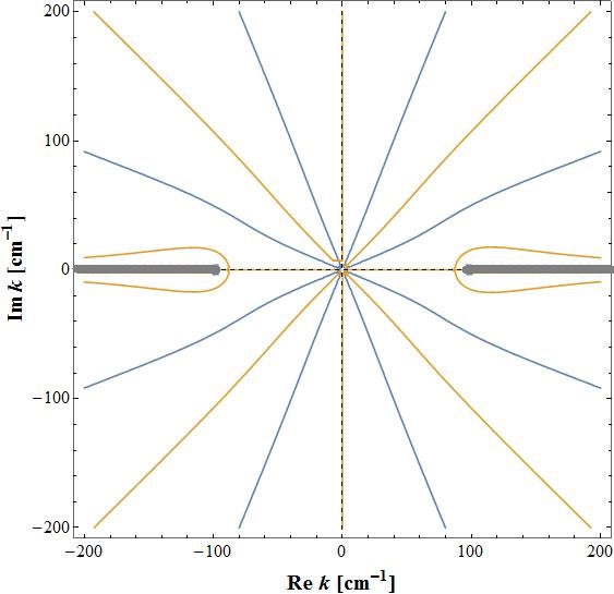 Figure 1
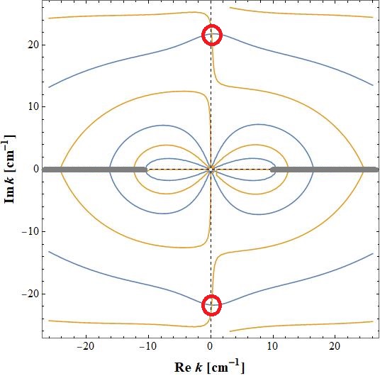 Figure 2
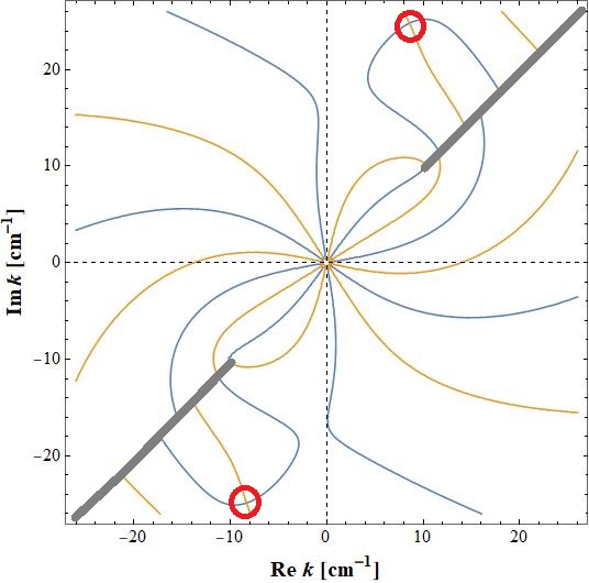 Figure 3
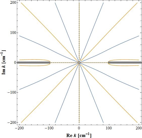 Figure 4
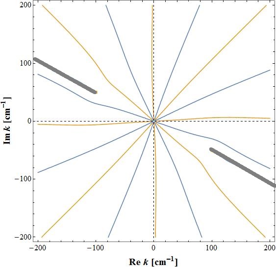 Figure 5
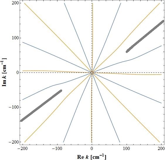 Figure 6
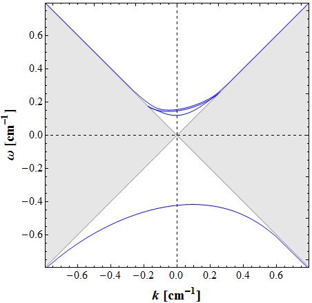 Figure 7
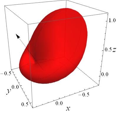 Figure 8
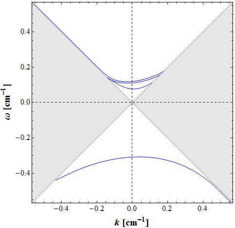 Figure 9
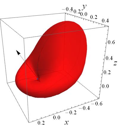 Figure 10
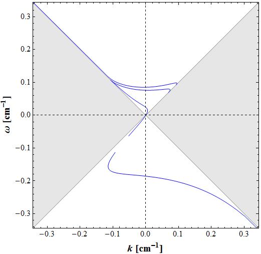 Figure 11
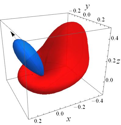 Figure 12
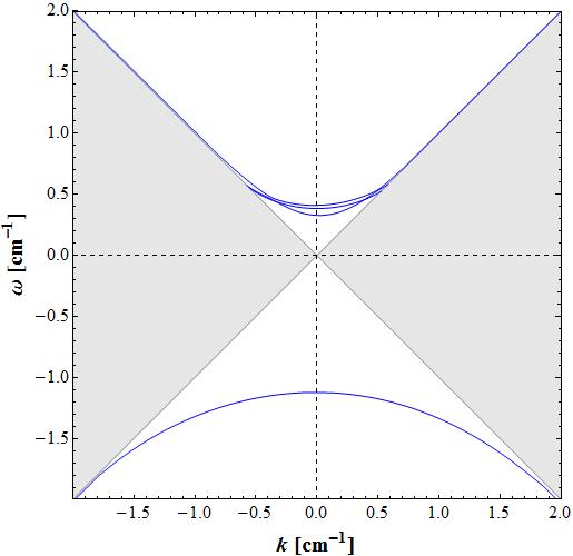 Figure 13
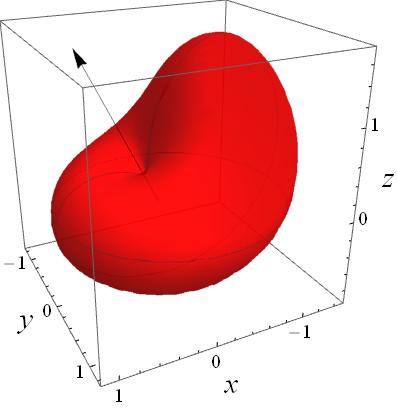 Figure 14
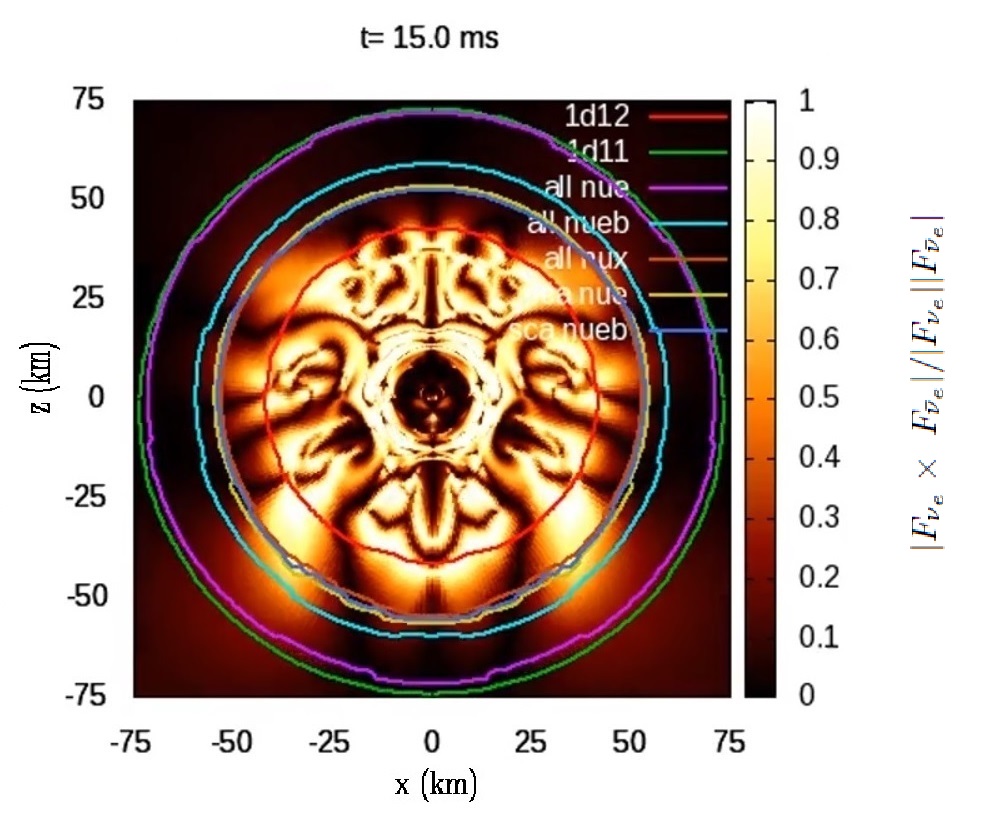 Figure 15
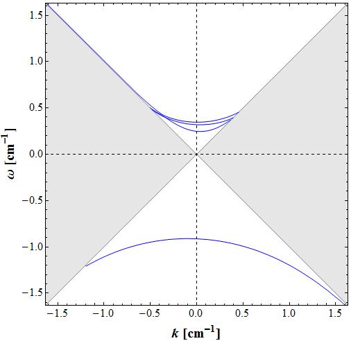 Figure 16
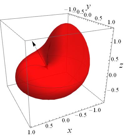 Figure 17
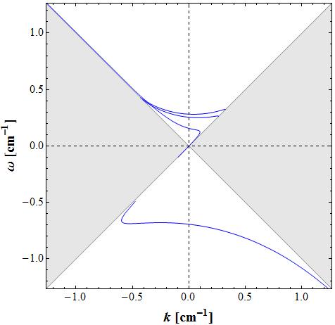 Figure 18
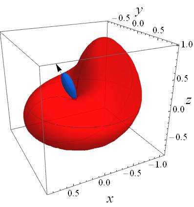 Figure 19
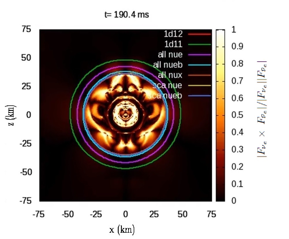 Figure 20
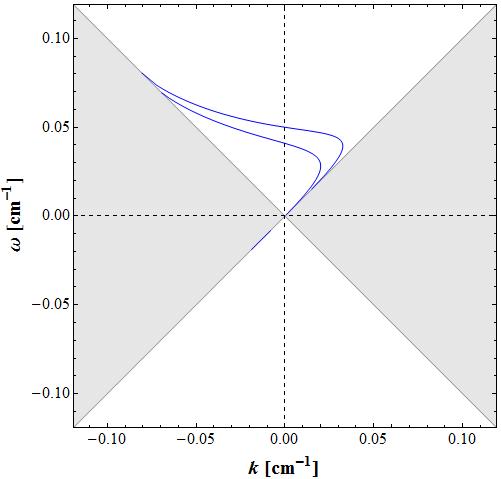 Figure 21
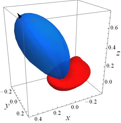 Figure 22
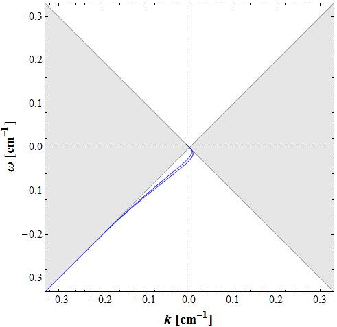 Figure 23
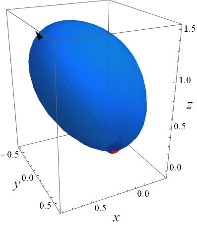 Figure 24
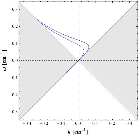 Figure 25
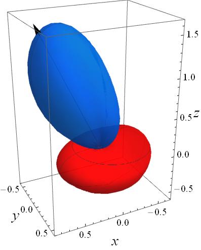 Figure 26
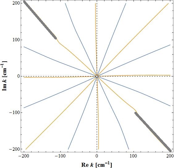 Figure 27
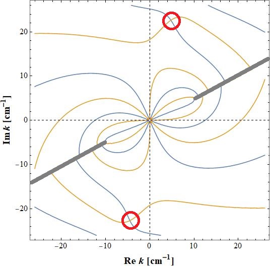 Figure 28
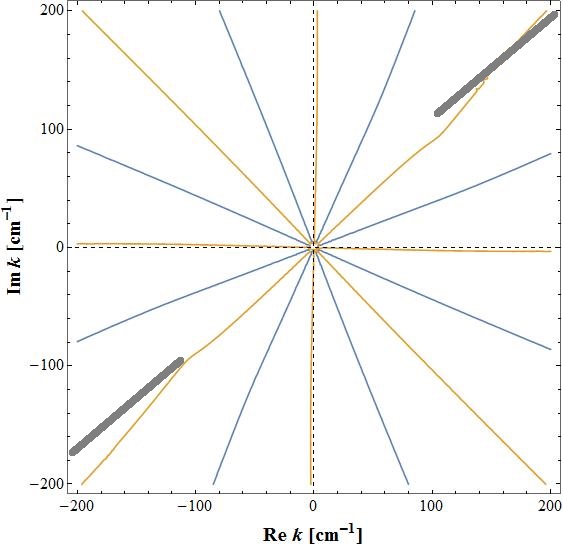 Figure 29
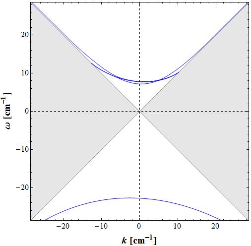 Figure 30
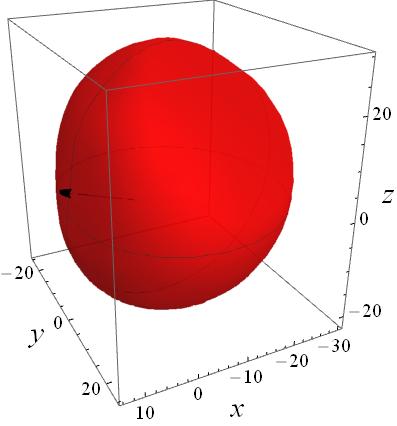 Figure 31
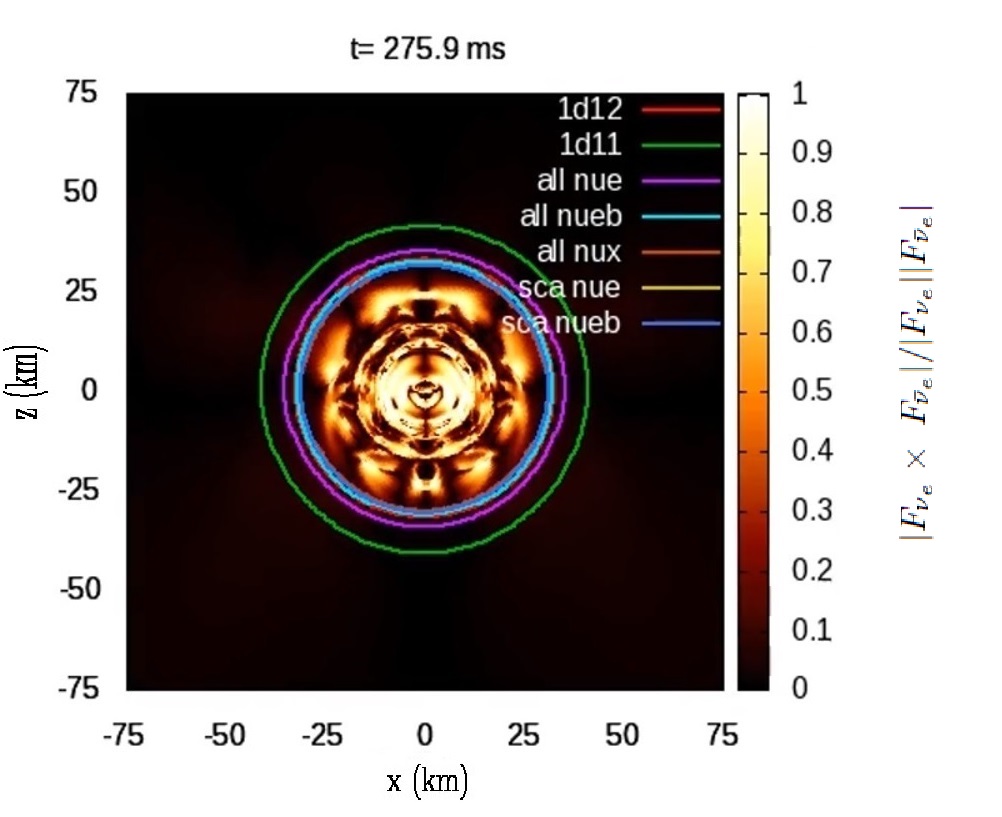 Figure 32
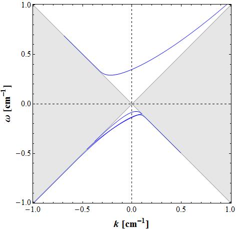 Figure 33
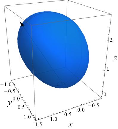 Figure 34
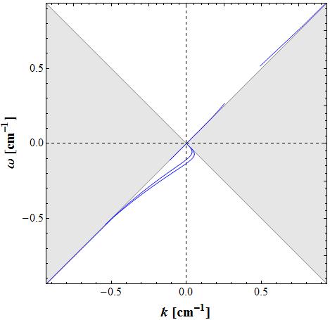 Figure 35
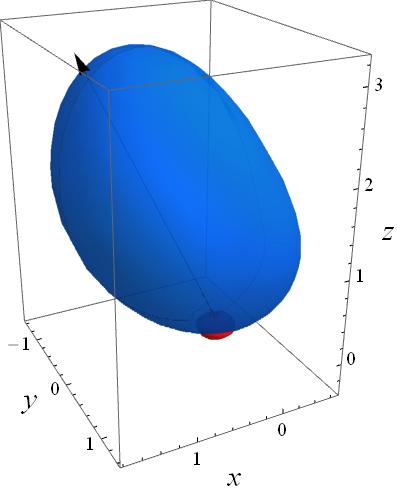 Figure 36
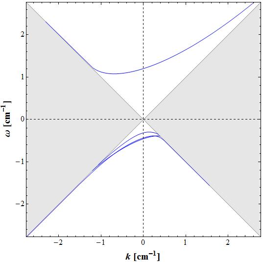 Figure 37
 Figure 38
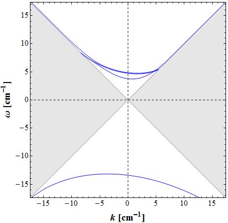 Figure 39
 Figure 40
Peer Reviews
No public reviews on file for this paper yet. If you reviewed it on a platform where reviews are public (OpenReview, ICLR, NeurIPS, ICML), you can paste yours below so the community can read it here.
Videos
No videos yet. Explain this paper in a talk, walkthrough, or lecture? Add one.
Linear Analysis of Fast-Pairwise Collective Neutrino Oscillations in Core-Collapse Supernovae based on the Results of Boltzmann Simulations
Milad Delfan Azari
Department of Physics, Graduate School of Advanced Science and Engineering, Waseda University, 3-4-1 Okubo, Shinjuku, Tokyo 169-8555, Japan
Shoichi Yamada
Department of Physics, Graduate School of Advanced Science and Engineering, Waseda University, 3-4-1 Okubo, Shinjuku, Tokyo 169-8555, Japan
Advanced Research Institute for Science and Engineering, Waseda University, 3-4-1 Okubo, Shinjuku, Tokyo 169-8555, Japan
Taiki Morinaga
Department of Physics, Graduate School of Advanced Science and Engineering, Waseda University, 3-4-1 Okubo, Shinjuku, Tokyo 169-8555, Japan
Wakana Iwakami
Advanced Research Institute for Science and Engineering, Waseda University, 3-4-1 Okubo, Shinjuku, Tokyo 169-8555, Japan
Yukawa Institute for Theoretical Physics, Kyoto University,Oiwake-cho, Kitashirakawa, Sakyo-Ku, Kyoto, 606-8502, Japan
Hirotada Okawa
Advanced Research Institute for Science and Engineering, Waseda University, 3-4-1 Okubo, Shinjuku, Tokyo 169-8555, Japan
Yukawa Institute for Theoretical Physics, Kyoto University,Oiwake-cho, Kitashirakawa, Sakyo-Ku, Kyoto, 606-8502, Japan
Waseda Institute for Advanced Study, 1-6-1 Nishi Waseda, Shinjuku, Tokyo 169-8050, Japan
Hiroki Nagakura
Department of Astrophysical Sciences, Princeton University, Princeton, NJ 08544, USA
Kohsuke Sumiyoshi
Numazu College of Technology, Ooka 3600, Numazu, Shizuoka 410-8501, Japan
Abstract
Neutrinos are densely populated deep inside the core of massive stars after their gravitational collapse to produce supernova explosions and form compact stars such as neutron stars (NS) and black holes (BH). It has been considered that they may change their flavor identities through so-called fast-pairwise conversions induced by mutual forward scatterings. If that is really the case, the dynamics of supernova explosion will be influenced, since the conversion may occur near the neutrino sphere, from which neutrinos are effectively emitted. In this paper, we conduct a pilot study of such possibilities based on the results of fully self-consistent, realistic simulations of a core-collapse supernova explosion in two spatial dimensions under axisymmetry. As we solved the Boltzmann equations for neutrino transfer in the simulation not as a post-process but in real time, the angular distributions of neutrinos in momentum space for all points in the core at all times are available, a distinct feature of our simulations. We employ some of these distributions extracted at a few selected points and times from the numerical data and apply linear analysis to assess the possibility of the conversion. We focus on the vicinity of the neutrino sphere, where different species of neutrinos move in different directions and have different angular distributions as a result. This is a pilot study for a more thorough survey that will follow soon. We find no positive sign of conversion unfortunately at least for the spatial points and times we studied in this particular model. We hence investigate rather in detail the condition for the conversion by modifying the neutrino distributions rather arbitrarily by hand.
I introduction
Neutrinos are massive particles although their masses are much smaller than those of the charged lepton counterparts Fukuda et al. (1998). Moreover, the masses are not diagonal with respect to the flavors and, as a consequence, the flavor conversion, or the neutrino oscillation, occurs as they propagate in vacuum Gava and Volpe (2008). In the presence of matter, weak interactions with surrounding matter modify this dispersion relation in vacuum and induce resonant conversions of flavors, which are refered to as the MSW (Mikheyev-Smirnov-Wolfenstein) effect and believed to be the solution to the solar neutrino problem Mikheev and Smirnov (1987); Wolfenstein (1978). The neutrino self-energy induced by weak interactions, which is the origin of the MSW effect, is also generated by the interactions with other neutrinos and if they are densely populated, it will contribute to the flavor conversion and is called the collective neutrino oscillation Pantaleone (1992); Raffelt and Sigl (2007); Esteban-Pretel et al. (2008); Duan et al. (2010). This is qualitatively different from the former two, since the equations that describe the propagation of neutrinos become nonlinear and, as a result, interesting new phenomena such as spectral splittings may occur Raffelt and Smirnov (2007); Duan (2015); Chakraborty et al. (2016).
By definition the collective neutrino oscillation occurs only where neutrinos are abundant. Core-collapse supernovae (CCSNe) are one of such sites in the universe as vindicated by the detection of about twenty electron-type anti-neutrinos from the supernova SN1987A in the Large Magellanic Cloud Hirata et al. (1987). CCSNe are the explosive death of massive stars with zero-age-main-sequance (ZAMS) masses of and are at the same time the birth of a compact object such as neutron star (NS) or black hole (BH). They are also an important agent for the chemical evolution of the universe, producing heavy elements. The exact mechanism of CCSNe is not fully understood, though Janka (2012). The initial implosion of a massive star core should be reversed somehow to produce an explosion. It is well established that the core bounce induced by hardening of matter at the nuclear density does not generate a shock wave powerful enough to expell the outer part of the imploding core, not to mention the stellar outer envelopes. Supernova researchers have been hence seeking for a way to reinvigorate the shock wave stalled inside the core.
Neutrinos (’s) are believed to play a key role in the shock revival. As a matter of fact, almost all of the binding energy of NS liberated in the gravitational collapse is emitted in the form of neutrinos and the kinetic energy of matter in the supernova explosion is just of this energy. In the currently most popular scenario, which is called the neutrino heating mechanism, a fraction of the electron-type neutrinos and anti-neutrinos are re-absorbed by the matter between the shock front and the so-called gain radius and deposit their energy to push the stagnated shock again. It is obvious then that the success of the scenario depends on how efficiently neutrinos are absorbed by matter. It is also known that , and their anti-particles have higher energies than and in general, since they lack the interactions with matter via charged currents in the supernova core. It is equally obvious then that if the former is converted to the latter and absorbed by matter, more energy will be transferred to matter and may induce successful explosions. This is one of the reasons why the collective neutrino oscillation is attracting the interest of supernova researchers and particle physicists alike. In fact the interest is revived when it is realized that the so-called fast-pairwise conversion may occur near the neutrino sphere, which has a radius that roughly corresponds to the optical depth of 1 and is the surface, from which neutrinos are effectively emitted Sawyer (2016, 2009).
The investigation of the collective neutrino oscillations is much more difficult than those of the vacuum or MSW oscillations, since the former is nonlinear phenomena as already mentioned. As a result, the previous studies of the fully nonlinear oscillations were limited to some simplified and/or idealized situations Duan (2013); Duan et al. (2010, 2006); Hannestad et al. (2006); Dasgupta et al. (2010); Raffelt and Seixas (2013); Abbar and Volpe (2018). The investigations of more realistic settings such as those in the supernova core are even more difficult, since kinetic equations that describe the neutrino transfer in non-uniform matter should be solved somehow. This is not an easy task even in spherical symmetryDuan and Kneller (2009); Sarikas et al. (2012a); Patton et al. (2015).
Recently, a different approach based on linear analysis has been employed Mirizzi and Serpico (2012); Banerjee et al. (2011); Saviano et al. (2012); Sarikas et al. (2012b). The idea is based on the fact that neutrinos are almost in the flavor eigenstates at the beginning of the conversion; then the linearized equations can be used to study where and when the flavor conversion is triggered. In this approach the flavor conversion is regarded as the instability of the flavor eigenstate. It is a common practice to assume also the local approximation, in which the distributions of the background matter and neutrinos are uniform in space. This is of course justified only when the oscillation length is much shorter than the local scaleheights in the matter and neutrino distributions. The linearization of the original nonlinear equations makes the analysis drastically easier although we need to carefully handle spurious modes that plague numerical solutions of the linearized equations more often than not Morinaga and Yamada (2018). More recently, it is demonstrated that the so-called dispersion-relation approach is more convenient Izaguirre et al. (2017). In this paper we base our analysis on this method.
Quantitative studies of the fast-pairwise conversions in the realistic settings have been mostly limited to spherically symmetric 1D models so far Sawyer (2005, 2009, 2016); Dasgupta et al. (2017, 2018). Unfortunately they found no positive result Dasgupta et al. (2017); Dasgupta and Sen (2018) except for the lowest-mass end of massive stars, which are supposed to produce the so-called electron-capture core-collapse supernovae Abbar and Duan (2018). Very recently, Abbar et al. Abbar et al. (2018) extended such studies to 2D and 3D models. They extracted three snapshots from numerical data and looked for the crossing in the angular distributions of and . They found a positive sign in extended regions with the radius of km. They also conducted a linear analysis, assuming that the angular distributions are axisymmetric with respective to the local radial direction and estimated the growth rate in the same direction. Note, however, that these neutrino distributions were obtained by the neutrino transport calculation done as a post process, dropping the time dependence of both hydrodynamical and neutrino quantities and ignoring matter motion entirely. Hence they are not fully self-consistent.
In this paper we conduct a linear stability analysis for some selected neutrino distributions obtained in fully self-consistent simulations of CCSNe in two spatial dimensions under axisymmetry with our Boltzmann-radiation-hydrodynamics code Nagakura et al. (2018). Computing neutrino transport in situ together with hydrodynamics, they are five dimensional in fact (2 for space and 3 for momentum space) and are hence fully consistent with matter dynamics. This paper is actually meant to be a pilot study for more thorough investigations of the possibility of fast-pairwise conversion in our realistic models (Morinaga et al. in preparation).
We pay particular attention to the vicinity of the neutrino sphere (r km) in this work. This is mainly because non-spherical features are most manifest there: neutrino distributions are not axisymmetric with respect to the radial direction unlike in 1D; the neutrino fluxes are non-radial and not aligned with each other among different species. Note that these asymmetries are mainly produced by convective matter motions near the neutrino sphere; the neglect of matter motion may hence understimate them. Another reason is, of course, that if the flavor conversion occurs near the neutrino sphere, it will have the largest impact on the supernova dynamics as originally emphasized by Sawyer Sawyer (2016). Note that in this paper we will not just look for the crossing in the angular distributions of and , since it remains to be demonstrated that the crossing is really the condition for the fast-pairwise conversion particularly in multi-D settings (see Izaguirre et al. (2017); Dasgupta et al. (2017); Dasgupta and Sen (2018); Capozzi et al. (2017)). We hence conduct linear analysis for highly non-radial angular distributions irrespective of the exitence of crossing. As a matter of fact, when the original distributions fail to give conversion, we modify them until we find conversion and study the condition for successful conversion.
This article is organized as follows. In Section II, we briefly review the EOM for neutrino flavors and formulate the linear stability analysis based on the dispersion relation. In Section III, we introduce the numerical data extracted from our realistic simulation of CCSN and employed for the linear analysis as the background models in this study. In Section IV, we present the results from the pilot study on the possibility of the fast-pairwise conversion and discuss in detail the condition for the instability. Finally in Section V, we summarize our results and conclude the paper.
II Formulation of Linear Stability Analysis
II.1 Equations of Motion (EOM)
Following the previous works Izaguirre et al. (2017); Morinaga and Yamada (2018), we write down the EOM for the density matrix , which describes flavor evolutions of the neutrinos that have energy and propagate in a particular direction. Here is the number of neutrino flavors. The diagonal components of the density matrix are the distribution functions of those neutrinos in the individual flavor eigenstates. The off-diagonal elements, on the other hand, express the phase information in the oscillation from one flavor to another. If ordinary collisional processes are neglected, the EOM can be written as
[TABLE]
in which the Hamiltonian is expressed as
[TABLE]
where is the mass-squared matrix, which causes the flavor oscillations in vacuum, is one of the Pauli matrices and denotes the neutrino four velocity; the matter potential, which induces the MSW oscillation, is given as a four vector , since matter is moving at the four velocity of ; note that we will work in the laboratory frame in the following; the last term is responsible for the collective oscillation and is the density matrix for the neutrinos having energy and moving at the four velocity of = and the integration is done over the whole momentum space .
In the rest of the paper, we work in the two-flavor ( and ) approximation as a common practice for simplicity Abbar et al. (2018), where stands for and collectively. Then we express the density matrix as
[TABLE]
where and are the neutrino distribution functions for and , respectively. Note that and are and [math], respectively, when the neutrino is in one of the flavor eigenstates. This simple fact suggests us to employ linear analysis. In fact, since neutrinos are produced in one of the flavor eigenstates, the off-diagonal components should be much smaller than the diagonal ones until the flavor conversion is triggered and the former components grow exponentially. Then the use of the linearized EOM for the small off-diagonal components will be justified in the study on the trigger of the flavor conversion.
II.2 Linear Stability Analysis Based On Dispersion Relation
Note first that the flavor eigenstates corresponding to and are fixed points of EOM if we ignore the off-diagonal elements in the mass matrix in vacuum, which we will assume in the following indeed. Then by linearizing Eq. (1) at one of these fixed points, we obtain the following EOM for the small off-diagonal component :
[TABLE]
where we add the subscript to to indicate explicitly that it depends on ; is the electron-lepton number (ELN) angular distribution defined as
[TABLE]
The corresponding ELN current can be defined as
[TABLE]
By assuming the solution of Eq. (4) in the form of , the equation for the amplitude is written as
[TABLE]
where with and . Since the right-hand side of Eq. (7) can be expressed as with
[TABLE]
we can write . If we put this expression back into Eq. (7), we obtain the equation
[TABLE]
where is given as
[TABLE]
Equation (9) has non-trivial solutions if and only if
[TABLE]
This gives implicitly a relation between and that is referred to as the dispersion relation. Note that it depends on the direction of in general although is often assumed to be radial in the literature. Our numerical code can treat an arbitrary direction of and we show later that not the radial direction but the so-called crossing direction is more important indeed when the fluxes of and are misaligned with the radial direction.
We are interested in complex solutions of Eq. (11), since they are supposed to indicate the instability corresponding to the initiation of the flavor conversion. Some cautions are necessary, however. As pointed out by Lingwood (1997) and actually has been known for decades in plasma physics Briggs (1964); Lifshitz and Pitaevskii (1981), it is not sufficient to obtain complex solutions with imaginary parts of appropriate signs in or . In fact, the mathematically rigorous criterion for instability is the coalescence of two roots that are originated in the opposite halves of the complex -plane in some moving frame, which is not easy to apply to realistic dispersion relations. It should be also noted that the coalescence search must be done recursively if the spatial dimension is larger than 1, which is practically impossible. In this paper we will be hence satisfied with the following: we regard complex solutions with positive imaginary parts for real as the sign of the flavor conversion; in some cases we also study the motions of some solutions in the complex -plane as we change the value of the imaginary part of . This is certainly an approximation and should be improved one way or another in the future (Morinaga et al. in preparation).
III application to realistic data
III.1 Numerical Models
We use the results of our realistic two-dimensional (2D) simulations on the K supercomputer systems in Japan Nagakura et al. (2018). The core-collapse and the subsequent time evolution were computed fully self-consistently for the non-rotating progenitor model of 11.2 in Woosley et al. (2002) with the Boltzmann equations for neutrino transport being solved by applying the discrete-oridinate method and taking fully into account special relativistic effects with a two-energy grid technique Nagakura et al. (2014). In addition the Newtonian hydrodynamical equations and the Poisson equation for self-gravity were solved simultaneously. All the equations are written on spherical coordinates under the assumption of spatial axisymmetry. The computational domain covers the region of km and in space, which is divided into 384 128 mesh cells; momentum space was also discretized with 20 energy bins over the range from 0 to 300 MeV and with 10()6() angular mesh cells on the entire solid angle. Three neutrino species: electron-type neutrino , electron-type anti-neutrino and all the others were considered.
Although we employed two realistic equations of state (EOS) in the original simulations for comparison, we adopt in this paper only the results obtained for Furusawa’s equation of state (FSEOS) Furusawa et al. (2011, 2013), in which greater misalignments tend to be produced among the angular distributions of different neutrino species in the early post-bounce phase than in the other equation of state by Lattimer & Swesty (LSEOS) Lattimer and Douglas Swesty (1991).
We then picked up three snapshots at different times: = 15.0, 190.4 and 275.9 ms post-bounce. Figure 1 displays the entropy distributions in the meridian section of the central part of the core at these times. The strong prompt convection is clearly seen in the top panel for = 15.0 ms although the shock front, which is visible near the corners, is still almost spherical. The shock wave is stagnated then and the so-called neutrino-driven convection sets in thereafter in the gain region, in which net neutrino heating occurs, whereas the convection near the PNS is subsided. The middle panel is the consequence of these evolutions up to = 190.4 ms. At the even later time of = 275.9 ms (bottom panel), both the convection near the PNS and the shock instability calm down and the shock front recedes to a smaller radius. This model is unlikely to produce an explosion.
We shift our attention to the neutrino distributions at these three epochs now. Note first that they are the results obtained in the simulation that neglected possible neutrino oscillations entirely. Since the fast-pairwise conversion is supposed to feed on the difference in the angular distributions in momentum space between and , we show in Fig. 2 the sine of the angle between the flux vectors for and , which are meant to be a rough measure of misalignment in the angular distributions, as color contour plots at the same three post-bounce times. The energy-integrated flux vector of neutrino species is defined as
[TABLE]
Note that brighter colors indicate that the two flux vectors are highly misaligned. In the same figure we also give the iso-density surfaces for \rho=10^{11},10^{12}$$\mathrm{g/cm^{3}} as well as the neutrino spheres for all species.
As mentioned earlier, the convective motion occurs and the matter distribution is non-spherical in the PNS (\rho\gtrsim 10^{12}$$\mathrm{g/cm^{3}}) and, as a result, neutrinos are flowing non-radially in the laboratory frame. Note that it is important to treat relativistic aberration properly in the neutrino transfer calculation in order to get the correct angular distribution in the laboratory frame in the optically thick region Nagakura et al. (2018). More importantly, the flux vectors for and are highly misaligned there as should be clear from the figure. Since in the linear analysis formulated in the previous section we ignored all neutrino interactions other than the forward-scatterings that induce the refractive effect, it is not applicable in principle to the region deep inside the neutrino sphere, where such neglected interactions may not be ignored actually (but see also Capozzi et al. (2018)). We hence pick up by inspecting the top panel of Fig. 2 a point ( = 44.8 km, = 2.36 radian) for linear analysis, which is close to the neutrino speheres and where we expect the highest misalignment of the flux vectors for and .
In order to see the typical time evolution, we employ the neutrino distributions at the same point for the later times, i.e., = 190.4 ms and = 275.9 ms although the misalignments are much reduced at this point for these times. This is confirmed indeed in Fig. 3, in which we exhibited the flux vectors for all three neutrinos. As expected, the flux vectors for and are almost perpendicular to each other at = 15.0 ms.
In fact they are appreciably non-radial. This is because there is a convective motion of matter, to which they are coupled more strongly than . On the other hand, all three flux vectors are almost radial and hence aligned with one another at the later times as shown in the middle and bottom panels. It should be also noted that the absolute values of the fluxes are highly different among three species with the flux of being the smallest in general as can be understood from the scaling factors employed in drawing the figure. This is simply because the Fermi degeneracy of electrons strongly supresses the population of . It is also evident that the asymmetry in abundance among neutrino species is somewhat relaxed as the time passes. As it will turn out later, these features have important implications for the fast-pairwise flavor conversion.
Figures 4, 5 and 6 show the angular distributions in momentum space of , and at the same spatial points for = 15.0, 190.4 and 275.9 ms, respectively. They are actually the raw data extracted from the simulation and are the angular distributions of the neutrinos with specified energies in the meridian sections of momentum space at different values of , which is the azimuthal angle in momentum space and should not be confused with the spatial one, . Each arrow indicates the value of the neutrino distribution function in these figures in one of the bins adopted in the simulation. Again is the zenith angle in momentum space measured from the radial direction Nagakura et al. (2018) and should not be confused with the spatial counterpart . The vertical axis corresponds to the radial direction at this point. The colors indicate neutrino species: the red, blue and green colors correspond to , and , respectively.
In each set of nine panels with one of the colors, three panels in a row have an identical neutrino energy while those in each column share the same value of . Hence if one looks at these panels horizontally, one sees the azimuthal dependence whereas the energy dependence is found if they are viewed vertically. More specifically, the bottom row or panels A, B and C correspond to = 5 MeV and the middle row or panels D, E and F correspond to = 8.5 MeV and the top row or panels G, H and I share = 10 MeV. Note that the peak energy is = 8.5 MeV in the number spectrum of . These are actually the energies measured in the fluid rest frame in our simulation, which employs the two-energy grid technique Nagakura et al. (2014), and, strictly speaking, we should Lorentz-transform them to the laboratory frame. Since the matter velocity is not very large, however, we ignore the slight differences that would make in the following analysis.
It is immediately apparent from the middle section with the blue color, i.e., for , that its angular distribution is not axisymmetric with respect to the local radial direction with the principal axis being inclined. This is also the case for other neutrino species although it is not so remarkable. Although ’s are most strongly coupled with matter, their flux is nearly radial accidentally. Anisotropy of the distribution function is more apparent for lower-energy neutrinos, since they are decoupled from matter deeper inside.
As the time passes, the proto neutron star contracts owing to neutrino emissions. As a result, the neutrino spheres also retreat to smaller radii and the neutrino angular distributions become more forward-peaked with inward-going neutrinos getting scarce. This is clearly seen in Figs. 5 and 6. As expected from the bottom panel of Fig. 4, the angular distributions are almost radially directed for all three neutrino species although some inclinations to the local radial direction are still visible for and particularly at low energies.
It should be reminded that the scales are different from panel to panel in these figures. In fact, has the smallest populations in general and this is particularly the case at the earliest time as should be evident from the comparison of (blue sections) in Figs. 4, 5 and 6. As mentioned earlier, this happens because the Fermi degenracy of electrons and, as a result, of as well is strong at the position of our current concern. It is found even at the latest time = 275.9 ms that the abundance of is still less than half that of around their average energy. This disparity between and is indeed unfavorable for the fast-pairwise flavor conversion as we will demonstrate later.
IV Results and Discussions
IV.1 Investigations of the original data
We first look into the dispersion relations (DR’s) between the wave number and the frequency , which are obtained by applying the previous formulations to the realistic data for all three time steps. It should be emphasized here that the DR actually depends on the direction of . In fact our code can treat arbitrary directions Morinaga and Yamada (2018). In the following, however, we mainly choose the direction, in which the energy-integrated angular distributions of and are closest to each other and the crossing would occur if it could. We refer to it as the crossing direction hereafter. We will show later that as long as is dominant over , other directions of normally give smaller growth rates if they are really unstable. In Fig. 7, we show the DR’s in blue for that direction of and the gray region is the so-called zone of avoidance, i.e., an unphysical region. The red region indicates the gap between branches of the DR. There are multiple branches in general. They are stable modes, however, in which the amplitude does not grow in time. They are hence not interesting from a point of view of the flavor conversion. We then try to find complex solutions with positive imaginary parts, varying the value of real , but in vain. It is hence highly likely that there is no such solution indeed for this case.
In order to consolidate the claim, we look for solutions in another way. As mentioned above, looking at the DR’s in Fig. 7, one recognizes that there is a gap in , i.e., the region that none of the branches traverses and is indicated in red. This implies that for any in this region there is no real that satisfies the Eq. (11). We then expect that there are some complex solutions instead. This is exactly what we find in fact. Note again, however, that what we are seeking is not complex solutions for real values of but complex solutions for real values of . In order to see that these solutions do not exist, we take the following procedures.
We choose a couple of values of from the gap region and solve Eq. (11) in the complex -plane. As expected, we find some complex solutions in general as we will demonstrate shortly. We then gradually increase the imaginary part of from zero and solve Eq. (11) repeatedly to see how the complex solutions move in the complex -plane. If one of them crosses the real axis at some point, that is the solution we are seeking for. If instead none of the solution approaches the real axis, it indicates that there is no such solution with a real for a complex with a positive imaginary part.
We first choose 10 , which is inside the gap, and solve Eq. (11) in . We show in Fig. 8 the solutions of Re [det[]] = 0 and Im [det[]] = 0 as blue and orange lines, respectively, in the complex -plane. The intersections of these lines actually give the solutions of Eq. (11). The top left panel of Fig. 8 shows the solutions for this particular real . As expected, there are complex solutions on the imaginary axis as marked with red circles. Note that one of the orange lines coincides with the real axis, since we choose the real value for . It is also mentioned that we have multiplied with det[] in drawing this figure just for our convenience. This extra multiplication is the reason why some of the lines are emanating almost radially from the origin, = 0, which is certainly not a solution. Also shown with thick gray lines are the zone of avoidance, in which no physical solution can exist, for the current choice of .
Now we see how these complex solutions will move in the complex -plane by changing the imaginary part of . Note that we are interested only in with positive imaginary parts. We show in the middle and right panels on the top row of the same figure the results for Im = 5 and 10 , respectively. The real part is unchanged. As we can see, there is no indication that they approach the real -axis, which means there is no instability in this case. Although we present only two cases here, we have actually tried many other values of the imaginary part and confirmed that this statement is true. This is also the case for other values of the real part of in the gap.
We also investigate the regions outside the gap to check the possibility of the instability. We first choose Re = 100 and set Im = 0, 50 and 100 . The second row of Fig. 8 corresponds to these cases from left to right. As is clear and expected, we do not find any solutions in the complex -plane for these values of except for those in the zone of avoidance on the real axis and hence there is no solution of Eq. (11) that reaches the real axis, which would give rise to the instability. We then repeat the same analysis for another real value of = -100 outside the gap. We employ the same values of 0, 50 and 100 for Im . As shown in the bottom row of Fig. 8, where again three panels correspond to these cases from left to right, respectively, there is no solution in the complex -plane for these cases, either, and hence there is no chance of the instability.
These analyses clearly endorse the claim that there is no unstable mode for this particular model. We have repeated the same analyses for the other two post-bounce times. We found no sign of instability either in these cases. Since the results are not much different from the one shown above for = 15.0 ms, they are presented in Appendix. Having obtained these negative results, we change question instead of studying other places or times, which will be postponed to the forthcoming paper (Morinaga et al. in preparation): what would have been necessary then for the successful flavor conversion? We will address this issue in the following.
IV.2 Analysis of scaled data
The conventional idea is that the fast-pairwise flavor conversion needs a crossing in the angular distributions between and . As understood from Figs. 3 and 4, it was lacking in the original numerical data owing to rather large asymmetries in the populations. It should be stressed again, however, that it has yet to be demonstrated that the crossing in the angular distributions of and is indeed the condition for the fast-pairwise conversion particularly for multi-dimensional settings as considered here. We will hence study it in the following, modifiying the original data by multiplying the distribution function of with some factors so that they should have a similiar population to that of and repeat the same analysis to see if we could find the instability.
We first consider the case for = 15.0 ms. As is clear from the top panel of Fig. 3, the fluxes of and are almost perpendicular to each other but their magnitudes are also highly asymmetric in this case. We hence need to adopt a rather large factor 30 to obtain the crossing in the angular distributions. Fig. 9 presents the the angular distribution differences between and (second and fourth rows) as well as the corresponding DR’s (first and third rows) for different multiplication factors. As we can see in the third panel from the left on the second row, the crossing occurs at about the multiplication factor of 35. Note that the crossing direction, which we have defined to be the direction, in which the crossing occurs for the first time, is almost aligned with the x-axis but is slightly inclined. In fact it makes 72 degree with the z-axis ( = 72 degree), which is actually the local radial direction. As mentioned earlier, this crossing direction is the direction of we have chosen so far for the analysis of the DR at this time (see Fig. 7). Note also that we choose different angles for other times as we will mention later. The third panel from the left on the first row indicates that the DR is qualitatively changed (c.f. Fig. 7). There disappears the gap in and instead appear some peaks in as a function of near the borders with the zone of avoidance. This is an indication of the appearance of complex solutions in this case.
This time we indeed find complex solutions for some ranges of real . In Fig. 10, we show the growth rates, or the imaginary part of , of these modes as a function of . One can see that there are four unstable modes actually, corresponding to the peaks in in the DR. In order to see how the behavior of complex solutions changes from that for the original data, we investigate their movements in the complex -plane by taking Re = -5.0 , which corresponds to the lower left peak in the DR, and varying the imaginary part. This time there is a solution on the real axis, which is physical and located outside the zone of avoidance, as shown in the left panel of Fig. 11. This is a stable mode we have found in the corresponding DR. This time this is the mode, whose movement we are interested in as we change Im . The three panels of Fig. 11 correspond to the results for Im = 0, 1.0 and 2.0 , respectively. As one can clearly see from these plots, all the lines rotate clockwise but the solution of our concern marked with a red circle moves in the opposite direction initially and then goes upward and crosses the real axis somewhere between the last two panels. This corresponds to the unstable mode that gives the leftmost branch in the left panel of Fig. 10. One also finds that the maximum growth rate is attained near this point close to the lower left peak in the DR.
Now we look into the change in the behaviour of the DR more in detail. In order to demonstrate that this happens when the angular distributions start to have a crossing, we show in Fig. 9 the DR’s and the angular distribution differences for other multiplication factors. The top two rows correspond to the multiplication factors of 25 and 31 and 35, respectively, whereas the bottom two rows show the results for the multiplication factors of 39.5, 45 and 49, respectively. As can be understood from the first two pictures, these factors are not large enough to produce the crossing. This is confirmed more clearly in Fig. 12, in which we show the angular distribution difference between and as a function of for a pair of the values of . The DR’s are not different qualitatively from the original one. The crossing is indicated by a blue small side-lobe in rightmost picture on the second row. The DR changes rather abruptly near that point. When the populations of and become nearly the same (see the leftmost picture on the bottom row), the DR is changed qualititavely again. Finally in the bottom right panel, where is much more abundant than , which will be never realized in reality, the DR returns to something close to the one in the first two panels on the second row but reflected with respect to = 0, which should be as expected. We confirm that there are unstable modes in all the cases with crossing and vice versa.
As mentioned earlier, the DR is actually a function of the direction of . We hence study another direction, i.e., the local radial direction, which is the most common choice in the literature. We show in Fig. 13 the DR’s together with the angular distribution differences for this choice of the direction of . Note that the latters are the same as those in Fig. 9 except for the arrows that show the direction of . It is evident that the DR’s do not change much, with a gap always open in and no peak in , as we increase the multiplication factor. Interestingly, we still find instability after crossing. The growth rate is initially much smaller than that in the crossing direction but increases with the multiplication factor and becomes comparable at the nearly equal populations of and , which is shown in Fig. 14. This is the reason why we chose the crossing direction for the linear analysis of the original numerical data earlier. Although not presented, we have explored other, randomly chosen directions of at the equal populations and observed that the instability occurs widely with similar growth rates. It is also found from the comparison of Fig. 14 with Fig. 10 that the maximum growth rate is greater at the equal populations than at the first crossing. As the multiplication factor gets even larger and becomes dominant over , the maximum growth rates for both the crossing and radial directions decreases again and drop to zero suddenly at the other crossing when the population of overwhelms that of in all directions. We will demonstrate these features again later for another post-bounce time.
One thing should be mentioned here. We have so far defined the crossing direction to be the direction, in which the crossing occurs for the first time as the multiplication factor increases. This is fine until the crossing occurs but, after that, the crossing direction should be the direction, in which the distributions of and are actually equal to each other and will vary with the multiplication factor in fact. If the growth rate is largest in the true crossing direction (this is remaining to be demonstrated), the maximum growth rates given in the previous paragraph may be smaller than the actual maximum growth rate. According to our small survey, however, this seems not a serious underestimation except in the close vicinity of the end of crossing. We will hence use the original definition of the crossing direction in the following even when is dominant over .
The motion of complex solutions is displayed in Fig. 15. This time we pick up Re = 0.1 and vary the imaginary part of as Im = 0, 0.02 and 0.07 from left to right in the figure. As we can see, one of the solutions marked with red circles does cross the real axis but with a smaller value of Im compared with that for the crossing direction. Note that all lines rotate counter-clockwise this time because Re is positive.
We extend our investigation to = 190.4 ms. The first and second rows of Fig. 16 display the DR’s and angular distribution differences for the multiplication factor of 1.5, 1.6 and 1.7, respectively, among which the last one roughly corresponds to the occurence of the crossing for the first time in this case. Note that this factor is much smaller than the previous one, 35, for = 15.0 ms, since the asymmetry in the population is much smaller between and at this late time. It should be also mentioned that the fluxes of and are much more aligned with each other as well as with the radial direction. In fact the crossing direction is = 25.71 degree, which is chosen in drawing the DR in this case.
As we can see, the DR is changed qualititavely also in this case. In fact, it is quite similar to the change in the previous case. Nothing qualititavley different happens until the crossing occurs as shown in the first two pictures on the first row. The DR is changed rather aruptly near the multiplication of 1.7 for the third picture on the same row. In the left most picture on the third row, and are abundant nearly equally but the DR is different from that in the corresponding case for = 15.0 ms. (see the leftmost picture on the third row in Fig. 9). In the second and third pictures on the third row, dominates over in abundance, which is unlikely to occur in reality, and the DR returns to the one (but reflected with respect to Re = 0) in the top left panel. This is just as expected if one considers the symmetry between and .
At the multiplication factor 1.7, where the crossing occurs, we find the instability also in this case. The growth rates are displayed in the middle panel of Fig. 10 as a function of . There are again four branches corresponding to the peaks in observed in the DR. Shown in Fig. 17 is the movements of complex solutions for = -0.75 in the complex -plane. As the value of the imaginary part of increases, two complex solutions, one above and the other below the real axis, move upwards and the latter reaches the real axis as shown in the middle and right panles of the same figure.
Finally, we move on to = 275.9 ms, which is quite similar to the = 190.4 ms case as understood from Figs. 2, 3 and 7. Figure 18 gives the DR’s and the angular distribution differences for the crossing direction, which is = 30 degree in this case. At the crossing, which occurs slightly before the top right panel of this figure, the instability emerges. The growth rates are presented as a function of in the right panel of Fig. 10. There are four branches again, corresponding to the peaks in the DR. Since other features of the DR are not much different from those for = 190.4 ms, here we look at another direction of , which we choose to be the positive y-direction.
We show the DR’s and the angular distribution differences for this case in Fig. 19. As in the case for the radial at = 15.0 ms, the DR does not change much with the multiplication factor. As a matter of fact, it looks essentially unchaged at the first crossing (see the top right panel). As a result, no unstable solution is found in this direction at this point. We still find instability, however, for a bit larger multiplication factor as shown in Fig. 20, in which the growth rates are shown as a function of for this direction at the multiplication factor of 1.5. i.e., when and are populated roughly equally (see the bottom left panel). For comparison we include the results for the crossing direction for the same multiplication factor. It is again found that the instability grows faster in the crossing direction and that the maximum growth rate is greater at the equal population than at the first crossing. Interestingly the instability still exists and the growth rates are even higher at the multiplication factor of 1.7 (the middle panels on the third and fourth rows), where evidently dominates very much. Then the growth rate drops to zero rather suddenly when the population of is larger than that of in all directions. These results demonstrate again that a mere inspection of DR is not sufficient to detect instability and suggest that the growth rate depends on the direction of and the angular distributions of and in a subtle way. We certainly need more systematic investigation, though, to see how generic this result is.
V Summary and Discussions
In this paper, we have conducted a pilot study on the possibilities of the so-called fast-pairwise collective neutrino oscillations in the supernova core, applyting the linear stability analysis to a few data selectively extracted from the fully self-consistent realistic Boltzmann-neutrino-radiation-hydrodynamical simulation for the non-rotating progenitor of 11.2. We have obtained the neutrino distributions at the point near the neutrino sphere ( = 44.8 km, = 2.36 radian) from the numerical data at three different post-bounce times: = 15, 190.4 and 275.9 ms. This is in fact one of the places, where we found the largest misalignment between the fluxes of and at = 15.0 ms. This misalignment is produced mainly by convective motions and is treated consistently with hydrodynamics by our Boltzmann-neutrino-radiation-hydrodynamics code. At the later times, the misalignment is much reduced as the neutrino sphere retreats to smaller radii. We suppose that this is effictively similar to going to larger radii, where the neutrino distributions become forward-peaked and get more or less aligned with each other and with the radial direction. We did not go deeper inside the neutrino sphere, since in the linear analysis of the neutrino oscillations we ignored all neutrino interactions other than the forward scatterings that induce the refractive effect. We have conducted linear analysis then, solving the equation for the dispersion relation to obtain complex solutions, which are supposed to indicate the instability that instigates the flavor conversion.
It turns out that we have found no unstable mode in any case. The dispersion relations are qualitatively the same in the three cases we studied: there are a few branches in general and a gap is open in , the frequency of the perturbation. This is an indication of the existence of complex (the wave number of the perturbation) solutions for some real values of , which we have indeed confirmed. We are interested, however, in the complex solution for real rather than the complex solution for real . In none of the three cases we have found such a solution.
In order to elucidate what was lacking, we have modified the distributions of , multiplying the arbitrary factors with the original distribution functions. We have repeated the same analysis for these modified data and demonstrated that the unstable modes start to exist once the crossing occurs in the angular distributions of and for all three cases. This seems to confirm the conventional expectation that such crossing is the condition for the fast-pairwise conversion. Note, however, that this was not demonstrated so far in non-spherical settings, in which neutrino fluxes are misaligned with each other. It should be also stressed that the DR depends on the direction of , the wave vector of perturbation. In these analyses we have chosen the crossing direction, i.e. the direction, in which the crossing is most likely. Our pilot study of other directions indicates indeed that this is likely to be the direction with the greatest growth rate of instability.
We have explored in detail the DR’s for these various cases and found that it changes qualitatively and rather suddenly at the point, where crossing happens, for in the crossing direction. The gap in is closed and there appear some peaks in instead; the unstable modes are associated with these peaks. It is intriguing however, that such a change in the DR has not been observed for other directions of such as the radial direction: the gap is still open in and there is no peak in . We have still found instability in such cases. Note that the DR’s before the crossing never have instability although they look very similar to that at the crossing in this case. This implies that a mere inspection of DR may not be sufficient to judge the existence of the unstable mode. It is added that the growth rates of the instabilities for other directions tend to be smaller than those for the crossing direction particularly near the threshold. For the nearly equal populations of and , on the other hand, the instability seems to occur in a wide direction with similar growth rates. Although our results seem to suggest that the crossing is the right criterion for the fast-pairwise conversion, it should be consolidated by more systematic investigations, possibly with simplified models (Morinaga et al. in preparation). In fact, we have seen different types of DR’s in this paper but have not understood how they are related with the angular distributions of neutrinos and the direction of .
This paper is meant to be a pilot study for more thorough and systematic explorations of the possibility of the fast-pairwise conversion in some region(s)of the core in some phase(s) of the entire supernova evolution. Although we have to wait for the detailed survey to get a firm conclusion, our pilot investigation indicates that it may not be so easy to obtain a crossing in the angular distributions of and . In fact, they can have quite different angular distributions near the neutrino sphere, where they are strongly coupled with matter in convective motions. Because of the high density, however, the population of is strongly suppressed as is clear in our case for = 15.0 ms (but see also Abbar et al. (2018)). Then the crossing is impossible even if the fluxes are highly misaligned, since is dominant over for all propagation directions. As the radius increases and the density decreases, gets more populated but the fluxes for and become more aligned with each other at the same time. Then the crossing is difficult again as we saw in the cases for = 190.4 and 275.9 ms. In order to demonstrate these situations, we show the energy-integrated fluxes of three neutrino species at other points, both inside and outside the neutrino sphere, for the same three post-bounce times in Figs. 21, 22 and 23. As explained above, either the large misalignment is accompanied by the great asymmetry in the population or the alignment occurs inevitably with the realization of almost equal populations.
What all these examples show is the fact that the crossing is a highly subtle thing Abbar et al. (2018). We are currently undertaking this project, employing different numerical data obtained in our Boltzmann simulations for other progenitor models and nuclear equations of state. The effects of stellar rotation and PNS kick are also being investigated. It is stressed again that our simulations are fully self-consistent in the sense that neutrino transfer is computed not as a post-process as in the preceding work Abbar et al. (2018) but simultaneously with hydrodynamics. Since the neutrino distributions are the single most important ingredient for the fast-pairwise conversion, we believe that such consistency to treat neutrino transport and hydrodynamics is crucial. Although we adopted the 2-flavor approximation in this paper, the extension of the formulation to 3-flavor is certainly necessary. The possibility of the fast-pairwise collective neutrino oscillations in our latest three dimensional model computed with our Boltzmann code is also under study and the results will be reported soon (Delfan Azari et al. in preparation). Last but not least, the criterion for the instability we employed in this paper may be imperfect and mathematically more rigorous treatment is in order Capozzi et al. (2017). We have made an interesting progress also in this respect and will present it soon (Morinaga et al. in preparation).
Acknowledgements.
M.D.A was supported by the Ministry of Education, Culture, Sports, Science and Technology of Japan (MEXT) and Waseda University for his postgraduate studies. H.N. was supported by Princeton University through DOE SciDAC4 Grant DE-SC0018297 (subaward 00009650). This work is also supported by HPCI Strategic Program of Japanese MEXT and K computer at the RIKEN (Project ID: hpci 160071, 160211, 170230, 170031, 170304, hp180179, hp180111). This work is supported by Grant-in-Aid for Scientific Research (26104006, 15K05093) and Grant-in-Aid for Scientific Research on Innovative areas ”Gravitational wave physics and astronomy:Genesis” (17H06357, 17H06365) from the Ministry of Education, Culture, Sports, Science and Technology (MEXT), Japan. For providing high performance computing resources, Computing Research Center, KEK, JLDG on SINET4 of NII, Research Center for Nuclear Physics, Osaka University, Yukawa Institute for Theoretical Physics, Kyoto University, Nagoya University, and Information Technology Center, University of Tokyo are acknowledged. This work was partly supported by research programs at K-computer of the RIKEN AICS (Project ID: hp130025, hp140211, hp150225), HPCI Strategic Program of Japanese MEXT, “Priority Issue on Post-K computer” (Elucidation of the Fundamental Laws and Evolution of the Universe) and Joint Institute for Computational Fundamental Sciences (JICFus). The numerical computations were performed on the K computer, at AICS, FX10 at the Information Technology Center of Tokyo University, on SR16000 and Blue Gene/Q at KEK under the support of its Large Scale Simulation Program (14/15-17, 15/16-08, 16/17-11), on SR16000 at Yukawa Institute for Theoretical Physics, Kyoto University, Research Center for Nuclear Physics (RCNP) at Osaka University, and on the XC30 and the general common use computer system at the Center for Computational Astrophysics, CfCA, the National Astronomical Observatory of Japan. Large-scale storage of numerical data is supported by JLDG constructed over SINET4 of NII.
Appendix A
We summarize the results for our analysis of the original data for = 190.4 and 275.9 ms. The top panel of Fig. 24 shows the DR for = 190.4 ms, which is quite similar to the one for ms given in Fig. 7 except for the scale. We again pick up three different points, one inside the gap of the DR and the other two outside. We first choose a real value of = 0.5 , which is inside the DR gap (red region). The solutions of Re [det[]] = 0 and Im [det[]] = 0 in the complex -plane are shown as blue and orange lines, respectively, in the top left panel of Fig. 25. Except for the scale, they are quite similiar to Fig. 8 for = 15.0 ms just as expected. There are two complex solutions in near the imaginary axis. Also shown in the middle and right panels on the top row of Fig. 25 are the same results but for Im = 0.05 and 0.15 , respectively. As we can see again, there is no complex root that approaches the real -axis at this time step, either. Other two points outside the DR gap, = -4 and 2 , are also investiagated. Just as in the case for = 15.0 ms we do not obtain even a solution, not to mention a crossing, which is not shown here to avoid an unnessacry repetition.
Although the results are anticipated, we also apply the same analysis to the last time step, = 275.9 ms, and check the possibilities of the instability. The bottom panel of Fig. 24 is the corresponding DR, which is similar to the previous ones. We pick up three different points, one inside the gap of the DR and the other two outside it. We choose = 0.2 this time inside the DR gap. The left panel on the second row of Fig. 25 shows the solutions in the complex -plane for this real . We exhibit also the results for Im = 0.1 and 0.2 with the same Re in the middle and right panels on the same row. We find no crossings of the real -axis at this time step, either. The other two points outside the DR gap, Re = -2 and 1 , do not have even a solution.
The reference list from the paper itself. Each links out to its DOI / PubMed record.
- 1Fukuda et al. (1998) Y. Fukuda, T. Hayakawa, E. Ichihara, K. Inoue, K. Ishihara, H. Ishino, Y. Itow, T. Kajita, J. Kameda, S. Kasuga, et al., Physical Review Letters 81 , 1562 (1998), eprint hep-ex/9807003.
- 2Gava and Volpe (2008) J. Gava and C. Volpe, Phys. Rev. D 78 , 083007 (2008), eprint 0807.3418.
- 3Mikheev and Smirnov (1987) S. P. Mikheev and A. Yu. Smirnov, Sov. Phys. Usp. 30 , 759 (1987), [Usp. Fiz. Nauk 153,3(1987)].
- 4Wolfenstein (1978) L. Wolfenstein, Phys. Rev. D 17 , 2369 (1978).
- 5Pantaleone (1992) J. Pantaleone, Physics Letters B 287 , 128 (1992).
- 6Raffelt and Sigl (2007) G. G. Raffelt and G. Sigl, Phys. Rev. D 75 , 083002 (2007), eprint hep-ph/0701182.
- 7Esteban-Pretel et al. (2008) A. Esteban-Pretel, A. Mirizzi, S. Pastor, R. Tomàs, G. G. Raffelt, P. D. Serpico, and G. Sigl, Phys. Rev. D 78 , 085012 (2008), eprint 0807.0659.
- 8Duan et al. (2010) H. Duan, G. M. Fuller, and Y.-Z. Qian, Annual Review of Nuclear and Particle Science 60 , 569 (2010), eprint 1001.2799.