Marginally Self-Averaging One-Dimensional Localization in Bilayer Graphene
Md. Ali Aamir, Paritosh Karnatak, Aditya Jayaraman, T. Phanindra Sai,, T. V. Ramakrishnan, Rajdeep Sensarma, and Arindam Ghosh

TL;DR
This study reveals that strongly insulating bilayer graphene exhibits marginal self-averaging in conductance fluctuations, indicating transport along robust edge channels with a longer localization length than expected from the bulk gap.
Contribution
It demonstrates the marginal self-averaging behavior of conductance in bilayer graphene and links it to one-dimensional edge transport mechanisms.
Findings
Conductance fluctuations decay nearly logarithmically with channel length.
Localization length along edge modes is approximately 0.5 μm, longer than bulk gap predictions.
Transport occurs via robust edge states in gapped bilayer graphene.
Abstract
The combination of field tunable bandgap, topological edge states, and valleys in the band structure, makes insulating bilayer graphene a unique localized system, where the scaling laws of dimensionless conductance g remain largely unexplored. Here we show that the relative fluctuations in ln g with the varying chemical potential, in strongly insulating bilayer graphene (BLG) decay nearly logarithmically for channel length up to L/ 20, where is the localization length. This 'marginal' self averaging, and the corresponding dependence of <ln g> on L, suggest that transport in strongly gapped BLG occurs along strictly one-dimensional channels, where 0.50.1 m was found to be much longer than that expected from the bulk bandgap. Our experiment reveals a nontrivial localization mechanism in gapped BLG, governed by transport along…
Click any figure to enlarge with its caption.
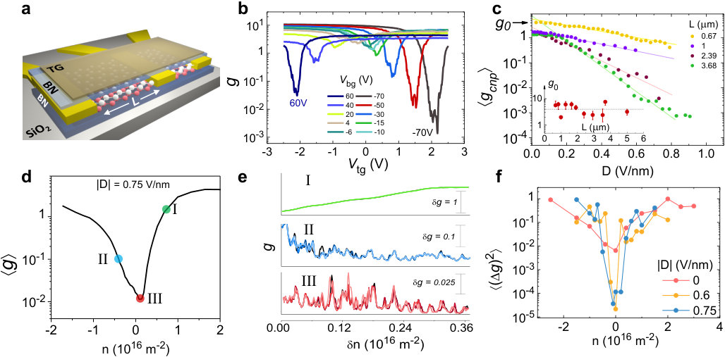 Figure 1
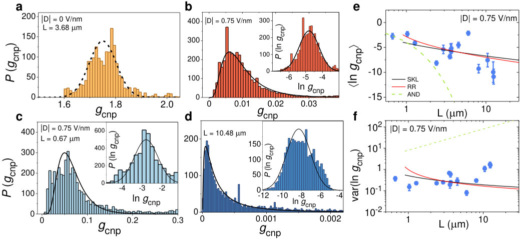 Figure 2
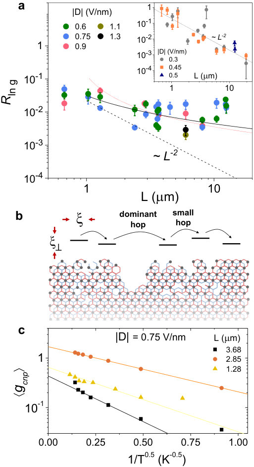 Figure 3
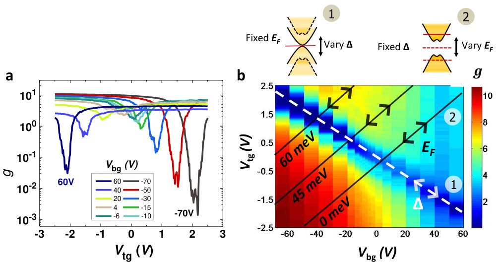 Figure 4
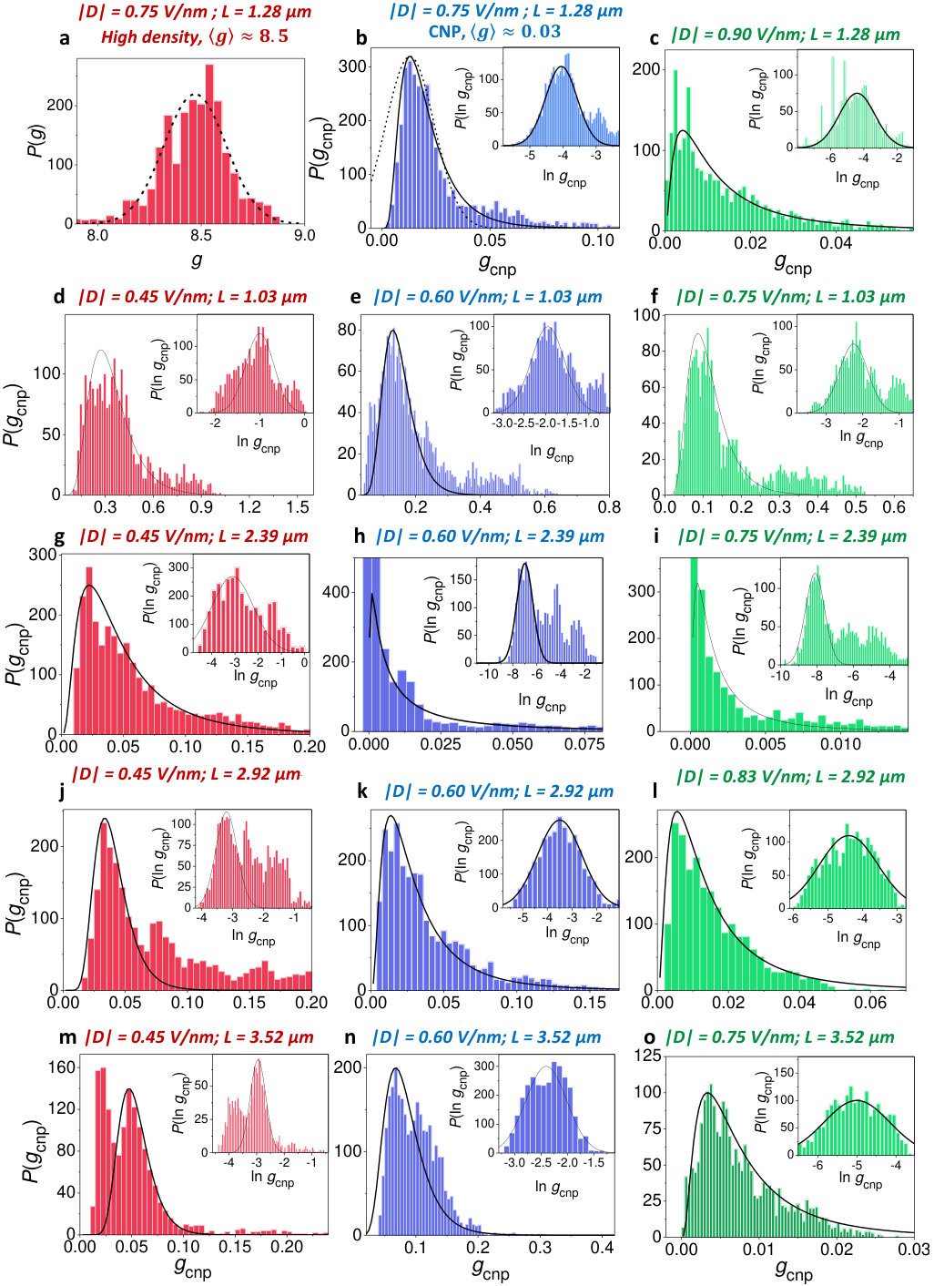 Figure 5
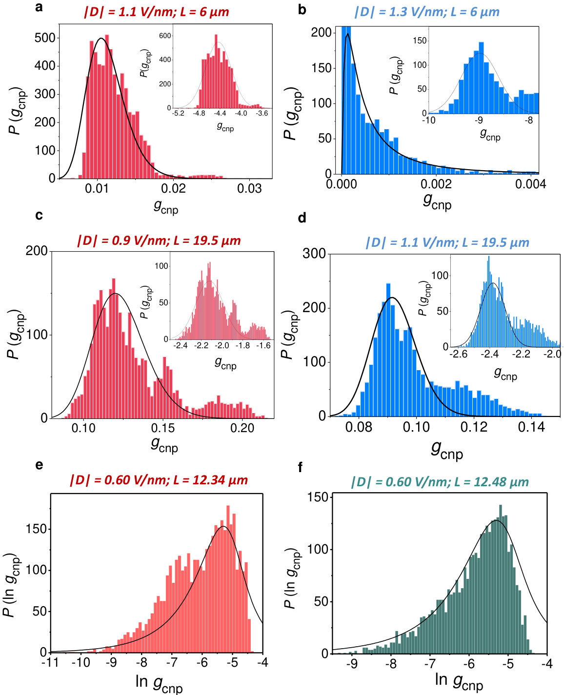 Figure 6
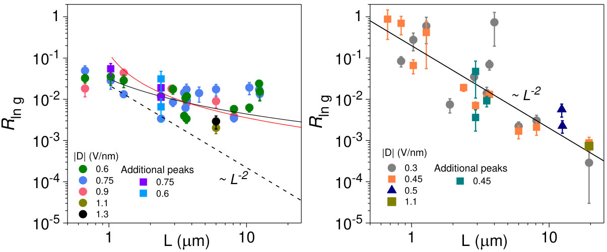 Figure 7
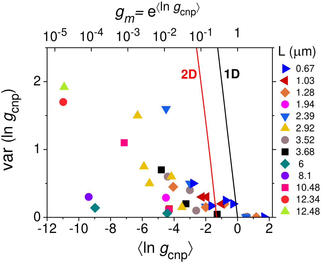 Figure 8
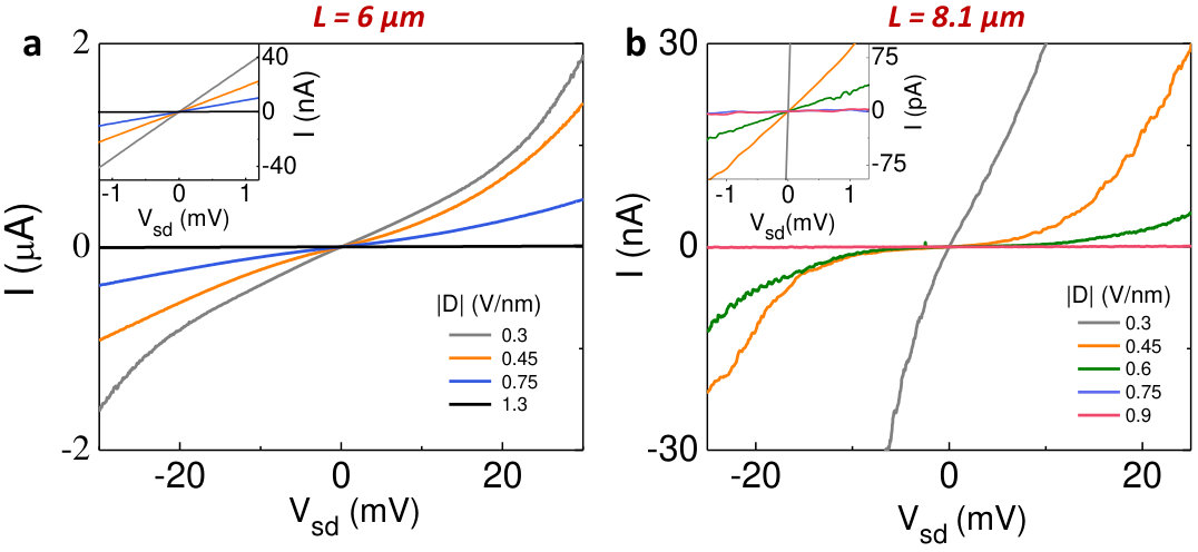 Figure 9
Peer Reviews
No public reviews on file for this paper yet. If you reviewed it on a platform where reviews are public (OpenReview, ICLR, NeurIPS, ICML), you can paste yours below so the community can read it here.
Videos
No videos yet. Explain this paper in a talk, walkthrough, or lecture? Add one.
Supplemental Material: Marginally self-averaging one-dimensional localization in bilayer graphene
Md. Ali Aamir
Department of Physics, Indian Institute of Science, Bangalore 560 012, India.
Paritosh Karnatak
Department of Physics, Indian Institute of Science, Bangalore 560 012, India.
Aditya Jayaraman
Department of Physics, Indian Institute of Science, Bangalore 560 012, India.
T. Phanindra Sai
Department of Physics, Indian Institute of Science, Bangalore 560 012, India.
T. V. Ramakrishnan
Department of Physics, Indian Institute of Science, Bangalore 560 012, India.
Rajdeep Sensarma
Department of Theoretical Physics, Tata Institute of Fundamental Research, Dr. Homi Bhabha Road, Mumbai 400005, India.
Arindam Ghosh
Department of Physics, Indian Institute of Science, Bangalore 560 012, India.
Centre for Nano Science and Engineering, Indian Institute of Science, Bangalore 560 012, India.
.1 Device details
Table below has the details of all the 20 devices we have used in our experiments. The channel length ranges from m to m, varied over an order of magnitude. The channel widths vary over a range from 1m to 3.1m. The mobility range is from cm2/Vs to cm2/Vs.
Table I: Details of all the devices used in this work
Device name Channel Length Channel Width Mobility (cm2/V s) Substrate Contacts type
Dev1 0.67 1.26 1500 SiO2 surface contacted
Dev2 1.03 1.75 5500 BN edge contacted
Dev3 1.28 1.26 1700 SiO2 surface contacted
Dev4 2.39 1.75 5800 BN edge contacted
Dev5 2.85 1.26 1950 SiO2 surface contacted
Dev6 2.92 1.75 4600 BN edge contacted
Dev7 3.52 1.75 5000 BN edge contacted
Dev8 3.6 1.7 16000 BN edge contacted, Hall bar
Dev9 3.66 1.7 16000 BN edge contacted, Hall bar
Dev10 3.68 1.26 3700 SiO2 surface contacted
Dev11 4.52 1.7 16000 BN edge contacted, Hall bar
Dev12 10.48 1.7 16000 BN edge contacted, Hall bar
Dev13 12.34 1.7 16000 BN edge contacted, Hall bar
Dev14 12.48 1.7 16000 BN edge contacted, Hall bar
Dev15 6.0 3.1 15900 BN edge contacted
Dev16 8.1 1.3 10600 BN edge contacted
Dev17 19.51 3.0 10000 BN edge contacted, Hall bar
Dev18 0.84 1 2660 SiO2 surface contacted
Dev19 1.9 1.45 440 SiO2 surface contacted
Dev20 4 2.29 4300 SiO2 surface contacted
.2 Independent control of carrier density and perpendicular electric field using dual-gated device design
Each of the two gates in a dual-gated BLG FET (as shown in Fig. 1a of the main text) contributes independently to the carrier density (as ) and electric field (as ) where is the capacitance per unit area, being the dielectric thickness, is the applied gate voltage and is the gate voltage offset necessary to counterbalance any extrinsic doping. The combined carrier density and electric field is then given by,
[TABLE]
[TABLE]
On fixing one gate, a background carrier density and band gap is fixed which can be tuned continuously using the other gate. Fig. 1b in the main text shows the gate voltage characteristics of the conductance , which has been reproduced in Fig. S1a. The back gate voltage is fixed at several values and the conductance of this device is measured as the top gate voltage is continuously varied. At points where the net carrier density is tuned to zero, called the charge neutrality points (CNP), the conductance takes a minimum value, which we call . As the back gate voltage is changed, its contribution to carrier density is altered and a different is required to neutralise the carrier density to zero. That is why the position of the conductance minimum varies with . Since induced carrier density is proportional to change in the gate voltages (, ) with the corresponding capacitances (, ) as the proportionality factor, the required change in to maintain constant carrier density for a given change in is given by
[TABLE]
also increases as we go further right or left with respect the central trace, because the band gap becomes wider due to increasingly larger perpendicular electric field across the bilayer graphene. The increase is roughly exponential in the magnitude of . The central trace for which is maximum has both the carrier density and band gap closest to zero values, m*-2*, V/nm. The gate voltages at this point , are residual voltages that have counterbalanced residual environmental doping and electric field.
The 2D colour plot of conductance as a function of both and is shown in Fig. S1b. The set of (,) co-ordinates corresponding to CNP, i.e. for zero carrier density but varying electric field, is along the dashed white line running diagonally in the 2D colour plot, and also denoted by label (2). This is a straight line which can be derived by solving the above equations for m*-2*:
[TABLE]
It is clear that the slope of this line for fixed m*-2* is a ratio of the capacitances of the two gates. Similarly, the above equation can be solved for a fixed , which means a fixed band gap, and only varying :
[TABLE]
The (, ) co-ordinates corresponding to three electric fields and V/nm are plotted in Fig. S2b as black lines. Our measurements are performed along such straight lines where both and are varied simultaneously, maintaining a constant electric field (thereby, band gap) and varying carrier density.
.3 Probability distribution functions
Fig. S2 shows conductance probability distribution functions (PDFs) for several channel lengths at various (high) electric fields. Fig. S2a shows the PDF at high carrier density and V/nm for Dev3, where the . Clearly, this PDF can be best fitted with a Gaussian distribution. The variance is of the order of as expected from universal conductance fluctuations, in this weakly disordered metallic regime in BLG. In the same device, when the Fermi level is tuned to the CNP, the PDF shows a log-normal distribution which is made more clear in the insets. This is true for almost all the PDFs that we studied as shown in the Fig. S2b - o, as well as in Fig. 2 in the main text. In some of them (Fig. S2, panels f, h, i, j, m), we find more than one peak that can be fitted with a log-normal distribution of conductance. We have chosen the main or most dominant peak in these panels to compute the statistical properties of , with the expectation that they represent the conductance of the weakest link in the 1D hopping channel. The additional peaks in these cases probably represent other weak links in the path as suggested by the observation that their corresponding values of do not deviate far from that of the main peak, as shown in Fig. S4.
The electric field required to realize strong localization may vary between devices. We observed in Dev15 ( m, m) that the log-normal distribution emerges at 1.3 V/nm. In Dev17 ( m, m) even at 1.1 V/nm the conductance distribution is normal and the device is in a weakly localized regime (see Fig. S4). The corresponding conductance distributions are shown in Fig. S3a - d. We believe, this may be because in a wider device (3 m) there is a larger possibility of bulk channels to shunt the source and drain. Hence, only at larger fields all bulk states gap out and we realize the strongly localized regime. (These bulk channels may arise from local potential fluctuations, or a network of grain boundaries as shown in Ref. Ju2015 ).
In some of the measurements, the PDF of can exhibit weak asymmetry due to blocking effect or “optimal shunts or punctures” between viable localized sites in long and short channels, respectively Raikh1989 ; Hughes1996 . We also have observed this in a few of our results, as shown in Fig. S3e and f, where we have fitted with the RR model in which the distribution function is given by Raikh1989
[TABLE]
where,
[TABLE]
[TABLE]
.4 Variance of as a function of its mean
We have plotted the variance as a function of the mean in Fig. S5. These parameters are extracted from the normal distribution fits to the PDFs. We note that the values of the variance are much lower than numerically predicted for both 1D Beenakker1997 and 2D Somoza2007 disordered systems at K. This further implies the invalidity of the conventional Anderson-like localization, supporting our arguments in the main text. However, at the same time, we also note that traces of vs seem to follow a trend for most of the devices, thereby implying that may be following an approximately universal dependence on with a few exceptions. Thus, it seems that may be sufficient in describing the normal distribution of for most devices. Therefore, the single-parameter scaling hypothesis Kramer1993 may hold in the localization in gapped BLG, statistically speaking, even though Anderson localization is not valid.
.5 Current-Voltage characteristics
characteristics of two devices (Dev15 and Dev16) are shown in Fig. S6. They were measured by performing measurements by AC+DC adder method, followed by numerical integration. We observe a clear non-linear behavior, which is consistent with the presence of an effective transport gap. However, the onset of non-linearity occurs only on a scale of a few mV. Below 1 mV (insets of Fig. S6), the characteristics are linear for all electric fields.
All conductance measurements in this work were carried out with source-drain bias (AC only) ranging from 10 V to 400 V and therefore, within the linear regime. The higher biases were applied in order to improve signal to noise ratio in the measurement of extremely low conductance.
.6 Author contributions
M. A. A., P. K. and A. J. contributed equally to this work. M. A. A., P. K. and A. G. designed the experiment. M. A. A., P. K., A. J. and T. P. S. fabricated the devices. M. A. A., P. K. and A. J. carried out the measurements, and along with A. G. performed the analysis. T. V. R. and R. S. provided the theoretical input. M. A. A., P. K. and A. G. wrote the manuscript with input from all authors.
The reference list from the paper itself. Each links out to its DOI / PubMed record.
- 1(1) Ju, L. et al. Topological valley transport at bilayer graphene domain walls. Nature 520 , 650 (2015).
- 2(2) Raikh, M. E. & Ruzin, I. M. Fluctuations of the hopping conductance of one-dimensional systems. JETP 68, 642 (1989), Zh. Eksp. Teor. Fiz. 95 , 1113 (1989).
- 3(3) Hughes, R. J. F. et al. Distribution-function analysis of mesoscopic hopping conductance fluctuations. Phys. Rev. B 54 , 2091 (1996).
- 4(4) Beenakker, C. W. J. Random-matrix theory of quantum transport. Rev. Mod. Phys. 69 , 731 (1997).
- 5(5) Somoza, A. M., Ortuño, M. & Prior, J. Universal Distribution Functions in Two-Dimensional Localized Systems. Phys. Rev. Lett. 99 , 116602 (2007).
- 6(6) Kramer, B. & Mac Kinnon, A. Localization: theory and experiment. Reports Prog. Phys. 56 , 1469 (1993).