Does the second law hold at cosmic scales?
Manuel Gonzalez-Espinoza, Diego Pav\'on

TL;DR
This paper investigates whether the second law of thermodynamics applies at cosmic scales by analyzing the Hubble factor's history in homogeneous, isotropic universes without relying on specific cosmological models.
Contribution
It provides a purely kinematic analysis to test the validity of the second law at large cosmological scales, independent of curvature or model assumptions.
Findings
Supports the applicability of the second law at cosmic scales
Shows the law holds regardless of spatial curvature
Uses a model-independent, kinematic approach
Abstract
The second law of thermodynamics is known to hold at small scales also when gravity plays a leading role, as in the case of black holes and self-gravitating radiation spheres. It has been suggested that it should as well at large scales. Here, by a purely kinematic analysis \textemdash based on the history of the Hubble factor and independent of any cosmological model \textemdash , we explore if this law is fulfilled in the case of homogeneous and isotropic universes regardless of the sign of the spatial curvature.
Click any figure to enlarge with its caption.
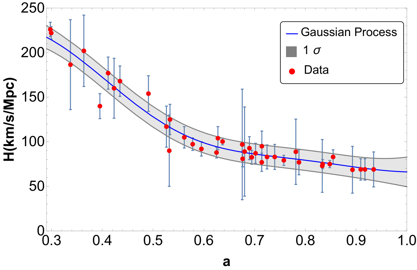 Figure 1
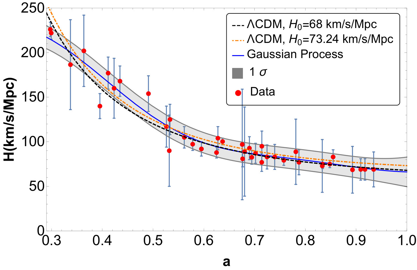 Figure 2
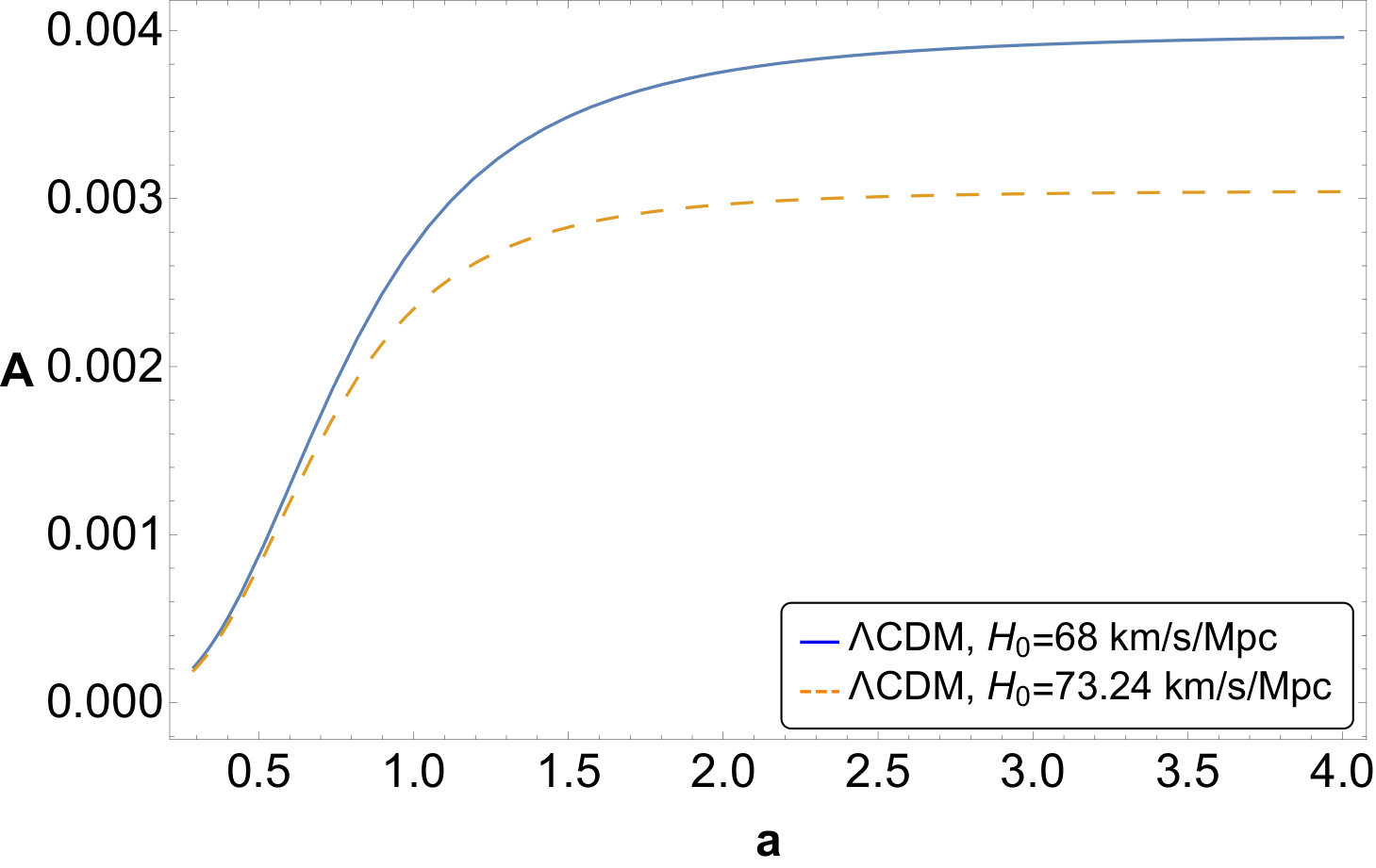 Figure 3
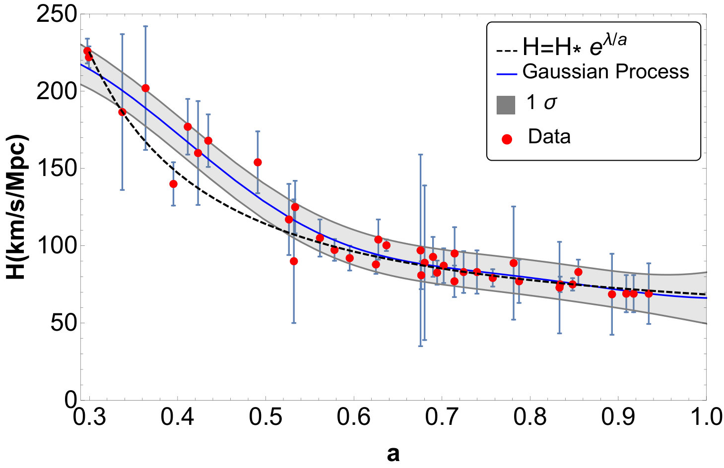 Figure 4
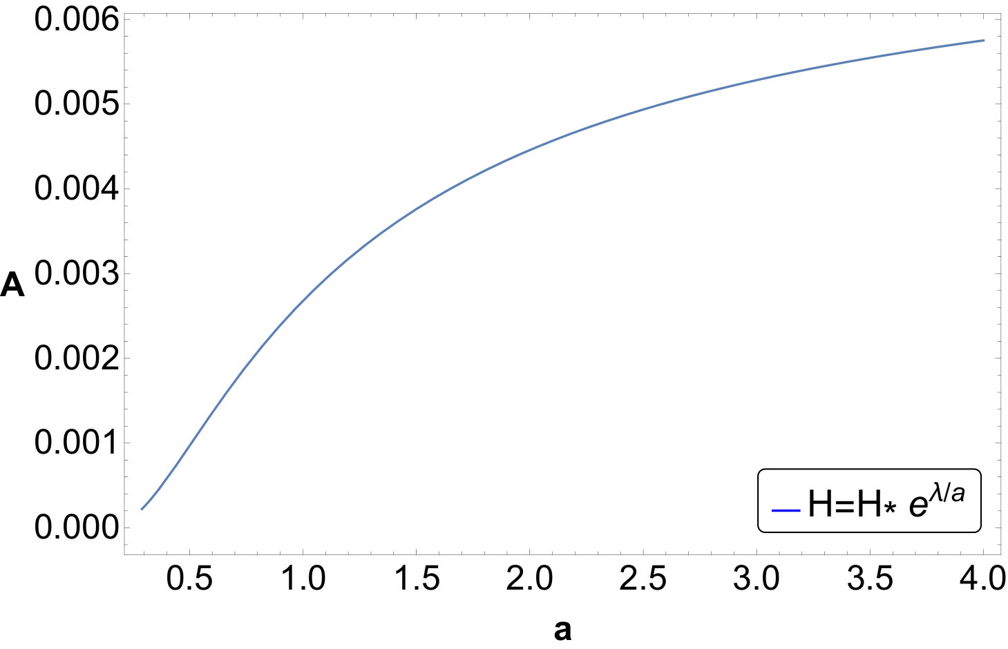 Figure 5
 Figure 6
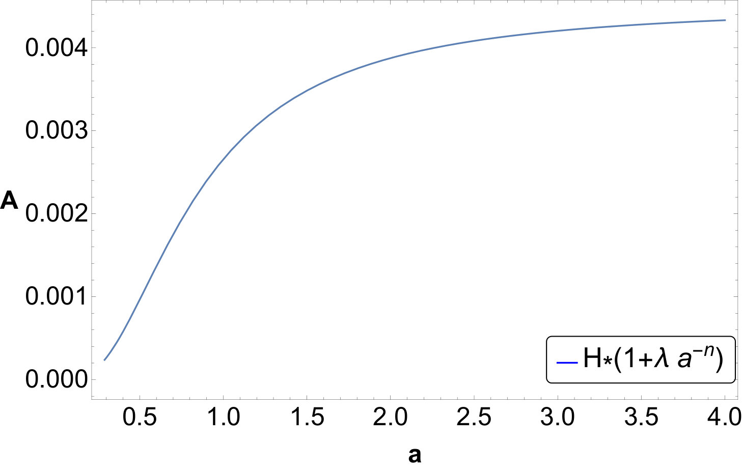 Figure 7
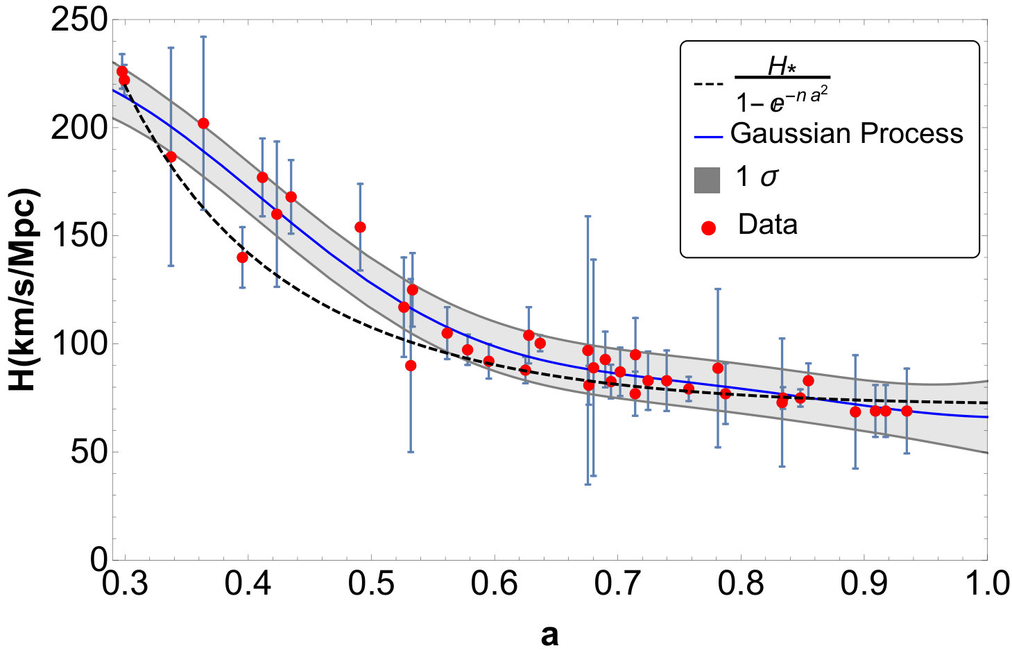 Figure 8
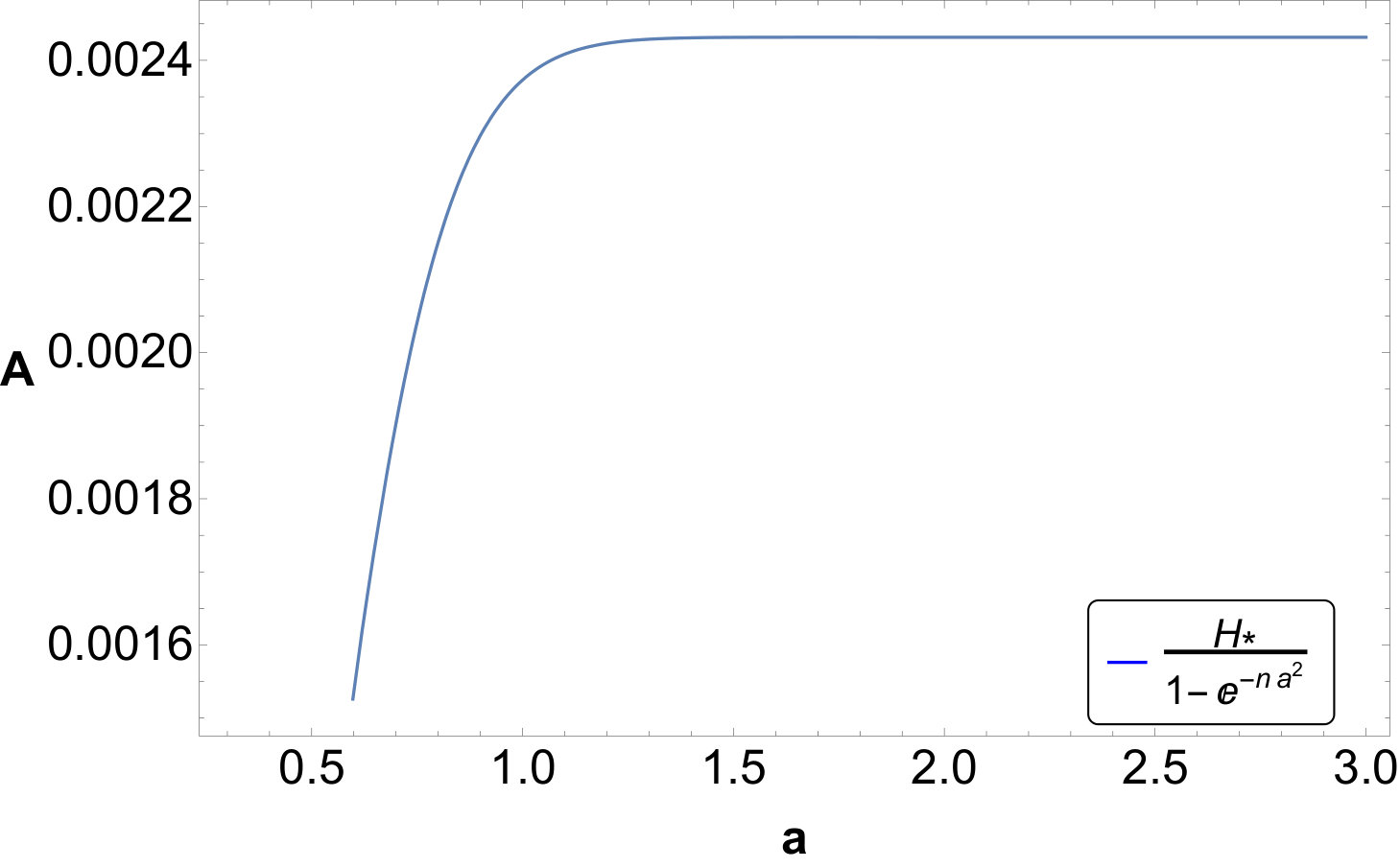 Figure 9
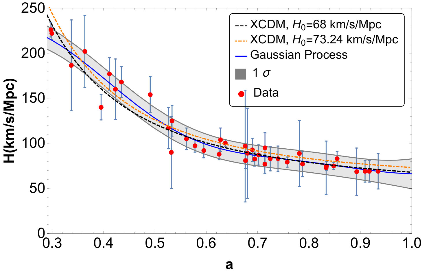 Figure 10
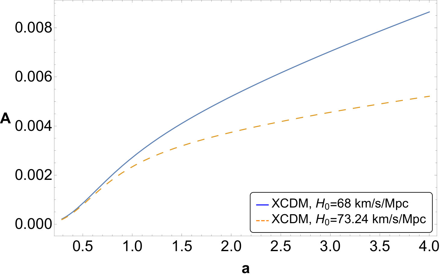 Figure 11
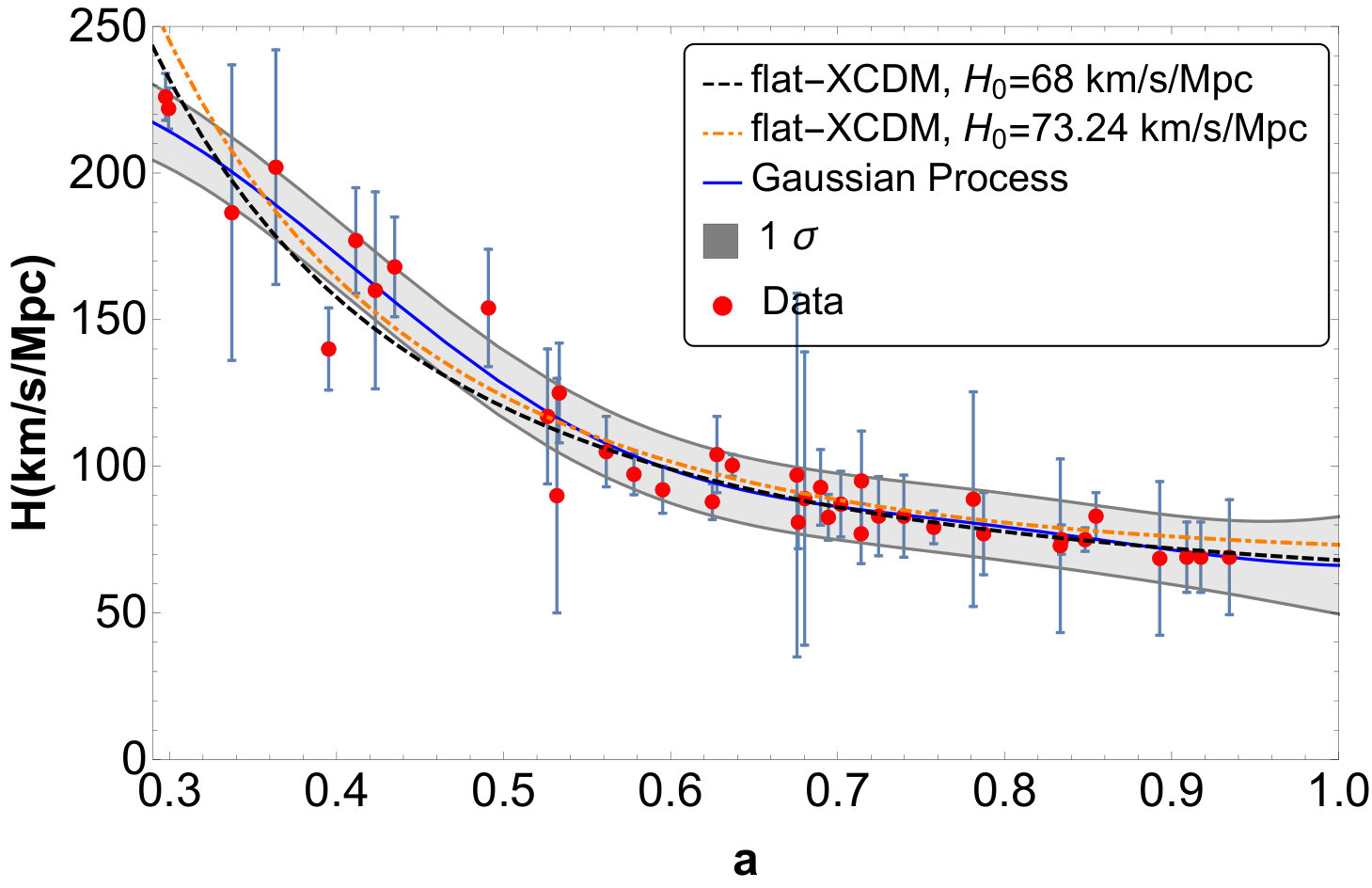 Figure 12
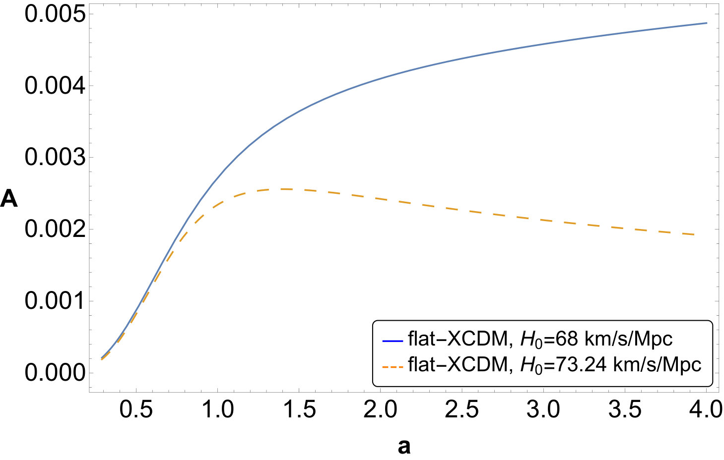 Figure 13
| (km s-1 Mpc-1) | Ref. | ||
|---|---|---|---|
| Zhang et al. (2014) | |||
| Simon et al. (2005) | |||
| Simon et al. (2005) | |||
| Zhang et al. (2014) | |||
| Simon et al. (2005) | |||
| Moresco et al. (2012) | |||
| Moresco et al. (2012) | |||
| Zhang et al. (2014) | |||
| Simon et al. (2005) | |||
| Zhang et al. (2014) | |||
| Cuesta et al. (2016) | |||
| Moresco et al. (2012) | |||
| Moresco et al. (2012) | |||
| Simon et al. (2005) | |||
| Moresco et al. (2012) | |||
| Moresco et al. (2012) | |||
| Blake et al. (2012) | |||
| Moresco et al. (2012) | |||
| Ratsimbazafy et al. (2017) | |||
| Moresco et al. (2012) | |||
| Stern et al. (2010) | |||
| Cuesta et al. (2016) | |||
| Moresco et al. (2012) | |||
| Blake et al. (2012) | |||
| Moresco et al. (2012) | |||
| Blake et al. (2012) | |||
| Moresco et al. (2012) | |||
| Moresco et al. (2012) | |||
| Stern et al. (2010) | |||
| Simon et al. (2005) | |||
| Moresco et al. (2012) | |||
| Simon et al. (2005) | |||
| Moresco (2015) | |||
| Simon et al. (2005) | |||
| Simon et al. (2005) | |||
| Simon et al. (2005) | |||
| Moresco (2015) | |||
| Delubac et al. (2015) | |||
| Font-Ribera et al. (2014) |
Peer Reviews
No public reviews on file for this paper yet. If you reviewed it on a platform where reviews are public (OpenReview, ICLR, NeurIPS, ICML), you can paste yours below so the community can read it here.
Videos
No videos yet. Explain this paper in a talk, walkthrough, or lecture? Add one.
Does the second law hold at cosmic scales?
Manuel Gonzalez-Espinoza,1 Diego Pavón2
1Instituto de Física, Pontificia Universidad Católica de Valparaíso, Casilla 4950, Valparaíso, Chile.
2Departamento de Física, Universidad Autónoma de Barcelona, 08193 Bellaterra, Barcelona, Spain E-mail: [email protected]: [email protected]
(Accepted XXX. Received YYY; in original form ZZZ)
Abstract
The second law of thermodynamics is known to hold at small scales also when gravity plays a leading role, as in the case of black holes and self-gravitating radiation spheres. It has been suggested that it should as well at large scales. Here, by a purely kinematic analysis —based on the history of the Hubble factor and independent of any cosmological model —, we explore if this law is fulfilled in the case of homogeneous and isotropic universes regardless of the sign of the spatial curvature.
keywords:
cosmology:theory – gravitation
††pubyear: 2018††pagerange: Does the second law hold at cosmic scales?–Does the second law hold at cosmic scales?
1 Introduction
At first sight, gravity and thermodynamics appear as practically disjoint, if not altogether unrelated, branches of Physics. However, as a closer look reveals, this is misleading. Recall, for instance, Tolman’s law of thermodynamic equilibrium in a stationary gravitational field (Tolman, 1930, 1934), Unruh’s effect (Unruh, 1976), the entropy associated to event (Hawking, 1975, 1976; Wald, 1994; Gibbons & Hawking, 1977) and apparent horizons, (Bak & Rey, 2000; Cai & Cao, 2007), the generalized second law of thermodynamics for black holes (Bekenstein, 1974, 1975), the equilibrium of self-gravitating radiation spheres (Sorkin et al., 1981; Pavón & Landsberg, 1988), and, finally, the realization that the field equations of Einstein gravity can be understood as thermodynamic equations of state (Jacobson, 1995; Padmanabhan, 2005).
Therefore, the question arises: is the Universe a thermodynamic system? To put it another way, does it follow the laws of thermodynamics? In general relativity, and in most theories of gravity, the conservation of energy, —i.e., the first law —emerges directly from the field equations of the theory in question, but to experimentally verify whether or not it is fulfilled at large scales appears far beyond present human capability. Here, we do not concern ourselves with this law; we simply assume its validity. As for the third law, we think it does not apply at large scales since the concept of “temperature of the universe" has no clear meaning. It is the second law that we are interested in.
At this point we feel expedient to recall it. As we witness on daily basis, macroscopic systems tend spontaneously to thermodynamic equilibrium. This is at the very basis of the second law. The latter encapsulates this by asserting that the entropy, , of isolated systems never decreases, and that, at least in the last stage of approaching equilibrium, it is concave, (Callen, 1960). The prime means derivative with respect to the relevant thermodynamic variable. In this paper we shall tentatively apply this to cosmic expansion.
Before going any further, we wish to emphasize that sometimes the second law is found formulated by stating just the above condition on but not on . While this mutilated version works well for many practical purposes, it is insufficient in general. Otherwise one would observe systems whose entropy increased without bound, which is at odds with daily experience. In this connection, it should be noted that this can arise in Newtonian gravity. A case in point is the gravothermal catastrophe: The entropy of a number of gravitating point masses confined to the interior of a rigid sphere, of perfectly reflecting walls, whose radius exceeds some critical value, diverges (Antonov, 1962; Lynden-Bell et al., 1968). This uncomfortable outcome hints that thermodynamics and Newtonian gravity are not fully consistent with each other. Nevertheless, it can be evaded by resorting to general relativity: The formation of a black hole at the center of the sphere renders the entropy of the system to stay bounded.
Today, it is widely agreed that the entropy of the universe (we mean that part of the universe in causal contact with us) is overwhelmingly contributed by the entropy of the cosmic horizon (about times the Boltzmann constant). Supermassive black holes and the cosmic microwave radiation, alongside the cosmic sea of neutrinos, come behind by and orders of magnitude, respectively. All the other sources of entropy contribute much less (Egan & Lineweaver, 2010). Therefore, to ascertain whether the universe fulfills the second law it suffices to see whether the entropy of the cosmic horizon, , comply with and . In homogeneous and isotropic universes one can define different causal horizons. We are interested in the apparent horizon (the boundary hyper-surface of the spacetime anti-trapped region Bak & Rey (2000)), since it always exists in non-static universes, independently of whether it accelerates when or not. Neglecting possible (small) quantum corrections, the entropy of the horizon is found to be proportional to the area of the latter (Bak & Rey, 2000; Cai & Cao, 2007)
[TABLE]
where , the radius of the apparent horizon, the normalized spatial curvature parameter, and the Planck’s length. Thereby, it follows that the universe will comply with the second law provided that and (the prime means derivative with respect the scale factor of the Robertson-Walker metric).
The aim of this paper is to explore whether this is to be expected in view of the current data of the history of the Hubble factor. As it turns out, our study —which is purely kinematic —suggests that this may well be the case and, i.e., that the universe seems to tend to a state of maximum entropy in the long run. This outcome was suggested earlier (Ferreira & Pavón, 2016). Here we strengthen this suggestion by employing an ampler dataset and using a somewhat different analysis.
This result is also achievable from the "holographic equipartition principle", that the rate at which the three-spatial volume of the flat universe increases with expansionn is proportional to the difference of the number of degrees of freedom between the horizon and the bulk (Krishna & Mathew, 2017). However, our approach is more economical as we neither use temperatures at all nor assume equality beween them.
The paper is organized as follows. Next section presents the observational data and the best fit to them. Section III introduces three simple parametrizations of the Hubble function in terms of the scale factor. As we will see, the derivatives of the area of the apparent horizon associated to these parametrizations fulfill the inequalities expressed in the preceding paragraph. Section IV studies, for the sake of comparison, the evolution of the apparent horizon for a handful of cosmological models that are known to fit reasonably well the data. Last section presents our conclusions and final comments.
2 data and Gaussian Process
We shall use the set of data of the Hubble factor, , alongside their confidence interval, in terms of the redshift, compiled by Farooq et al. (2017) and Ryan et al. (2018), listed in table 1. These data come from different sources, also listed there, and were obtained using differential ages of red luminous galaxies, galaxy clustering and baryon acoustic oscillation techniques —see references in the said table for details. Our study does not rely on any cosmological model at all. However, in section IV, we compare the predictions of some successful models about the evolution of the area of the horizon with the outcome of our kinematic analysis.
Regrettably, a few of data are affected by uncomfortably big confidence intervals whereby some statistically-based smoothing process must be applied to the whole dataset if one wishes to draw sensible conclusions. We resort to the machine learning model Gaussian process, which infers a function from labelled training data (Rasmussen & Williams, 2006). This process is capable of capturing a wide range of behaviours with only a set of parameters and admit a Bayesian interpretation (Zhao, 2018). In this study we are implementing the Gaussian process using the Wolfram Language (which includes a wide range machine learning capabilities) to be more specific we are using the Predict function with the Performance Goal based on Quality. All the numeric analysis is only based on the library given by the Wolfram Mathematica 10.4. See Seikel et al. (2012) for a deep numerical analysis, with useful references, to this technique in a cosmological context.
Application of the Gaussian process to the dataset results in the blue solid line —the "best fit" —and its (gray shaded) confidence band, in terms of the scale factor, as shown in Fig. 1. Extrapolation to gives km/s/Mpc. This line suggests that is negative in the whole interval and that is positive for . Inspection of Figs. 1(c) and 3(a) of Carvalho & Alcaniz (2011) also supports this view. In principle there is no grounds to believe that this should be different for .
Notice that implies (at least, in spatially flat universes). Likewise, leads to , which must be realized from some scale factor onwards if the entropy of the horizon is to approach a maximum in the long run (alongside ). As we will see below, in this regard, the impact of the spatial curvature will have little consequence (if at all) at late times.
3 Parameterizing the Hubble function
Here we essay three simple parametrizations of that comply with the conditions and , mentioned above, in the interval covered by the data listed in table 1, and that lead to and (the latter inequality is not necessarily valid when ). We emphasize that these three Hubble functions are not meant to describe cosmic expansion for , but we hope they will be qualitatively correct otherwise. We will contrast them with the best fit (blue solid line) shown in Fig. 1. We will take as the “goodness" of a given parametrization the area enclosed by the said best fit line and the graph of the parametrization (the smaller the area, the better the parametrization).
3.1 Parametrization 1
Our first proposal is
[TABLE]
By numerically fitting it to the best fit line with the confidence interval of Fig. 1, one obtains for the free parameters: km/s/Mpc and . Then, km/s/Mpc, and the age of the universe, defined as , is Gyr. On the other hand, the deceleration parameter, , evaluated at present gives and the transition deceleration-acceleration occurs at . The area between the graph of the parametrization and the blue solid line (best fit) obtained using the Gaussian Process is .
Figure 2 contrasts Eq. (2), black dashed line, with the best fit to the Hubble data. The dependence of the area of the apparent horizon on the scale factor for is depicted in Fig. 3. The graphs for and show no significant difference with this one; all three are practically coincident (this is also true for parametrizations 2 and 3 considered below). From this graph we learn that in the range of scale factor considered and that from onward.
3.2 Parametrization 2
The second parametrization is
[TABLE]
Proceeding as in the previous case, the best fit for the free parameters are found to be: km/s/Mpc, and . Thus, Gyr, km/s/Mpc, and . Figure 4 compares this parametrization (black dashed line) with the best fit to the Hubble data. The area between the curves is . Figure 5 shows the evolution of the area of the apparent horizon.
3.3 Parametrization 3
As third parametrization, we propose
[TABLE]
Proceeding as before yields, km/s/Mpc and . Thus, Gyr, km/s/Mpc, , and . Figure 6 contrasts the graph (black dashed line) corresponding to Eq. (4) with the best fit to the Hubble data. The area between the curves is . Figure 7 shows the evolution of the area of the horizon.
[TABLE]
The value for derived from these three essay Hubble functions is quite consistent with the one measured by Daly et al. (2008) () by a model independent analysis. These authors based their study on the distances and redshifts to 192 supernovae, 30 radiogalaxies and 38 galaxy clusters. However, the quantity that follow from the said Hubble functions results slightly lower than the obtained by Daly et al., namely .
All three parametrizations share the features that, regardless the sign of the curvature index , the area, , of the apparent horizon never decreases and that from some value of the scale factor on. This hints that the universe described by each of them fulfills the second law of thermodynamics and tend asymptotically to state of maximum entropy of the order of in Planck units.
Nevertheless, Hubble functions that comply with and but fail to lead to , at late times (at least when ) can be proposed. Consider for instance and where is a positive definite constant. The entropy of spatially-flat cosmological models whose expansion were governed by any of these two functions would increase unbounded to never reach a state of thermal equilibrium. However, as previously remarked (Pavón & Radicella, 2013), both Hubble functions are at stark variance with observation. The first one corresponds to a universe that never accelerates. The second one to a universe that accelerates at early times (i.e., for ) and decelerates forever afterward.
At this point one may wonder whether the evolution of the apparent horizon dictated by the three Hubble’s essay functions of above are qualitatively consistent with the corresponding evolution predicted by those cosmological models that fit reasonably well the observational data. This will be the subject of the next section. As it will turn out, the answer to this question is in the affirmative.
4 Cosmological models dominated pressureless matter and dark energy
In this section we briefly consider the evolution of the area of the apparent horizon in a homogeneous and isotropic universe governed by Einstein gravity and dominated by pressureless matter (baryonic plus dark) and dark energy. We also allow for the presence of a small spatial curvature. We first study the case in which dark energy is in the form of a positive cosmological constant, , and then when it is given by a scalar field with constant equation of state parameter . In both cases we assume, in agreement with dynamical measurements (see e.g., Freedman (2001) for a short review and §V in Bartelmann (2010)), that the matter component contributes to the total energy budget by about 30 per cent. The rest is in the form of dark energy (either a cosmological constant or a scalar field) plus spatial curvature. As stressed in Ryan et al. (2018); Ooba et al. (2017); Park & Ratra (2018a, b) the latter may well be non-negligible.
Nowadays there is a discrepancy between local and global measurements of the Hubble constant, . The former yield km/s/Mpc (Riess et al., 2016) while the latter, based on the spatially flat CDM model, give km/s/Mpc (Ade, 2016). Below, we will use in turn the result of Riess as well as the prior km/s/Mpc employed by Ryan et al. (2018). As we will see, no major difference arise with regard to the overall evolution of the area of the horizon. At any rate, both values are somewhat above the best fit obtained by the Gaussian Process (blue solid line in Fig. 1). As input data we will employ the cosmological parameter values obtained in Ryan et al. (2018) by constraining several simple cosmological models based in Einstein gravity (both with and without spatial curvature) using 31 data in the redshift range and 11 baryon acoustic oscillation distance measurements.
4.1 CDM models
For this kind of models Friedamann’s equation reads
[TABLE]
where and denote the present value of the density parameters of matter and spatial curvature, respectively, and the parameter density associated to the cosmological constant. From (5) it is seen that at large times the area of the apparent horizon is of the order of .
We study two CDM cases:
- •
First case, km/s/Mpc, and (see black dashed line in Fig. 8). Thus, Gyr, and . The area between the curves is .
- •
Second case, km/s/Mpc, and (see orange dot-dashed line in Fig. 8). Thus, Gyr, and . The area between the curves is .
The evolution of the area of the apparent horizon is shown, in each case, in Fig. 9.
4.2 flat-XCDM models
We consider a generic dark energy model that, from the phenomenological viewpoint, essentially differs at first order from the CDM in that the equation of state parameter, , is a constant different from . We study in turn two flat-XCDM cases where
[TABLE]
- •
First case, km/s/Mpc, and (see black dashed line in Fig. 10). Thus, Gyr, and . The area between the curves is .
- •
Second case, km/s/Mpc, and (see orange dot-dashed line in Fig. 10). Thus, Gyr, and . The area between the curves is . Note —see Fig. 11 —that the area of the apparent horizon begins increasing but at some point (as soon as the dark energy takes over) it decreases. This violation of the second law (which occurs because, in this case, the dark energy is of “phantom" type, ) goes hand in hand with the fact that phantom fields present classical (Dabrowski, 2015) and quantum instabilities (Cline et al., 2004; Sbisà, 2014) that render them implausible.
In both cases the evolution of the area of the horizon is shown Fig. 11.
4.3 Non-flat XCDM models
The Hubble factor of spatially curved XCDM models can be written as
[TABLE]
[TABLE]
- •
First case, km/s/Mpc, , and (see black dashed line in Fig. 12). Thus, Gyr, and . The area between the curves is .
- •
Second case, km/s/Mpc, , , (see orange dot-dashed line in Fig. 12). Thus, Gyr, and . The area between the curves is .
The evolution of the area of the apparent horizons is depicted in Fig. 13.
Notice that the cosmological models considered in this section fit better (by about a factor of 2) the best fit (blue solid line) to the Hubble’s data set in Fig. 1 than any of the three parametrizations of section 3 (i.e., the former have a lower value for the area between the curves than the latter) even though no fitting process to the said data has been applied to the cosmological models. This was to be expected with regard to the Hubble essay functions 1 and 3 because the models of this section have one or two more free parameters.
We have just considered a handful of simple cosmological models that fit observation reasonably well —see Ref. Ryan et al. (2018). More sophisticated models, as those beyond Einstein gravity, also deserve consideration. However, generally speaking, in that case the fit of the model parameters to the observational data is significantly affected by systematics.
We conclude this section by noting that the apparent horizon of homogeneous and isotropic cosmological models, regardless of their spatial curvature, that fit current observation and are classical and quantum-mechanically stable comply with the same conditions ( and , the latter at least from some value of the scale factor onward) than the three essay Hubble functions (Eqs. (2), (3) and (4)) of section III. These two conditions ensure that the corresponding cosmological model respects the second law. This suggests that from this preliminary dataset, however scarce and of limited quality, one may glimpse that the universe fulfills the said law. Therefore, from this point of view, it appears to behave as a normal thermodynamic system. Recently, this conclusion was also attained by an altogether different route, namely by the analysis of the statistical fluctuations of the flux of energy on the apparent horizon (Mimoso & Pavón, 2018). As it turns out, the strength of the fluctuations decrease with the area of the horizon and increase with the temperature of the latter. Just as in systems in which gravity is absent (Landau & Lifshitz, 1971).
5 Concluding remarks
The recent years have witnessed a reinforcement of the connection between gravity and thermodynamics. As two salient landmarks we mention the discovery that fully gravitationally collapsed objects possess a well defined temperature and entropy (Hawking, 1975, 1976), and the realization that the gravity field equations can be viewed as thermodynamic equations of state (Jacobson, 1995; Padmanabhan, 2005). In this context it is natural to ask whether the universe behaves as a normal thermodynamic system; that is to say, whether it satisfies the laws of thermodynamics; most importantly the second law. Actually, this amount to consider whether the aforesaid law also holds at cosmic scales.
To answer this question we assumed the universe homogeneous and isotropic at sufficiently large scales and, based on the history of the Hubble function as specified in table 1, made a kinematic analysis independent of any cosmological model. In section II, by applying the Gaussian Process we obtained a best fit to the data (blue solid line in Fig. 1). The latter suggests that and . Then, in section III we essayed three simple Hubble functions (Eqs. (2), (3) and (4)) that comply with these two inequalities, and are consistent with the second law as applied to the area of the apparent horizon (i.e., and ), and reproduce reasonably well (especially for ) the best fit to the Hubble data —Figs. 2, 4 and 6. As illustrated by two examples, Hubble functions that imply in the long run strongly disagree with observation at the background level. In section IV we contrasted the evolution of the Hubble function predicted by some simple, flat as well as non-flat, cosmological models that fit observation reasonably well (Ryan et al., 2018) with the best fit to the Hubble dataset (Figs. 8, 10 and 12). These fits are only somewhat better than those of the three parametrizations proposed in section III. Except for the second flat-XCDM model, that is of “phantom" type and presents instabilities at the classical and quantum level, the area of the apparent horizon is always increasing and with second derivative negative in the long run. In this regard, it mimics the evolution of the area of the apparent horizon associated to the three essay Hubble functions of section III.
Our overall conclusion is that the second law of thermodynamics seems to be obeyed by the universe we observe today and, therefore, that this law also holds at cosmic scales. However, this conclusion, extracted from a scarce number of Hubble data of not great quality, cannot be but preliminary. Nevertheless, we hope that in the not distant future a much more ample set of data of better quality will be available whence we will make able to reach a firmer conclusion. This improvement in the quality and number of data may arise not only from a refinement of the current techniques but also from measuring the drift of the redshift of distant sources (Sandage, 1962; Loeb, 1998). This seems feasible thanks to the future European Extreme Large Telescope alongside advanced spectographs like CODEX (2018).
Finally, as is apparent, our approach is purely classical in nature. Nevertheless, it is worthy to emphasize that it is also robust against quantum fluctuations since, as demonstrated by Oshita (2018), these do not invalidate the generalized second law because cosmological decoherence prevents it in the case of de Sitter expansion.
Acknowledgements
M. G.-E. acknowledges support from a PUCV doctoral scholarship and DI-VRIEA-PUCV for financial support.
The reference list from the paper itself. Each links out to its DOI / PubMed record.
- 1Ade (2016) Ade P., 2016, A&A, 594, A 13
- 2Antonov (1962) Antonov V., 1962, Vest. Leningr. Gos. Univ., 7, 135
- 3Bak & Rey (2000) Bak D., Rey S.-J., 2000, Class. Quantum Grav., 17, L 83
- 4Bartelmann (2010) Bartelmann M., 2010, Rev. Mod. Phys., 82, 331
- 5Bekenstein (1974) Bekenstein J. D., 1974, Phys. Rev. D, 9, 3292
- 6Bekenstein (1975) Bekenstein J. D., 1975, Phys. Rev. D, 12, 3077
- 7Blake et al. (2012) Blake C., et al., 2012, Mon. Not. R. Astron. Soc., 425, 405
- 8CODEX (2018) CODEX 2018, An ultra-stable, high-resolution optical spectrograph for the E-ELT, www.iac.es/proyecto/codex