Routing in Histograms
Man-Kwun Chiu, Jonas Cleve, Katharina Klost, Matias Korman, and Wolfgang Mulzer, Andr\'e van Renssen, Marcel Roeloffzen, Max, Willert

TL;DR
This paper develops efficient routing schemes within specific geometric graph structures called histograms, achieving near-optimal path lengths with minimal label and table sizes.
Contribution
It introduces new routing algorithms for simple and double histograms, providing optimal or near-optimal path routing with small labels and tables.
Findings
Routing in double histograms achieves paths at most twice the shortest path length.
Routing in simple histograms achieves optimal path lengths.
Labels and routing tables are of size O(log n) bits.
Abstract
Let be an -monotone orthogonal polygon with vertices. We call a simple histogram if its upper boundary is a single edge; and a double histogram if it has a horizontal chord from the left boundary to the right boundary. Two points and in are co-visible if and only if the (axis-parallel) rectangle spanned by and completely lies in . In the -visibility graph of , we connect two vertices of with an edge if and only if they are co-visible. We consider routing with preprocessing in . We may preprocess to obtain a label and a routing table for each vertex of . Then, we must be able to route a packet between any two vertices and of , where each step may use only the label of the target node , the routing table and neighborhood of the current node, and the packet header. We present a routing scheme for double…
Click any figure to enlarge with its caption.
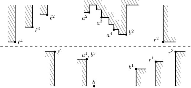 Figure 1
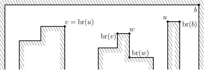 Figure 2
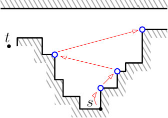 Figure 3
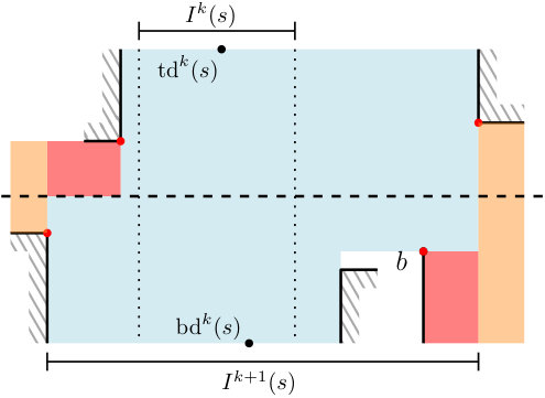 Figure 4
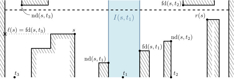 Figure 5
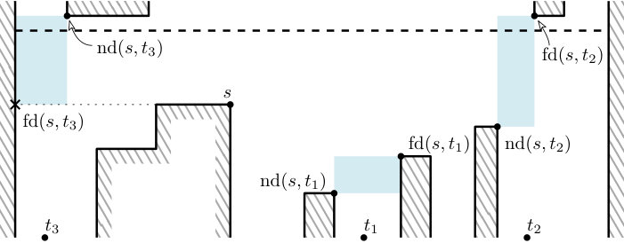 Figure 6
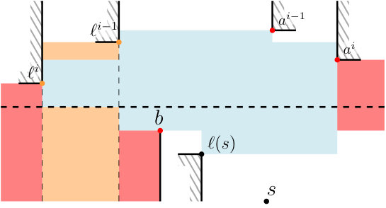 Figure 7
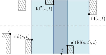 Figure 8
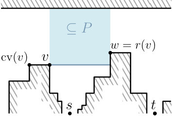 Figure 9
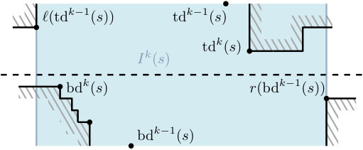 Figure 10
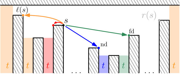 Figure 11
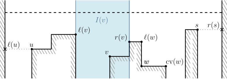 Figure 12
Peer Reviews
No public reviews on file for this paper yet. If you reviewed it on a platform where reviews are public (OpenReview, ICLR, NeurIPS, ICML), you can paste yours below so the community can read it here.
Videos
No videos yet. Explain this paper in a talk, walkthrough, or lecture? Add one.
Routing in Histograms111
MC was supported by JST ERATO Grant Number JPMJER1201 (Japan) and ERC STG 757609. JC was supported by ERC STG 757609 and DFG grant MU 3501/1-2. MK was supported by MEXT KAKENHI No. 17K12635 and the NSF award CCF-1422311. WM was supported in part by ERC StG 757609. AvR and MR were supported by JST ERATO Grant Number JPMJER1201, Japan.
Man-Kwun Chiu
Institut für Informatik, Freie Universität Berlin, Germany
{chiumk,jonascleve,kathklost,mulzer,willerma}@inf.fu-berlin.de
Jonas Cleve
Institut für Informatik, Freie Universität Berlin, Germany
{chiumk,jonascleve,kathklost,mulzer,willerma}@inf.fu-berlin.de
Katharina Klost
Institut für Informatik, Freie Universität Berlin, Germany
{chiumk,jonascleve,kathklost,mulzer,willerma}@inf.fu-berlin.de
Matias Korman
Department of Computer Science, Tufts University, Medford, MA, USA
Wolfgang Mulzer
Institut für Informatik, Freie Universität Berlin, Germany
{chiumk,jonascleve,kathklost,mulzer,willerma}@inf.fu-berlin.de
André van Renssen
School of Computer Science, University of Sydney, Sydney, Australia
Marcel Roeloffzen
Department of Mathematics and Computer Science, TU Eindhoven, Eindhoven, the Netherlands
Max Willert
Institut für Informatik, Freie Universität Berlin, Germany
{chiumk,jonascleve,kathklost,mulzer,willerma}@inf.fu-berlin.de
Abstract
Let be an -monotone orthogonal polygon with vertices. We call a simple histogram if its upper boundary is a single edge; and a double histogram if it has a horizontal chord from the left boundary to the right boundary. Two points and in are co-visible if and only if the (axis-parallel) rectangle spanned by and completely lies in . In the -visibility graph of , we connect two vertices of with an edge if and only if they are co-visible.
We consider routing with preprocessing in . We may preprocess to obtain a label and a routing table for each vertex of . Then, we must be able to route a packet between any two vertices and of , where each step may use only the label of the target node , the routing table and neighborhood of the current node, and the packet header.
We present a routing scheme for double histograms that sends any data packet along a path whose length is at most twice the (unweighted) shortest path distance between the endpoints. In our scheme, the labels, routing tables, and headers need bits. For the case of simple histograms, we obtain a routing scheme with optimal routing paths, -bit labels, one-bit routing tables, and no headers.
1 Introduction
The routing problem is a classic question in distributed graph algorithms [16, 23]. We have a graph and would like to preprocess it for the following task: given a data packet located at some source vertex of , route the packet to a target vertex of , identified by its label. The routing should have the following properties: (A) locality: to determine the next step of the packet, it should use only information at the current vertex or in the packet header; (B) efficiency: the packet should travel along a path whose length is not much larger than the length of a shortest path between and . The ratio between the length of this routing path and a shortest path is called the stretch factor; and (C) compactness: the space requirements for labels, routing tables, and packet headers should be small.
Obviously, we could store at each vertex of the complete shortest path tree of . Then, the routing scheme is perfectly efficient: we can send the packet along a shortest path. However, the scheme lacks compactness. Thus, the challenge is to balance the (seemingly) conflicting goals of compactness and efficiency.
There are many compact routing schemes for general graphs [1, 2, 12, 13, 14, 24, 25]. For example, the scheme by Roditty and Tov [25] needs to store a poly-logarithmic number of bits in the packet header and it routes a packet from to on a path of length O\big{(}k\Delta+m^{1/k}\big{)}, where is the shortest path distance between and , is any fixed integer, is the number of nodes, and is the number of edges. The routing tables use space. In the late 1980’s, Peleg and Upfal [23] proved that in general graphs, any routing scheme with constant stretch factor must store bits per vertex, for some constant . Thus, it is natural to focus on special graph classes to obtain better routing schemes. For instance, trees admit routing schemes that always follow the shortest path and that store bits at each node [15, 26, 28]. Moreover, in planar graphs, for any fixed , there is a routing scheme with a poly-logarithmic number of bits in each routing table that always finds a path that is within a factor of from optimal [27]. Similar results are also available for unit disk graphs [19, 30] and for metric spaces with bounded doubling dimension [20].
Another approach is geometric routing: the graph resides in a geometric space, and the routing algorithm has to determine the next vertex for the packet based on the coordinates of the source and the target vertex, the current vertex, and its neighborhood, see for instance [10, 9] and the references therein. In contrast to compact routing schemes, there are no routing tables, and the routing happens purely based on the local geometric information (and possibly the packet header). For example, the routing algorithm for triangulations by Bose and Morin [11] uses the line segment between the source and the target for its routing decisions. In a recent result, Bose et al. [10] show that when vertices do not store any routing tables, no geometric routing scheme can achieve the stretch factor . This lower bound applies irrespective of the header size.
We consider routing in a particularly interesting class of geometric graphs, namely visibility graphs of polygons. Banyassady et al. [3] presented a routing scheme for polygonal domains with vertices and holes that uses bits for the label, bits for the routing tables, and achieves a stretch of , for any fixed . However, their approach is efficient only if the edges of the visibility graph are weighted with their Euclidean lengths. Banyassady et al. ask whether there is an efficient routing scheme for visibility graphs with unit weights (also called the hop-distance), arguably a more applied setting.
We address this open problem by combining the two approaches of geometric and compact routing: we use routing tables at the vertices to represent information about the structure of the graph, but we also assume that the labels of all adjacent vertices are directly visible at each node. This is reasonable from a practical point of view, because a node in a network must be aware of all its neighbors and their labels. The size of this list is not relevant for the compactness, since it depends purely on the graph and cannot be influenced during preprocessing. We focus our attention on -visibility graphs of orthogonal simple and double histograms. Even this seemingly simple case turns out to be quite challenging and reveals the whole richness of the compact routing problem in unweighted, geometrically defined graphs. Furthermore, histograms constitute a natural starting point, since they are crucial building blocks in many visibility problems; see, for instance, [4, 5, 6, 8, 7, 18]. In addition, -visibility is a popular concept in orthogonal polygons that enjoys many useful structural properties, see, e.g., [22, 18, 21, 17, 29].
A simple histogram is a monotone orthogonal polygon whose upper boundary consists of a single edge; a double histogram is a monotone orthogonal polygon that has a horizontal chord that touches the boundary of only at the left and the right boundary. Let be a (simple or double) histogram with vertices. Two vertices and in are connected in the visibility graph by an unweighted edge if and only if the axis-parallel rectangle spanned by and is contained in the (closed) region (we say that and are co-visible). We present the first efficient and compact routing schemes for polygonal domains under the hop-distance. The following two theorems give the precise statements.
Theorem 1**.**
Let be a simple histogram with vertices. There is a routing scheme for with a routing table with 1 bit, without headers, having label size , such that we can route between any two vertices on a shortest path.
Theorem 2**.**
Let be a double histogram with vertices. There is a routing scheme for with routing table, label and header size , such that we can route between any two vertices with stretch at most .
2 Preliminaries
Routing schemes.
Let be an undirected, unweighted, simple, connected graph. The (closed) neighborhood of a vertex , , is the set containing and its adjacent nodes. Let . A sequence of vertices with , for , is called a path of length between and . The length of is denoted by . We define as the length of a shortest path between and , where goes over all paths with endpoints and .
Next, we define a routing scheme. The algorithm that decides the next step of the packet is modeled by a routing function. Every node is assigned a (binary) label that identifies it in the network. The routing function uses local information at the current node, the label of the target node, and the header stored in the packet. The local information of a node has two parts: (i) the link table, a list of the labels of and (ii) the routing table, a bitstring chosen during preprocessing to represent relevant topological properties of . Formally, a routing scheme of a graph consists of:
- •
a label for each node ;
- •
a routing table for each node ; and
- •
a routing function f\colon\big{(}\{0,1\}^{*}\big{)}^{4}\rightarrow V\times\{0,1\}^{*}.
The routing function takes the link table and routing table of a current node , the label of a target node , and a header . Using these four inputs, it provides a next node adjacent to and a new header . The local information in the packet is updated to , and it is forwarded to . The routing scheme is correct if the following holds: for any two sites , consider the sequence and (p_{i+1},h_{i+1})=f\Big{(}\operatorname{lab}\big{(}N(p_{i})\big{)},\rho(p_{i}),\operatorname{lab}(t),h_{i}\Big{)}, for . Then, there is a with and , for . The routing scheme reaches in steps. Furthermore, is the routing path from to . The routing distance is .
Now, let be a family of correct routing schemes for a given graph class , i.e., contains a correct routing scheme for every graph in such that all routing functions use the same algorithm. There are several measures for the quality of . First, the various pieces of information used for the routing should be small. This is measured by the maximum label size , the maximum routing table size , and the maximum header size , over all graphs in of a certain size. They are defined as
[TABLE]
Polygons.
Let be a simple orthogonal (axis-aligned) polygon in general position with vertex set , . No three vertices in are on the same vertical or horizontal line. The vertices are indexed counterclockwise from [math] to ; the lexicographically largest vertex has index . For , we write for the -coordinate, for the -coordinate, and for the index.
We consider -visibility: two points see each other (are co-visible) if and only if the axis-aligned rectangle spanned by and lies inside (we treat as a closed set). The visibility graph G(P)=\big{(}V(P),E(P)\big{)} of has an edge between two vertices if and only if and are co-visible. The distance between two vertices is called the hop distance of and in .
A histogram is an -monotone orthogonal polygon where the upper boundary consists of exactly one horizontal edge, the base edge. Due to our numbering convention, the endpoints of the base edge are indexed [math] (left) and (right). They are called the base vertices. A double histogram is an -monotone orthogonal polygon that has a base line, a horizontal line segment whose relative interior lies in the interior of and whose left and right endpoint are on the left and right boundary edge of , respectively. We assume that the base line lies on the -axis. Two vertices , in lie on the same side if both are below or above the base line, i.e., if . Every histogram is also a double histogram. From now on, we let denote a (double) histogram.
Next, we classify the vertices of . A vertex in is incident to exactly one horizontal edge . We call a left vertex if it is the left endpoint of ; otherwise, is a right vertex. Furthermore, is convex if the interior angle at is ; otherwise, is reflex. Accordingly, every vertex of is either -convex, r-convex, -reflex, or r-reflex.
Visibility Landmarks.
To understand the structure of shortest paths in , we associate with each three landmark points in (not necessarily vertices); Figure 1 gives an illustration.
The corresponding vertex of , , is the unique vertex that shares a horizontal edge with . To obtain the left point of , we shoot a leftward horizontal ray from . Let be the vertical edge where first hits the boundary of . If is the left boundary of ; then if is a simple histogram, we let be the left base vertex; and otherwise is the point where hits . If is not the left boundary of , we let be the endpoint of closer to the base line. The right point of is defined analogously, by shooting the horizontal ray to the right.
Let and be two points in . We say that is to the left of , if . The point is strictly to the left of , if . The terms to the right of as well as strictly to the right of are defined analogously. The interval of and is the set of vertices in between and , [p,q]=\big{\{}v\in V(P)\mid p_{x}\leq v_{x}\leq q_{x}\big{\}}. By general position, this corresponds to index intervals in simple histograms. More precisely, if is a simple histogram and is either an -reflex vertex or the left base vertex and is either -reflex or the right base vertex, then [p,q]=\big{\{}v\in V(P)\mid p_{\operatorname{id}}\leq v_{\operatorname{id}}\leq q_{\operatorname{id}}\big{\}}. The interval of a vertex , , is the interval of the left and right point of , . Every vertex visible from is in , i.e., . This interval plays a crucial role in our routing scheme and gives a very powerful characterization of visibility in double histograms.
Let and be two vertices with . We define two more landmarks for and . Assume that lies strictly to the right of , the other case is symmetric. The near dominator of with respect to is the rightmost vertex in to the left of . If there is more than one such vertex, is the vertex closest to the base line. Since is not visible from , the near dominator always exists. The far dominator of with respect to is the leftmost vertex in to the right of . If there is more than one such vertex, is the vertex closest to the base line. If there is no such vertex, we set , the projection of on the right boundary. The interval I(s,t)=\big{[}\!\operatorname{nd}(s,t),\operatorname{fd}(s,t)\big{]} has all vertices between the near and far dominator; see Figure 2.
3 Simple Histograms
Let be a simple histogram with vertices. First, we give several intuitive characterizations of the visibility in . Then, we analyze how the shortest paths between vertices behave. The idea for our routing scheme is as follows: as long as a target vertex is not contained in the interval of a current vertex , i.e., as long as there is a higher vertex that blocks visibility between and , we have to leave the current pocket as far as possible. Once we have reached a high enough spike, we have to find the pocket containing . Finding the right pocket is possible, but much harder than just going up. Details follow.
3.1 Visibility in Simple Histograms
We begin with some observations on the visibility in . As is a simple histogram, we have that for all vertices , the points and are vertices of . Therefore, the far dominators also have to be vertices. The following observations are now immediate.
Observation 3.1**.**
Let be -reflex or the left base vertex, and let be a vertex distinct from and . Then, .
Proof.
Assume or is outside of . Then, has a larger -coordinate than . Thus, cannot see , a contradiction to the definition of . ∎
Observation 3.2**.**
Let be a left (right) vertex distinct from the base vertex. Then, can see exactly two vertices to its right (left): and ().
Proof.
Suppose that is a left vertex; the other case is symmetric. Any vertex visible from to the right of lies in in . If is convex, the observation is immediate, since then . Otherwise, is -reflex and . By 3.1, we get that for all , we have . Thus, for any such , and since , cannot see . ∎
3.2 Paths in a Simple Histogram
We now analyze the structure of (shortest) paths in a simple histogram. The following lemma identifies certain “bottleneck” vertices that must appear on any path; see Figure 3.
Lemma 3.3**.**
Let be co-visible vertices such that is either -reflex or the left base vertex and is either -reflex or the right base vertex. Let and be two vertices with and . Then, any path between and includes or .
Proof.
Let . Since , not both can be base vertices. Thus, suppose without loss of generality that . Then, is a left vertex and can see . Hence, 3.2 implies that . By 3.1, we get , for every . Thus, any path between and must include or . ∎
An immediate consequence of Lemma 3.3 is that if , then any path from to uses or . The next lemma shows that if , there is a shortest path from to that uses the higher vertex of and , see Figure 3.
Lemma 3.4**.**
Let and be two vertices with . If (), then there is a shortest path from to using ().
Proof.
Assume , the other case is symmetric. Let be a shortest path from to . If contains , we are done. Otherwise, by Lemma 3.3, there is a with and , for . Thus, . Since we assumed , it follows that , so must be to the right of . Therefore, by 3.2, we can conclude that . Now, since is higher than , it can also see and , in particular, it can see . Hence, is a valid path of length at most , so there exists a shortest path from to through . ∎
The next lemma considers the case where is in . Then, the near and far dominator are the potential vertices that lie on a shortest path from to .
Lemma 3.5**.**
Let and be two vertices with . Then, is reflex and either or .
Proof.
Without loss of generality, lies strictly to the right of . First, assume that is -convex. Since can see and since is to the right of , it follows that and share the same vertical edge. Then, is also visible from and its horizontal distance to is smaller. This contradicts the definition of .
Next, assume that is -convex. Let be the reflex vertex sharing a vertical edge with . Then, and . Furthermore, since is strictly to the right of but still inside , the vertices and must be distinct. Thus, , so that is also visible from . Moreover, the horizontal distance of and is smaller than the horizontal distance of and . This again contradicts the definition of . The first part of the lemma follows.
It remains to show that . First of all, is higher than , since otherwise would not be visible from . Moreover, if and are not co-visible, there must be a vertex strictly between and that is visible from and higher than . Now, either or . In the first case, the horizontal distance between and is smaller than between and , and in the second case, the horizontal distance between and is smaller than between and . Either case leads to a contradiction. Therefore, is higher than , strictly to the right of and visible from . Thus, 3.2 gives . ∎
3.3 The Routing Scheme
We now describe our routing scheme and prove that it gives a shortest path.
Labels and routing tables.
Let be a vertex. If is convex and not a base vertex, it is labeled with its , i.e., . Otherwise, suppose that is an -reflex vertex or the left base vertex. The breakpoint of , , is defined as the left endpoint of the horizontal edge with the highest -coordinate to the right of and below that is visible from ; analogous definitions apply to -reflex vertices and the right base vertex; see Figure 4. Then, the label of consists of the s of and its breakpoint, i.e., . Therefore, . The routing table stores one bit, indicating whether , or not. Hence, .
The routing function.
We are given the current vertex and the label of the target vertex . The routing function does not use any information from the header, i.e., . If is visible from , i.e., if , we directly go from to on a shortest path. Thus, assume that is not visible from . First, we check whether . This is done as follows: we determine the smallest and largest in the link table of . The corresponding vertices are and . Then, we can check whether , which is the case if and only if . Now, there are two cases, illustrated in Figure 5.
First, suppose . If the bit in the routing table of indicates that is higher than , we take the hop to ; otherwise, we take the hop to . By Lemma 3.4, this hop lies on a shortest path from to .
Second, suppose that . This case is a bit more involved. We use the link table of and the label of to determine and . Again, we can do this by comparing the s. Lemma 3.5 states that either or . We discuss the case that , the other case is symmetric. By Lemma 3.3, any shortest path from to includes or . Moreover, due to Lemma 3.5, is reflex, and we can use its label to access . The vertex splits into two disjoint subintervals and . Also, and are not visible from , as they are located strictly between the far and the near dominator. Based on , we can now decide on the next hop.
If , we take the hop to . If , our packet uses a shortest path of length . Thus, assume that lies between and . This is only possible if is -reflex, and we can apply Lemma 3.3 to see that any shortest path from to includes or . But since , our data packet routes along a shortest path.
If , we take the hop to . If , our packet uses a shortest path of length . Thus, assume that lies between and . This is only possible if is -reflex, so we can apply Lemma 3.3 to see that any shortest path from to uses or . Since , our packet routes along a shortest path. The following theorem summarizes our discussion.
Theorem 1 (restated).
Let be a simple histogram with vertices. There is a routing scheme for with a routing table with 1 bit, without headers, having label size , such that we can route between any two vertices on a shortest path.
4 Double Histograms
Let be a double histogram with vertices. Similar to the simple histogram case, we first focus on the visibility and the structure of shortest paths in . Again, if a target vertex is not in the interval of a current vertex , we should widen the interval as fast as possible. However, in contrast to simple histograms, we can now change sides arbitrarily often. Nevertheless, we can guarantee that in each step, the interval comes closer to . Once we have reached the case that is in the interval of the current vertex, we again have to find the right pocket. Unlike in simple histograms, this case is now simpler to describe.
4.1 Visibility in Double Histograms
The structure of the shortest paths in double histograms can be much more involved than in simple histograms; in particular, Lemma 3.3 does not hold anymore. However, the following observations provide some structural insight that can be used for an efficient routing scheme.
Observation 4.1**.**
Two vertices are co-visible if and only if and .
Proof.
The forward direction is immediate, since co-visibility implies and . For the backward direction, let be the rectangle spanned by and . Since and , the upper and lower boundary of do not contain a point outside . As is a double histogram, this implies that the left and right boundary of also do not contain any point outside . The claim follows since has no holes. ∎
Observation 4.2**.**
Let , , , and be vertices in with . If and , then and are co-visible.
Proof.
This follows immediately from 4.1. ∎
Observation 4.3**.**
The intervals on one side of form a laminar family, i.e., for any two vertices and on the same side of the base line, we have (i) , (ii) , or (iii) .
Proof.
Suppose there are two vertices and on the same side of with . By 4.2, and are co-visible. Since and are on the same side of , either cannot see any vertex to the left of or cannot see any vertex to the right of . This contradicts the fact that the and as well as and must be co-visible. ∎
4.2 Paths in a Double Histogram
To understand shortest paths in double histograms, we distinguish three cases, depending on where lies relative to . First, if is close, i.e., if , we focus on the near and far dominators. Second, if but there is a vertex visible from with , then we can find a vertex on a shortest path from to . Third, if there is no visible vertex from such that , we can apply our intuition from simple histograms: go as fast as possible towards the base line. Details follow.
The target is close.
Let be two vertices with . In contrast to simple histograms, now might not be a vertex. Furthermore, and might be on different sides of the base line. In this case, Lemma 3.5 no longer holds. However, the next lemma establishes a visibility relation between them; see Figure 6.
Lemma 4.4**.**
Let with . Then, and are co-visible.
Proof.
Without loss of generality, is strictly to the right of . Suppose for a contradiction that is strictly left of . Then, we get . Also, . Hence, by 4.1, can see . But then is a vertex strictly between the near and far dominator visible from , contradicting the choice of the dominators. Thus, , and 4.2 gives the result. ∎
The proof of the next lemma uses Lemma 4.4 to find a shortest path vertex.
Lemma 4.5**.**
One of or is on a shortest path from to . If is not a vertex, then is on a shortest path from to .
Proof.
Without loss of generality, is to the right of . Let be a shortest path from to , and let be the last vertex outside of . If , then must be one of the dominators, since by definition they are the only vertices in visible from . Now, assume . If is to the left of , we apply Lemma 4.4 and 4.2 on the four points , , , and to conclude that can see . Symmetrically, if is to the right of , the same argument shows that the far dominator can see . Thus, depending on the position of we can exchange the subpath in by or and get a valid path of length . The second part of the lemma holds because cannot be to the right of , if is not a vertex but a point on the right boundary. ∎
Next, we consider the case where is a vertex but not on a shortest path from to . Then, cannot see , and we define . By Lemma 4.4, and are co-visible, so has to be in the interval , and therefore it is a vertex. The following lemma states that is strictly closer to than ; see Figure 7.
Lemma 4.6**.**
If is a vertex but not on a shortest path from to , then we have .
Proof.
Without loss of generality, is to the right of . By Lemma 4.5, lies on a shortest path from to . Let be such a shortest path. We claim that can see . Then, is a valid path of length . To prove that can indeed see , we show that p_{2}\in I\big{(}\!\operatorname{fd}^{2}(s,t)\big{)} and and then apply 4.1.
First, we show by contradiction. Thus, suppose . Since , there is a with and . First, if , then . By Lemma 4.4, and \operatorname{nd}\big{(}\!\operatorname{fd}(s,t),t\big{)} are co-visible, so 4.2 implies that and are co-visible. Then is a valid path of length , contradicting the assumption that is not on a shortest path. If , it follows with the same reasoning that and are co-visible then is on which is a valid path of length . This again contradicts the assumption.
Now, since I(\operatorname{fd}(s,t),t)=\big{[}\!\operatorname{fd}^{2}(s,t),\operatorname{nd}(\operatorname{fd}(s,t),t)\big{]}\subseteq I(\operatorname{fd}^{2}(s,t)), we get . Since sees which is to the left of and since is in , and thus to the right of , it follows that . ∎
The target can be made close in one step.
Let be two vertices with but there is a vertex with . For clarity of presentation, we will always assume that is below the base line. The crux of this case is this: there might be many vertices visible from that have in their interval. However, we can find a best vertex as follows: once is in the interval of a vertex, the goal is to shrink the interval as fast as possible. Therefore, we must find a vertex whose left or right interval boundary is closest to among all vertices in . This leads to the following inductive definition of two sequences and of vertices in . For , we let . For , if the set is nonempty, we define ; and , otherwise. If the set is nonempty, we define ; and , otherwise. We force unambiguity by choosing the vertex closer to the base line. Let be the vertex with , for an , and the vertex with , for an . If the context is clear, we write instead of and instead of .
Let us try to understand this definition. For , we write for ; and we write for . Then, we have and . Now, if is not a vertex, then , because there is no vertex whose left point is strictly to the left of the left boundary of . On the other hand, if is a vertex in , we have , and is an interval between points on the lower side of . Then comes a (possibly empty) sequence of intervals between points on the upper side of ; possibly followed by the interval . There are four possibilities for : it could be , , a vertex on the upper side of , or . If , then the intervals are strictly increasing: is strictly to the left of and is strictly to the right of ; see Figure 8. Symmetric observations apply for the ; we write for and for .
Lemma 4.7**.**
For , the vertices and as well as and are co-visible.
Proof.
We focus on and . We show that and ; the lemma follows from 4.1. The claim is due to the facts that and (this holds also for , as then ). Next, since , the vertex is to the left of ; and since , the point is to the left of . Thus, if is visible from , we have , by the definition of . On the other hand, if is not visible from , the visibility must be blocked by , and then . In either case, we have , as desired. ∎
Finally, the next lemma tells us the following: if we find a vertex with . Its quite technical proof needs Lemma 4.7.
Lemma 4.8**.**
If , for some , then is on a shortest path from to . If , for some , then is on a shortest path from to .
Proof.
We focus on the first statement; see Figure 9. Let be a shortest path from to , and let be the last vertex on outside of . If , then must be , because this is the only vertex visible from . Then, and is on . From now on, we assume that .
First, suppose that and are co-visible. Then is a path from to that uses and has length . Second, suppose that and are not co-visible. Then, the contrapositive of 4.2 applied to the four points , , , and shows that is strictly to the left of . There are two subcases, depending on whether is strictly to the left of or strictly to the right of .
If is strictly to the left of , then , since is to the left of and we need at least two hops to reach a point strictly to the left of from . We apply 4.2 on the four points , , , and , and get that and are co-visible. Hence, is a path that uses and has length .
Finally, assume that is strictly to the right of . By Lemma 4.7, can see . Thus, and there is no vertex strictly between and on the same side as that can see a vertex strictly to the left of . Thus, and are on different sides of the base line. Let be the rightmost vertex that (i) lies on the same side of as ; (ii) is strictly between and ; (iii) is closest to the base line. The vertex exists (since is a candidate), is not visible from (because is strictly left of and can see strictly left of ); and thus strictly left of . The vertex cannot be strictly to the right of , as otherwise would obstruct visiblity between and . We conclude that , since we need at least two hops to reach a point strictly to the left of from . If , can see and thus, is a path of length using . If , then is strictly closer to the base line than . Then, we have , because we need two hops to cross the vertical line through and one more hop to cross the horizontal line through . We apply 4.2 on the four points , , , and to conclude that can see . Hence, is a path of length using . ∎
The target is far away.
Finally, we consider the case that there is no vertex with , i.e., . The intuition now is as follows: to widen the interval, we should go to a vertex that is visible from , but closest to the base line. In simple histograms, there was only one such vertex, but in double histograms there might be a second one on the other side. These two vertices are the dominators of . These two dominators might have their own dominators, and so on. This leads to the following inductive definition.
For , we define the -th bottom dominator , the -th top dominator , and the -th interval of . For any set , we write (resp. ) for all points in below (resp. above) the base line. We set and . For , we set . If is nonempty, we let be the leftmost vertex inside that minimizes the distance to the base line. If is nonempty, we let be the leftmost vertex inside that minimizes the distance to the base line; see Figure 10. If one of the two sets is empty, the other one has to be nonempty, since . In this case, we let . We write for and for .
Observe, that and . If , we have . The same holds for the top dominator. We provide a few technical properties concerning the -th interval as well as the -th dominators.
Lemma 4.9**.**
For any and , we have .
Proof.
We have , since by definition the interval contains no vertex that is on the same side as and strictly closer to the base line, so no vertex can obstruct horizontal visibility of in . Analogously, we have . The claim follows. ∎
Lemma 4.10**.**
For any and , and are co-visible.
Proof.
By definition and Lemma 4.9, and . The claim now follows from 4.1. ∎
The following lemma seems rather specific but it will be needed later on to deal with short paths.
Lemma 4.11**.**
For any , we have I^{3}(s)=I^{2}\big{(}\!\operatorname{bd}(s)\big{)}\cup I^{2}\big{(}\!\operatorname{td}(s)\big{)}.
Proof.
We begin by showing that
[TABLE]
If is above the base line, then and . The definition of then gives , and (1) follows.
If is below the base line, the vertex is below the base line. Let . By Lemma 4.10, and are co-visible, so . Therefore, is below the base line. Since and are not disjoint (both contain ) and since and are on the same side of the base line, 4.3 gives or . Because is the highest vertex in \big{(}I(\operatorname{bd}(s))\cup I(\operatorname{td}(s))\big{)}^{-}, we get that is or , and (1) follows also in this case. Symmetrically, we have
[TABLE]
We use the definitions and (1,2) to get
[TABLE]
as desired. ∎
Intuitively, the meaning of is as follows: let be the leftmost and be the rightmost vertex with hop distance exactly from , then, . We do not really need this property. So we leave it as an exercise for the reader to find a proof for this. Instead, we prove the following weaker statement. For this, recall that due to its definition, might not be on the lower side of the histogram (and might not be on the upper side).
Lemma 4.12**.**
Let and let with . Then, .
Proof.
We show that for any and any vertex , we have . The lemma then follows by induction. If , then is on the lower side, and by definition, . If , by a similar argument . Thus, , as desired. ∎
Let and . For , by Lemma 4.9, . Moreover, by definition, . 4.1 now says that both and can see at least one of or . Therefore, there is a path from to and a path from to with , for . We call and the canonical path from to and from to , respectively. The following two lemmas show that for every one of the canonical paths is the prefix of a shortest path from to . To show Lemma 4.14 we need Lemma 4.12 as well as Lemma 4.13.
Lemma 4.13**.**
Let and . If we have . If we have .
Proof.
On the one hand, and . On the other hand, we show that and . The claim then follows from the contrapositive of Lemma 4.12.
Case 1: First, assume that . Since , at least one of its bounding points is a vertex contained in . Then, is strictly closer to the base line than , and since is a candidate for , the same applies to . It follows that . Similarly, we get that if , the vertex is not in .
Case 2: Second, assume that . Then, , since this set is empty. Thus, suppose for a contradiction that . This can only be the case if and . However, in Case 1 we showed that if . Hence, , as desired. ∎
Lemma 4.14**.**
Let and be vertices and an integer such that . Then or is on a shortest path from to .
Proof.
First, observe that , as . Let be a shortest path from to , and the last vertex in . Without loss of generality, is strictly to the right of . By Lemma 4.12, we get that is not in and thus, again by Lemma 4.12, we have .
First, suppose that and (resp. ) are co-visible. Then, (resp. ) is a valid path of length . Here, concatenates two paths. Second, suppose be visible from neither nor . First, we claim that is strictly to the right of and . Otherwise, since is strictly to the right of both dominators, we would get . Moreover, . 4.1 now would imply that can see or —a contradiction. The claim follows. Next, we claim . If not, , and since can see a point outside of , we would get , which again contradicts our assumption that cannot see . The claim follows. There are two cases, depending on which dominator sees further to the right.
Case 1: ; see Figure 11. Let be the leftmost vertex in closest to the base line. Observe that is strictly to the right of , because is strictly to the right of . Since is not visible from , it has to be strictly to the right of and strictly below . Next, we claim that no vertex can see . If one could, by 4.1, we would have . But since is strictly to the right of and strictly below , then would be to the right of , which is impossible. This shows the claim. Thus, by Lemma 4.12, . We apply 4.2 to , , and and get that can see . Therefore, is a valid path of length .
Case 2: . Let be the leftmost vertex in closest to the base line. Observe that is strictly to the right of , because is strictly to the right of . Since is not visible from , it has to be strictly to the right of and strictly above . Next, we claim that no vertex can see . If one could, by 4.1, we would have . But since is strictly to the right of and strictly above , then would be to the right of , which is impossible. This shows the claim. Thus, by Lemma 4.12, . We apply 4.2 to , , and and get that can see . Therefore, is a valid path of length . ∎
4.3 Routing Scheme
Labels and routing tables
Let be a vertex. The label of consists of its - and -coordinate as well as the bounding -coordinates of . We do not need since identifies the vertex in the network. Thus, since we can assume that . In the routing table of , we store the bounding -coordinates of as well as the bounding -coordinates of . Furthermore, we store where indicates whether or is on the path . Thus, .
The routing function.
We are given a current vertex together with its routing table and link table, the label of a target vertex , and a header. If , then is in the link table of , and we send the data packet directly to . If the header is non-empty, it will contain the coordinates of exactly one vertex visible from . We clear the header and go to this respective vertex. The remaining discussion assumes that the header is empty and that . The routing function now distinguishes four cases depending on whether , or . We can check the first and the second condition locally, using the link table of as well as the label of (note that from the link table of , we can deduce and , and their interval boundaries). To check the third condition locally, we use Lemma 4.11 which shows that . Since we stored the bounding -coordinates of these two intervals in the routing table of , we can check easily.
Case 1 : if is a vertex, we can determine it by using the link table and the label of . The packet is sent to . If is not a vertex, we determine and send the packet there. The header remains empty.
Case 2 : there is an with or . We find using the link table and . The packet is sent to or . The header remains empty.
Case 3 : if , we send the packet to . Otherwise, , and we send the packet to . In both cases, the header remains empty.
Case 4 : in the routing table we find the entry . We store in the header and send the packet to or , whichever is indicated by .
Analysis.
Obviously, . It remains to analyze the stretch factor. For this, we show that after one or two steps, the distance to the target vertex has decreased by at least one. This immediately gives a stretch factor of .
Lemma 4.15**.**
Let . After at most two steps of the routing scheme from with target label , we reach a vertex with .
Proof.
First, if , then we take one hop and decrease the distance to [math].
Second, suppose that . If is not a vertex, the next vertex is , which is on a shortest path from to due to Lemma 4.5. Otherwise, is the next vertex. If is on a shortest path from to , we are done. Otherwise, is not visible from , so has to be the second vertex on the routed path. By Lemma 4.6, we have .
Third, if , there is an such that the next vertex is either or . By Lemma 4.8, this vertex is on a shortest path.
Fourth, assume . Let and be the next two vertices on the routing path. We use Lemma 4.10 and Lemma 4.14 to conclude , as is either or . Due to the construction of the routing function, we have . Thus, there is an , such that or . By Lemma 4.8, the vertex is on a shortest path from to and we can conclude .
Last, assume . Then, the packet is routed to a vertex , whichever is on a shortest path to , and then . Lemma 4.10 and Lemma 4.14 give . ∎
A more detailed analysis gives that the label size can be reduced to , whereas the routing table size can be reduced to . However, this will not affect our second main result which follows from the discussion above.
Theorem 2 (restated).
Let be a double histogram with vertices. There is a routing scheme for with routing table, label and header size , such that we can route between any two vertices with a stretch at most .
5 Conclusion
We gave the first routing schemes for the hop-distance in simple polygons. In particular, we have a routing scheme for simple histograms with label size , routing table size 1, and stretch 1. We also presented a routing scheme for double histograms with label, routing table and header size and stretch 2. This constitutes a first step towards an efficient routing scheme for the hop-distance in orthogonal polygons. The following open problems arise naturally.
First of all, the routing scheme for double histograms shows that it is possible to obtain a routing scheme for simple histograms with label size . The stretch factor increases to . The basic idea is as follows: if , we determine the far dominator and take the hop to , without looking at the breakpoint of the near dominator. Therefore, we save the bits that were necessary to store the of the breakpoint. It remains open whether one can decrease the stretch simultaneously.
As a next step, it would be interesting to see how the routing scheme extends to monotone polygons as well as arbitrary orthogonal polygons, assuming -visibility.
After that, it will be interesting to take a closer look at (orthogonal) polygons assuming -visibility. Here, the structure of visibility – even in simple histograms – is much more complicated. Moreover, we can no longer assume integer coordinates.
Last but not least, it would be interesting to know, whether it is possible to decrease the stretch in double histograms to, say , for .
The reference list from the paper itself. Each links out to its DOI / PubMed record.
- 1[1] Ittai Abraham and Cyril Gavoille. On approximate distance labels and routing schemes with affine stretch. In Proc. 25th Int. Symp. Dist. Comp. (DISC) , pages 404–415, 2011.
- 2[2] Baruch Awerbuch, Amotz Bar-Noy, Nathan Linial, and David Peleg. Improved routing strategies with succinct tables. J. Algorithms , 11(3):307–341, 1990.
- 3[3] Bahareh Banyassady, Man-Kwun Chiu, Matias Korman, Wolfgang Mulzer, André van Renssen, Marcel Roeloffzen, Paul Seiferth, Yannik Stein, Birgit Vogtenhuber, and Max Willert. Routing in polygonal domains. In Proc. 28th Annu. Internat. Sympos. Algorithms Comput. (ISAAC) , pages 10:1–10:13, 2017.
- 4[4] Andreas Bärtschi. Coloring variations of the art gallery problem. Master’s thesis, Department of Mathematics, ETH Zürich , 2011.
- 5[5] Andreas Bärtschi, Subir Kumar Ghosh, Matúš Mihalák, Thomas Tschager, and Peter Widmayer. Improved bounds for the conflict-free chromatic art gallery problem. In Proc. 30th Annu. Sympos. Comput. Geom. (So CG) , page 144, 2014.
- 6[6] Andreas Bärtschi and Subhash Suri. Conflict-free chromatic art gallery coverage. Algorithmica , 68(1):265–283, 2014.
- 7[7] Pritam Bhattacharya, Subir Kumar Ghosh, and Sudebkumar Pal. Constant approximation algorithms for guarding simple polygons using vertex guards. ar Xiv:1712.05492 , 2017.
- 8[8] Pritam Bhattacharya, Subir Kumar Ghosh, and Bodhayan Roy. Approximability of guarding weak visibility polygons. Discrete Applied Mathematics , 228:109–129, 2017.